Applicability Limits of Finite Element Models for Simulation of Shock Transfer Processes in Concrete Structures (J594)

(1)

4 x L

n

l

n

L nW =1/4 l n

Applicability Limits of Finite Element Models for Simulation of Shock

Transfer Processes in Concrete Structures

Josef

Eibl

a)

Norbert J. Krutzik

b)

a) University of Karlsruhe, Faculty of Civil Engineering, 76128 Karlsruhe, Germany b) Framatome - ANP GmbH, Structural Dynamics Department, 63067 Offenbach, Germany

Abstract

Shocks on building structures due to impact loads (impact of wreckage and heavy objects from accidents, transport operations or explosions), especially due to a postulated aircraft crash, may lead to feasibility problems and large expenditures at safety-related systems accommodated inside the building structures. A rational and cost-effective qualification of the operability of such systems requires the prediction of reliable information about the nature of structural responses induced by impact loading in the corresponding regions of the structure. The analytic derivation of realistic and reliable structural responses requires the application of adequate mathematical models and methods as well as a critical evaluation of all factors that influence the entire shock transmission path, from the area of impact to the site of installation of the affected plant components or systems. Despite extensive studies and computational analyses of impact-induced shocks performed using finite element simulation method, limited and insufficient experimental results to date have precluded a complete investigation and clarification of several “peculiarities” in the field of shock transmission in finite element models [4] and [5] This refers mainly to the divergence of results obtained using FE-models observed when not considering a certain FE- element discretization ratio, as well as to the attenuation and scatter behavior of the dynamic response results obtained for large building structures and given large distances between the load impact areas and the component anchoring locations. The cause for such divergences are related to several up to now not clarified “phenomena” of FE models denoted as low-pass filtering and dispersion characteristics of FE models.

Key Words

Wave propagation, FE- models, discretization ratio, low pass filter effects, passing bands, dispersion, phase velocity-frequency dependence, parametric models, representative loading functions, wave grasp assumption, Convergence factor, verification of discretization criteria, empirical formulas, convergence element length

Introduction

Earlier studies and analytical investigations of shock transmission occurrences performed on single FE- models have indicated that FE - models behave like low-pass filters with a certain wave passage frequency range up to a specific cutoff frequency [1] to [4]. It has been already recognized that the propagation of shock induced high frequency waves are hindered while the low frequency waves can travel with the velocity of the continuum Outside the passing frequency of a finite element model the traveling waves cannot propagate and their amplitudes are attenuating within the finite element mesh very rash. The various wave passage frequencies and especially their cutoff frequencies are dependent on the type of propagating waves, the direction of wave propagation in the FE nodal mesh and on the traveling wave frequency.

Still less understood is the reason for scattering (dispersion) of results from FE model analyses. Only very limited information about this particular aspects of finite elements can be found in the literature. There is a certain presumption regarding a dependency of the phase velocity on the frequency. Investigations performed to date however indicate that the dispersion capabilities of a FE model are also able to change considerable the shape of the traveling waves in the space and time. In general it may be stated that by use of FE simulation method sufficient results can only be achieved [6] by using of discretisations were the low passing frequency of the finite element model are higher than the characteristic frequency which corresponds to the impact loading function.

Fig .1 Common wave grasp assumptions

In practical cases the discretisation ratio of a finite element model is selected on the basis of the wave pro-pagation velocity of the materiel of the impacted structure using appropriate wave grasp assumption (i.e. 5 to 9

8 x L

l

n

L n W = 1/8 l n

l

n

Transactions of the 17th _{International Conference on}

Structural Mechanics in Reactor Technology (SMiRT 17)

Prague, Czech Republic, August 17 –22, 2003

(2)

supporting points per wave). This assumption was found appropriate in the majority of FE- analyses performed in the past (Fig 1)

Unfortunately FE analyses performed on the basis of such this assumption for short duration load cases did not provided sufficient results. However case studies indicates that in the simulation of shock transfer can be improved when using more refined discretization for the mathematical models. This essentially means that it was necessary to clarify the real frequency passing ranges (low pass filter) of the common type of finite element by means of parametric studies

A series of new, systematic parametric studies using various accordingly selected 1-, 2- and 3 – dimensional models of simple substructures (beams, plates, shells, box shaped structures) were performed [6] applying a broad variation of model discretization The results obtained for different disretisation ratios of the same structure were compared and evaluated, and the corresponding scatter demonstrated.

On the basis of an extended number of parametric studies and evaluations of results, it was possible to specify empirical formulas for the definition of the maximum size of the finite elements as a function of the wave propagation velocity as well as of the upper to be considered frequency range of the investigated structures.

Parametric Models

As already mentioned in the introduction the selected discretization ratio is of fundamental importance. It has to be selected under the consideration of the duration of the loading function as well as the possibility to grasp the contribution of all vibration modes up to the specified upper frequency range.

By discretizatising models which fulfill these conditions it is possible to sufficiently to envelope of all modes. In addition this approach ensures that no adulteration of the calculated traveling waves is to be expected and finally the superimposed modes are not mutilated.

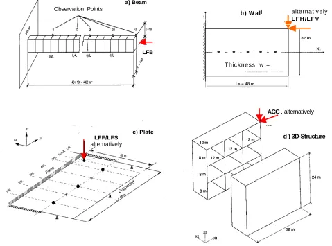
A number of characteristic, simple 1-, 2- and 3- dimensional substructures (beams, walls, plates) were selected for discretization and performances of the parametric studies. Their parameters correspond to full scale and dimensions of structures designed in reality (Fig 2a to 2d)

Observation Points

a) Beam

LFB

Fig 2. Parametric models selected to study the low passing filter effects

T h ic k nes s w =

alte rnatively L F H /L F V

b ) W all

RLF

ACC , alternatively

d ) 3D-Structure

LFF/LFS alternatively

(3)

The starting point of the discretization concept of the investigated parametric models was in each case a basic discretization variant required to capture the mode shape of the highest vibration form that could be well amplified by the impact load function (Tab 1)

The discretization of the mathematical models was then refined in several steps by reducing the element size stepwise by factor 2. However the smallest element length of the finite element discrimination was limited by the diameter of the beam parameters and thickness of the plates and walls. In order to study the wave transfer in spatial continua model concepts of axisymmetric and box shaped building structures were selected additionally (Fig 2d).

Despite the descretization ratio this models were used to study and demonstrate the, influence of various parameters (such as the character and duration of the loading function, the boundary conditions (plates) or the acting direction of the load in the grid) on the change of the structural response.

Representative Loading Functions and Element Lengths

The vibration periods Ti of the selected geometrically simple parametric model (Fig.2a) were calculated and summa-rized (Table 1). The amplification characteristics of single mass system for a triangular input function resulting to a maximum response for td/T = 1 were used to estimate the most effective duration td of the impact functions (LFB). By the same procedure the basis time for the other type of the investigated parametric models were estimated (Fig. 3).

Tab. 1 Basis time of loading functions and maximum element length for beam models

Eigenfrequencies fi (Hz) 214 Hz 643 Hz 1071 Hz 1496 Hz fn = 1919 Hz

Vibration periods Ti (s)

Selected basis time (ms)

0,005

5 0,0015 0,001 0,0007 0,0005

Td/Ti (for td = 0,005 s) 1,0 3,33 5,0 7,14 10,0

DLF = D (ST2) 1,5 1,2 1,1 1,05 1,0

Length of the beam elements (m) to grasp the modes up to f 5 (L i = 0,125 Ti c L )

2,26 0,68 0,46 0,32 0,24

The duration of the selected impact loading function were therefore chosen in all cases as equal to the period of the fundamental frequency of the investigated models . When applying the selected loading function a number of traveling shock waves, which correspond to the fundamental mode as well as to a number of higher vibration modes, are induced in the investigated parametric models..

In order to omit any adulteration of the results and achieve sufficient superimposed dynamic response every of the traveling wave must be identified (grasp) by a sufficient number of supporting points (elements)

A commonly accepted identification assumption of a traveling wave by means of 9 supporting points (wave grasp assumption) was used (Fig 1). Based on the relationship between the wave velocity (c) and the wave length (l) in the corresponding continuum as well as the assumption above mentioned, the allowable element length might be defined for the corresponding duration of the impact loading function t d .

Identifying a wave by means 9 grasp points the element length (1/8 l) is :

Li = 1/8 c t (1)

For: t d /T=1 the commonly used element Fig. 3 Representative loading functions

Length are expressed by: L i = 1/8 c Ti . The corresponding element sizes for sufficient (not mutilated) identification of the upper mode f n of a traveling shear and lengths wave may be easily obtained as:

L w (L) = 0,125 c (L) / f n (2)

and L w(L) = 0,125c (S) / f n (3)

respectively. The sizes of the elements (Tab.1)depends therefore, beside the upper frequencies of the structure fn

to be considered, also from the longitudinal velocity c (L) and shear velocity c (S) respectively of the concrete

material of the structure which are expressed by the formulas:

c (L) = E (1 - n) / r (1 + n) ( 1 – 2 n) (4)

(4)

By similar way the element lengths for other parametric models were selected (Table 2). Based on the length of elements obtained (Table 1 and 2) for the parametric models a wide variation of the element size was selected for the beam (0,1m – 0,8m) ,the plates and walls (1m x 1m to 8m x 8m) as well as for the box shaped structures.

Table 2 Element lengths derived for walls, plates an 3-D models

Type of finite element _fElement lengths (m) for upper frequency to be grasped

n-2 fn-1 fn ( 80 Hz)

Walls

Walls, axial loading (L i = 0,125 Ti c L ) _{9,0 7,7}_5,6

Walls, shear loading (L i = 0,125 Ti c S ) _{13,7 7,0}_3,4

Plates

Plates, free supported (L i = 0,125 Ti c S) _{19,5 12,3}_3,4

Plates, Fixed (L i = 0,125 Ti c S ) _{13,9 6,1}_3,4

Structures (walls an floors)

Walls (L i = 0,125 Ti c S ) _{4,8 3,9}_3,4

Floors (L i = 0,125 Ti c L ) _{7,7 6,3}_5,4

Characteristics results

In order to demonstrate and enlighten the low passing phenomena the results were shown in appropriate graphical form. Compared and demonstrated were especially the time histories of the displacements and acceleration as well as the acceleration response spectra obtained for characteristic observation points of the discretized structure.

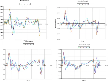
Fig. 4 Acceleration time histories in the observation points of the beam derived for discretizations 1s to 8s

Observation Piont o,4L

-6,0E+04 -4,0E+04 -2,0E+04 0,0E+00 2,0E+04 4,0E+04 6,0E+04

0,0E+00 1,0E-03 2,0E-03 3,0E-03 4,0E-03 5,0E-03 6,0E-03 7,0E-03

Time (s)

1s 2s 4s 8s

Observation Point 0,6L

-6,0E+04 -4,0E+04 -2,0E+04 0,0E+00 2,0E+04 4,0E+04 6,0E+04

0,0E+00 1,0E-03 2,0E-03 3,0E-03 4,0E-03 5,0E-03 6,0E-03 7,0E-03

Time (s) 1s 2s 4s 8s

Observation Point 0,8L

-8,0E+04 -6,0E+04 -4,0E+04 -2,0E+04 0,0E+00 2,0E+04 4,0E+04 6,0E+04 8,0E+04

0,0E+00 1,0E-03 2,0E-03 3,0E-03 4,0E-03 5,0E-03 6,0E-03 7,0E-03

Time (s)

1s 2s 4s 8s

-5,0E+04 -4,0E+04 -3,0E+04 -2,0E+04 -1,0E+04 0,0E+00 1,0E+04 2,0E+04 3,0E+04 4,0E+04 5,0E+04

0,0E+00 1,0E-03 2,0E-03 3,0E-03 4,0E-03 5,0E-03 6,0E-03 7,0E-03

Time (s)

A

ccel

er

at

ion (

m

/s2)

(5)

The comparison of results obtained for the beam model shows that in case of a moderate and fine discretisation the time histories of the displacements and accelerations are quite identical while descritization by means of rough elements shows in rather strong deviation of the results.

By first evaluating as first the time histories (Fig.4) obtained for different discretization ratio of the beam the delay of the arrival time as well as the attenuation of the amplitudes maybe recognized for all type of discretizations. Further it can be recognized that the results are identical for a fine discretization ( 1s and 2s) and it can be clearly recognized that by increasing the length of the elements to 4s and 8s the arrival time is deleted and the amplitudes are reduced.

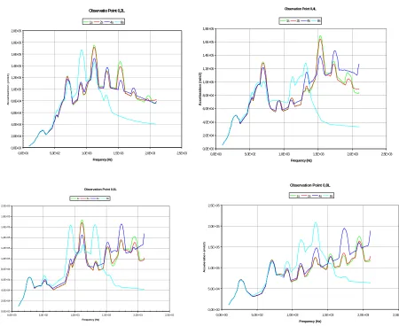
When Transferring these time histories into response spectra (Fig. 5) it can be recognized that the spectra obtained for the rougher discertization ( 4s and 8s) do not converge to the results obtained for more refined discretization.

Fig. 5 Response spectra in the observation points of the beam derived for discretizations 1s to 8s

The extended parameter studies performed for full-scale walls (Fig. b) and plates (Fig. 2c) yielded similar results with regards to the influence of the discretization used for the modeling of the structures.

In case of walls the impact loads were applied alternatively (Fig. 2b) in the axial (disc) direction as well as perpendicular to the axial (shear) direction). It could be again observed that in case of a fine discretization (1m x 1m and 2m x 2m) the dynamical response results (displacements, accelerations) are in good agreement or

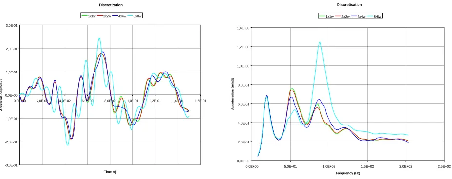
identical while of rough discretization (lager than 3x3m) a rather big deviation can bee observed (Fig 6 and 7). The dynamic response results obtained for a real scale box shaped building structure( 2d) were obtained for a

loading function corresponding to the impact of a military airplane (Phantom) [7] applied in a characteristic region of the structure. Due to the larger extension of the box shaped buildings and the associated larger wave propagation distances as well as the application of larger impulses, the dynamic response are more clearly expressed as in case of the beams, walls and plates.

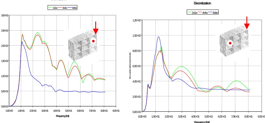
Similar as in case of the substructures, the results obtained for more refined descretization (2m x 2m and 4m x 4m) are in good agreement . The results obtained by rougher descretization (8m x 8m) do not converge especially in the frequency range above the fundamental frequency (Fig. 8 to 11).

Observatio Point 0,2L

0,0E+00 2,0E+04 4,0E+04 6,0E+04 8,0E+04 1,0E+05 1,2E+05 1,4E+05 1,6E+05 1,8E+05 2,0E+05

0,0E+00 5,0E+02 1,0E+03 1,5E+03 2,0E+03 2,5E+03

Frequency (Hz)

1s 2s 4s 8s

0,0E+00 2,0E+04 4,0E+04 6,0E+04 8,0E+04 1,0E+05 1,2E+05 1,4E+05 1,6E+05 1,8E+05

0,0E+00 5,0E+02 1,0E+03 1,5E+03 2,0E+03 2,5E+03

Frequency (Hz)

Ac

c

e

la

ra

tio

n

(m

/s

2

)

1s 2s 4s 8s

0,0E+00 2,0E+04 4,0E+04 6,0E+04 8,0E+04 1,0E+05 1,2E+05 1,4E+05 1,6E+05 1,8E+05 2,0E+05

0,0E+00 5,0E+02 1,0E+03 1,5E+03 2,0E+03 2,5E+03

Frequency (Hz)

Accel

erat

io

n

(

m

/s2)

1s 2s 4s 8s

0,0E+00 5,0E+04 1,0E+05 1,5E+05 2,0E+05 2,5E+05

0,0E+00 5,0E+02 1,0E+03 1,5E+03 2,0E+03 2,5E+03

Frequency (Hz)

(6)

Fig. 6 Time histories and response spectra in the center of the shear wall , loading function LFH

Fig. 7 Time histories and response spectra in the center of the fixed plate, loading function LFF

Fig. 8 Response spectra (X1) in characteristic Region of the structure due to horizontal loading Discretization

-3,0E-01 -2,0E-01 -1,0E-01 0,0E+00 1,0E-01 2,0E-01 3,0E-01

0,0E+00 2,0E-02 4,0E-02 6,0E-02 8,0E-02 1,0E-01 1,2E-01 1,4E-01 1,6E-01

Time (s)

1x1w 2x2w 4x4w 8x8w

Discretisation

0,0E+00 2,0E-01 4,0E-01 6,0E-01 8,0E-01 1,0E+00 1,2E+00 1,4E+00

0,0E+00 5,0E+01 1,0E+02 1,5E+02 2,0E+02 2,5E+02

Frequency (Hz)

1x1w 2x2w 4x4w 8x8w

Discretization

0,0E+00 2,0E-01 4,0E-01 6,0E-01 8,0E-01 1,0E+00 1,2E+00 1,4E+00 1,6E+00

0,0E+00 2,0E+01 4,0E+01 6,0E+01 8,0E+01 1,0E+02 1,2E+02

Frequency (Hz)

1x1 2x2 4x4 8x8 Discretization

0,0E+00 2,0E-01 4,0E-01 6,0E-01 8,0E-01 1,0E+00 1,2E+00 1,4E+00 1,6E+00

0,0E+00 2,0E+01 4,0E+01 6,0E+01 8,0E+01 1,0E+02 1,2E+02

Frequency (Hz)

1x1 2x2 4x4 8x8

Discretization

0,0E+00 1,0E+01 2,0E+01 3,0E+01 4,0E+01 5,0E+01 6,0E+01 7,0E+01 8,0E+01 9,0E+01

0,0E+00 1,0E+01 2,0E+01 3,0E+01 4,0E+01 5,0E+01 6,0E+01 7,0E+01 8,0E+01 9,0E+01 Frequency (Hz)

Accelaration (m/s2)

2x2w 4x4w 8x8w Discretization

0,0E+00 2,0E+01 4,0E+01 6,0E+01 8,0E+01 1,0E+02 1,2E+02

0,0E+00 1,0E+01 2,0E+01 3,0E+01 4,0E+01 5,0E+01 6,0E+01 7,0E+01 8,0E+01 9,0E+01

Frequency (Hz)

Accel

erat

io

n

(m/

s2)

(7)

Fig 9 Response spectra (X1) in characteristic Region of the structure due to horizontal loading

Fig. 10 Response spectra (X3) in characteristic Region of the structure due to vertical loading

Fig 11 Response spectra (X3) in characteristic Region of the structure due to vertical loading

Characteristic Region

0,0E+00 1,0E+01 2,0E+01 3,0E+01 4,0E+01 5,0E+01 6,0E+01 7,0E+01 8,0E+01 9,0E+01

Frequency (Hz)

2x2w 4x4w 8x8w

Discretization

0,0E+00 5,0E+01 1,0E+02 1,5E+02 2,0E+02 2,5E+02 3,0E+02

2x2w 4x4w 8x8w

Characteristic Region

0,0E+00 1,0E+01 2,0E+01 3,0E+01 4,0E+01 5,0E+01 6,0E+01 7,0E+01

0,0E+00 1,0E+01 2,0E+01 3,0E+01 4,0E+01 5,0E+01 6,0E+01 7,0E+01 8,0E+01 9,0E+01

Frequency (Hz)

2x2w 4x4w 8x8w

Discretization

0,0E+00 1,0E+01 2,0E+01 3,0E+01 4,0E+01 5,0E+01 6,0E+01 7,0E+01 8,0E+01 9,0E+01 1,0E+02

2x2w 4x4w 8x8w

Discretization

0,0E+00 2,0E+01 4,0E+01 6,0E+01 8,0E+01 1,0E+02 1,2E+02

0,0E+00 1,0E+01 2,0E+01 3,0E+01 4,0E+01 5,0E+01 6,0E+01 7,0E+01 8,0E+01 9,0E+01

Frequency (Hz)

2x2w 4x4w 8x8w

Discretization

0,0E+00 1,0E+01 2,0E+01 3,0E+01 4,0E+01 5,0E+01 6,0E+01 7,0E+01 8,0E+01

0,0E+00 1,0E+01 2,0E+01 3,0E+01 4,0E+01 5,0E+01 6,0E+01 7,0E+01 8,0E+01 9,0E+01

Frequency (Hz)

(8)

Verification of Discretization Criteria

By comparing and evaluating the extensive results obtained it is possible to identify unambiguous the passing element length limits (low-pass filter element lengths) of the FE models, which are characterized by the fact that the structural responses (time histories, spectra) determined on such a basis are still in a good agreement and display satisfactory convergence with results obtained with a finer element mesh.

The element lengths defined by the common wave grasp assumption ( 9 supporting points) are to large ,so in case of short duration loading, one part of the propagating waves is filtered. A correction of the element length is urgently required. The starting point of the correction procedures are the convergence – element length obtained by means of the parametric studies performed for the corresponding substructures (beam, walls, plates) as well as 3D-buildings structures and the corresponding correction factor obtained. The corresponding correction factor (k) are expressed by the relation of the derived convergence element length (Lk) to the length obtained by the

common wave grasp assumption (Lw). The correction factors are related (Table 2) to the highest mode (fn = 80

Hz) to be considered in practical design of safety relevant systems in case of aircraft crash loading.

Based on the values of the convergence correction factor k obtained within the studies as well as the length obtained by the common wave grasp assumption (Tables 1 and 2) the following empirical formulas were derived for the definition of the element length discretization of the corresponding structure.

- Beams, Columns Lk (B) £ c L / 12 fn

- Walls , Discs Lk (W) £ c L / 22 fn

- Plattes, Floors Lk (P) £ c L,S / 16 fn

- Box Shaped Structures Lk (S) £ c L,S / 16 fn

The empirical formulas can be used to specify the suitable mesh for discretizing the respective substructures i.e. the largest allowable element size which allows the derivation of results, which are within the range of reliability. The dispersion effects were obsererved as well but not evaluated within these studies. To clarify this phenomena of finite element models additional investigations seems to be required .

Summary

It could be pointed out that in case of impact loading the response results obtained by means of common state of the art procedures do not provide suitable for practical use results.

Even a commonly used wave grasp assumption is strictly applied ,it is not possible to specify an appropriate size of a finite element (or the mesh of a FE model ) to achieve reliable results for given impact loads.

The element sizes determined on this basis prove be too large. However, appropriate FE model discretizations for handling impact problems can be specified and reliable results determined on the basis of the convergence element size Lk .

Empirical relationships based on these parametric studies are proposed for future applications by which the allowable element size Lk of the discretizations of a finite element model can be determined on the basis of the

frequency range fn to be considered in case of the investigated dynamic problem as well as on the basis of

physical wave velocities that corresponds to the material of the structure.

References

[1] Kolsky, H.. Stress Waves in Elastic Solids, Springer Verlag Berlin, 1964

[2] Constantino, C.J. Finite Element Approach to Stress Wave Problems Journal of the Engineering Mechanics

Division, American Society of Civil Engineers, April 1967

[3] Shipley, SA, Leistner, H.G., Jones R.F. Elastic Wave-Propagation – A comparison between Finite Element

Predictions And Exact Solutions, Dynamic of Earth Material, University of Stanford, (1981)

[4] Bielor E. , Freiman M., Krutzik N.J. Accuracy of Dynamic Calculations Using Shell Models Under Impulse

Loading , Nuclear Engineering and design 117/ 1987

[5] Freund, H. U., Krutzik, N. J., Müller, K. Local Response of Concrete Structures due to Explosive Loading,

SMiRT 10th Conference, Los Angeles 1989

[6] Krutzik, N.J. Applicability of Finite Element Models for Simulation of Shock Transfer Processes in Nuclear Power Plants due to Impact Loading, University of Karlsruhe, February 2002, S Dissertation