Transactions of the 17th International Conference on Structural Mechanics in Reactor Technology (SMiRT 17)
Prague, Czech Republic, August 17 –22, 2003
Paper # K03-4
Artificial Ground Motion with Non-Stationarity Generated using the Wavelet Analysis
Fumio Sasaki1), Toshiro Maeda2), Yoshifumi Yamamoto1)
1)
Kajima Corporation, Tokyo, Japan
2)
Waseda University, Tokyo, Japan
ABSTRACT
We have proposed a new method of constructing artificial ground motion with non-stationarity, which is necessary to evaluate the frequency selective resonance of non-linear structures. The wavelet transform with the Sinc wavelets is used to decompose signal into band-limited frequency contents with temporal shifts, thus expressing the non-stationarity. Squared wavelet coefficients are modeled by the normal distribution along time axis, with the acceleration power, the temporal centroid, and the temporal variance evaluated by magnitude and epicentral distance. Artificial ground motion is generated by the inverse wavelet transform to show the non-stationarity inferred from wave propagation and statistically anticipated attenuation relations.
KEY WORDS: Wavelet Analysis, Sinc Wavelets, Group Delay Time, Artificial Ground Motion, Non-stationarity,
Regression Analysis.
INTRODUCTION
Since non-linear structures have a tendency of selective resonance with varied frequencies according to their degrading nature, non-stationarity with frequency contents may play an important role in evaluating response and damage of structures. An artificial ground motion is usually constructed by conforming time series to the defined response spectra with random phase and envelope functions, thus the non-stationarity in amplitude can be modeled but the non-stationarity in frequency contents can not. Other studies have used group delay time to model Fourier phase and shown non-stationarity in frequency contents, however, contribution from Fourier amplitude to the non-stationarity has been fully neglected.
In this study, we have used wavelet transform, which can express time signal by combination of time shifted similar wavelets with different time spans. We can control temporal variation of frequency-banded signals by properly placing wavelet coefficients along time axis and exhibit non-stationarity without help of group delay time. The placement of wavelet coefficients is statistically determined by its centroid and variance equivalent to time signal counterparts; the amplitude by energy with wavelet coefficients equivalence as well. These coefficients values are determined by regression analysis with several earthquake ground motion data.
DIFINITION OF SINC WAVELETS
The Sinc function defined in Eq.1 and Eq.2 for discrete case in eligible for scaling function in the wavelet analysis.
t t t
Sinc()=sinπ /π ,Sˆinc(ω)=1(−π ≤ω<π),0(otherwise), (1)
) otherwise (
0 ), ( 2 / 1 ), ( 1 ) (
ˆincω = ω <π ω =π
S (2)
where ^ expresses Fourier domain.
The mother wavelet can be constructed from the Sinc function in the wavelet analysis. The mother wavelet can be constructed from the Sinc function via the multi-resolution analysis shown in Eq.3 and Eq.4 [1].
) 2 / 1 ( 2
) 2 / 1 ( 2 sin 2 ) 2 / 1 (
) 2 / 1 ( sin ) (
− − −
− − =
t t t
t t
π π π
π
where Ψˆ(ω)=1(π <ω <2π),1/ 2(ω =π,2π),0(otherwise) (4)
The Sinc wavelets are defined as the family {ψj,l| j,l∈Z} expressed by Eq.5, where level j implied a scale factor corresponding to frequency band, shift l corresponds to time shift.
) 2 ( 2 ) ( 2
, t t l
j j l
j = ψ −
ψ , (5)
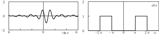
In time domain the mother wavelet is very smooth and infinitely differentiable, in frequency domain it has compact supports as shown in Fig.1.
abs 0 1 2 ω -π π
-2π 0 2π
-2 0 2
tim e
6 0 6
Fig. 1 The shape of mother wavelet in time and frequency domain
The Sinc Wavelets of level j have support range corresponding to frequency band of [2 1/ ,2 / ]
T
T j
j−
, where T
is duration time. The Sinc wavelets have favorable characteristics of avoiding serious overlap between frequency bands, just two points on each frequency band boundaries of each level. The orthonormal wavelet transform and its inverse wavelet transform are defined by Eq.6 [1], [2], where αj,l is call wavelet coefficients and expresses complex
conjugate. dt t t f j j
∫
∞ ∞ − = () , (),l ψ l
α , () () , () 0 1 2 0 , 0 t t f t f j j j j j j l l l ψ α
∑ ∑
∑
∞ = − = ∞ = == , (6)
NON-STATIONARY PARAMETERS EXPRESSED BY WAVELET COEFFICIENTS
Definitions of Non-Stationary Parameters
Izumi and Katsukura [3] and Sato et al. [4] defined the expression of total energy of complex envelope in time domain, temporal centroid and temporal variance by
∫
∫
= = ∞ ∞ − N d A dt t fE ω ω ω
π 0 2 2 ) ( 2 ) ( ) )
, = =
∫
NA tgr dE t tgr ω ω ω ω π µ 0 2
0 ( ) ( )
2
) , 2 2 2
dA tgr
t σ σ
σ = + (7)
{
}
∫
− = N d tgr A E tgr tgr ω ω µ ω ω π σ 0 2 2 2 ) ( ) ( 2 ) ,∫
= N d d dA E dA ω ω ω ω π σ 0 22 2 ( )
)
, (8)
where ωNis Nyquist frequency, and Fourier transform of f(t) and f(t)
)
, and group delay time tgr(ω) are defined by )} ( exp{ ) ( ) exp( ) ( )} ( exp{ ) ( ) exp( ) ( ω ϕ ω ω ω ϕ ω ω i F dt t i t f i A dt t i t f − = − − = −
∫
∫
∞ ∞ − ∞ ∞ − )) , where <
≥ = 0 0 0 ) ( 2 ) ( ω ω ω ω A
F) (9)
ω ω ϕ ω d d
tgr( )= ( ) (10)
In above equations, temporal centroid and temporal variance of complex envelope f)(t) are equal to those of time signal f(t), and energy of complex envelope is twice as that of time signal.
Izumi and Katsukura [3] showed that in the analysis for some of Minyagi-ken-Oki earthquake (1978) records,
2
tgr
for some of Izu-Oshima-Kinkai earthquake records, 2
tgr
σ was 4 times greater than 2 dA
σ . Despite the fact that these studies have pointed out the importance of the ratio of σtgr2 and
2 dA
σ , farther analysis have not appeared yet. This may be because tgr(ω) fits the usual approach very well, and the group velocity of surface waves can be explained by
) (ω
tgr adequately.
In this study, acceleration power Ej, temporal centroid µj, temporal variance
2
j
σ are defined by Eq.11, where )
(t
fj is band limited wave obtained by restraining certain level j in Eq.6.
∫
−∞∞= ω ω ω
π f f d
Ej ˆj( )ˆj( )
2 1 , =
∫
−∞∞ ω ω ω ω πµ f d
d f d E i j j j
j ˆ ( )
) ( ˆ
2 ,
2
2 ˆ ( ) ˆ ( )
2 1 j j j j j d d f d d f d
E ω ω µ
ω ω ω π σ =
∫
∞ − ∞− (11)
Eq.11 can be written as Eq.13 with wavelet coefficients by using orthonormal characteristics of Sinc wavelets shown in Eq.12.
l k l j k j l j k
j, t , tdt ˆ , ( )ˆ ,( )d ,
2 1 ) ( ) ( ψ ωψ ω ω δ π ψ ψ =
∫
=∫
−∞∞ ∞ ∞− (12)
∑
−=
=2 1
0 2 , j k k j j
E α , j
l l j j j j E l j / 2 1 2 1 2 0 2 , 1
∑
− = + + = αµ , 2
1 2 0 2 , 2 1 2 / 2 1
2 j j
l l j j j j E l j
µ
α
σ
− + =∑
−= + (13)
By Eq.13, we can directly compute acceleration power, temporal centroid and temporal variance in each level j, from wavelet coefficients. In above equations, f(t) is assumed as a periodic function of 1 second so that the modification should needed for periodic function for T second. Ej→Ej⋅T , µj→µj⋅T ,
2 2
2 T
j j →σ ⋅
σ .
General Characteristics of Non-Stationary Parameters
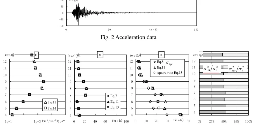
The non-stationary parameters defined in Eq.13 are shown in Table1 and Fig.2 for Kagoshima-ken-Hokuseibu earthquake, Gamo station (NS-comp) to be parted the dataset of the next section. The duration of data is 163.84 seconds, and 0 data of 163.84 seconds are inserted before its origin to avoid link effect in the computation.
-150 -75 0 75 150
0 50 tim e(s)100 150
acc(gal)
Fig. 2 Acceleration data
4 5 6 7 8 9 10 11 12 13
0 20 40 60 80 100 level(j) Eq.7 Eq.11 Eq.13 tim e(s) μ 4 5 6 7 8 9 10 11 12 13level(j) E q.11 E q.14
(cm2/sec2)
1e-1 1e+3 1e+7
E 4 5 6 7 8 9 10 11 12 13
0 10 20 30 40 50 level(j)
Eq.8
Eq.11 square root Eq.13
tim e(s) σ
0% 25% 50% 75% 100% 4 5 6 7 8 9 10 11 12 13level(j)
Fig. 3 Non-stationary parameter (from left : Ej
~
, µj, σj, ratio of
2 2
t dA σ
σ and σtgr2 σt2)
2 2
t dA σ
σ 2 2
t tgr σ
σ
tgr
Table 1 Non-stationary parameters of the Kagoshima-ken-Hokuseibu earthquake
j µj σj E~ j Frequency band (Hz)
4 13.29 42.19 2.37E-1 0.02~0.05
5 14.73 21.94 1.08E+0 0.05~0.10 6 10.82 20.93 9.09E+0 0.10~0.20
7 27.56 24.09 8.40E+1 0.20~0.39 8 28.84 15.51 4.52E+3 0.39~0.78 9 23.86 9.71 7.89E+3 0.78~1.56 10 16.24 5.10 2.63E+3 1.56~3.13
11 13.90 3.51 5.56E+2 3.13~6.25 12 12.50 3.02 3.39E+2 6.25~12.5 13 12.60 3.43 1.75E+2 12.5~25.0
Acceleration power Ej computed by wavelet coefficients (Eq.13) completely equals to the one by time history
(Eq11) as shown in Fig.3. Ej has a predominance from 0.4 to 3 Hz. In Fig.3, acceleration power normalized by the
support frequency range is shown in Fig.3 to make comparison between levels easier.
∑
∑
−= − −
=
− =
−
= 2 1
0 2
, 1 1
2
0 2
, 1
~
2 2
2
j j
k k j j
k k j j
j j
T T
E α α (14)
In Fig.3, temporal centroid of acceleration data is almost the same value as temporal centroid of wavelet coefficients. Temporal standard deviation computed by acceleration data almost equals to temporal standard deviation by wavelet coefficients excluding small levels. And standard deviation of group delay time σtgr is smaller than standard
deviation of wavelet coefficients because it does not include σdA. Fig.3 shows a predominance of acceleration power in
0.8-3 Hz. Temporal centroid appears later and temporal standard deviation becomes larger as frequency becomes over 0.4Hz. These figures show non-stationary parameters computed by wavelet coefficients is equivalent to that computed by time history.
In addition, in Fig.3 we indicate average value of 2 2 t dA σ
σ and 2 2
t tgr σ
σ for all NS acceleration data of Kagoshima-ken-Hokuseibu earthquake to discuss the influence of σdA. This figure shows that
2 dA
σ has as almost the same influence as 2
tgr
σ , and indicate the necessity of evaluating 2 dA
σ .
ARTIFICIAL GROUND MOTION GENERATION
In this section, we propose the way to generate wavelet coefficients from µj,
2
j
σ , E~j . First, we model µj,
2
j
σ ,
~
j
E by multi-regression analysis with magnitude and epicentral distance, then we propose the method to generate the
artificial ground motion from magnitude and epicentral distance. In addition, data used in this section is transformed as well as in former section to avoid link effect.
Wavelet Coefficients Generation
Although Iyama and Kuwamura [5] assume that the envelope of wavelet coefficients is triangle distribution from the relation between acceleration data of input energy and accumulated squared wavelet coefficients, in this study we assume that envelope of wavelet coefficients is normal distribution [µj,σ2j] It is necessary to discuss more in the empirical point for the shape of envelope. So we give the squared wavelet coefficients in each level having the power that is as the same as Ej, and we determine sign of wavelet coefficients from uniform random number. Wavelet
coefficients αj,l represent non-stationary parameter of the position l T j j+1/2 )⋅
2 /
-150 -75 0 75 150
0 50 tim e(s)100 150 acc(gal)
(analysis)
0 50 100 150
0 5 10 15freq.(H z)20 25 (gal・s)
(analysis) -150
-75 0 75 150
0 50 tim e(s)100 150 acc(gal)
(observation)
0 50 100 150
0 5 10 15freq.(H z)20 25 (gal・s)
(observation)
1.0223E-2 4.0876E+1
0 tim e(s) 80
0.25H z
8.0H z
2.1367E-2 3.3588E+1 0.25H z
8.0H z
0 tim e(s) 80 (observation) (analysis)
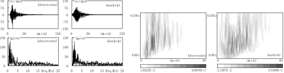
Fig. 7 The observation and analysis (left : Acceleration data and Fourier amplitude, right : Wavelet coefficients)
To demonstrate the effectiveness of this method, we compare the observation record with the artificial ground motion computed by µj,
2
j
σ and E~j (Table 1) of the KGS008(K-NET, Δ=31km, NS-component) about Kagoshima-ken-Hokuseibu earthquake(M=6.3). Fig.7 shows acceleration data, Fourier amplitude and absolute value of wavelet coefficients by continuous wavelet transform in time-frequency domain. Origin of this data is defined as the earthquake occurrence time. Continuous wavelet transform is applied for 80 seconds of data. In this example, observation record is almost reproduced including stationarity. Therefore, it is possible to generate the artificial ground motion with non-stationarity by µj,
2
j
σ and E~j properly modeled about magnitude and epicentral distance.
Multi-Regression Analysis
We use multi-regression analysis with Eq.15 (like Sato et al. [6]) for evaluatingµj, σj and
~
j
E computed by
wavelet coefficients. Table 2 shows the data used in this study, whose maximum acceleration is over 30 gal. Fig.8 shows the relations of magnitude and epicentral distance in these data. We use multi-regression analysis forµj,
2
j
σ and E~j
by magnitude and epicentral distance, which are computed from each data in Table 2.
j j j j
µ
µ γ
β µ
α
µ = ⋅ M⋅∆
10 , j j
j j
σ
σ γ
β σ
α
σ = ⋅ M⋅∆
10 , Ej Ej
Ej j
E~ =α ⋅10β M⋅∆γ (15)
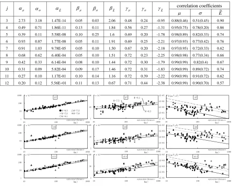
Table 3 shows regression coefficients αj, βj, γj and correlation coefficients for each level. Correlation
coefficients for µj and σj becomes larger as levels become higher, correlation coefficients for
~
j
E is indifferent with levels. For reference, we use multi-regression analysis about average and variance of tgr(ω) like Sato et al [6]. Table 3 shows that correlation coefficients for average of tgr(ω) in parentheses is as almost the same value as correlation coefficient for µj, but correlation coefficient for variance of tgr(ω) is a little smaller than correlation coefficient for
j
σ using wavelet coefficients. So temporal variance along time axis by wavelet coefficients is more stable than by )
(ω
tgr in this study.
Fig.9 shows comparison of regression curve and µj, σj and
~
j
E . In this figure, µj appears later as epicentral
distance becomes longer because wave arrival time becomes later. And
~
j
E becomes smaller because of geometric damping. In addition, σj becomes longer by the scattering and the dispersion of the earthquake ground motion and σj
as well as E~j becomes larger as magnitude becomes larger.
Table 2 The earthquake data used in this study (right: Fig.8 The relationship of magnitude and epicentral distance)
date name magnitude number of data seismograph
07/12/1993 Hokkaido-nansei-oki 7.8 2 JMA87
10/07/1994 Hokkaido-Toho-Oki 8.1 18 JMA87
12/28/1994 Sanriku-Haruka-Oki 7.5 14 JMA87
01/17/1995 Hyogo-ken-Nanbu 7.2 16 JMA87
03/26/1997 Kagoshima-ken-Hokuseibu 6.3 69 K-NET95
1 10 100 1000
Table 3 The result of multi-regression analysis (In parentheses, the result about group delay time)
correlation coefficients
j αµ ασ αE~ βµ βσ
E~
β γµ γσ γE~
µ σ E~
3 2.73 3.18 1.47E-14 0.05 0.03 2.06 0.48 0.24 -0.95 0.88(0.46) 0.51(0.45) 0.90
4 0.49 0.71 1.86E-11 0.13 0.11 1.84 0.56 0.27 -1.31 0.95(0.75) 0.78(0.20) 0.86
5 0.39 0.11 5.58E-08 0.10 0.25 1.6 0.69 0.20 -1.78 0.98(0.89) 0.82(0.33) 0.74
6 0.93 0.87 1.77E-08 0.05 0.11 1.91 0.69 0.25 -2.21 0.97(0.93) 0.77(0.42) 0.76
7 0.91 1.03 9.78E-05 0.05 0.10 1.50 0.67 0.20 -2.18 0.97(0.95) 0.72(0.33) 0.62
8 0.68 0.62 6.40E-04 0.05 0.10 1.51 0.72 0.23 -2.25 0.98(0.98) 0.77(0.34) 0.66
9 0.42 0.33 6.14E-04 0.08 0.10 1.44 0.72 0.30 -1.79 0.99(0.99) 0.82(0.4) 0.67
10 0.31 0.09 5.82E-04 0.09 0.17 1.46 0.72 0.31 -1.83 0.99(0.99) 0.89(0.72) 0.74
11 0.27 0.10 1.17E-01 0.10 0.14 1.16 0.72 0.39 -2.22 0.99(0.99) 0.91(0.72) 0.62
12 0.20 0.12 5.56E+01 0.11 0.13 0.67 0.71 0.44 -2.38 0.99(0.99) 0.90(0.70) 0.57
j=9
1.E-01 1.E+01 1.E+03 1.E+05 1.E+07
10 100 epicentral distance(km ) 1000
E(cm2/s2) j=9
1 10 100
10 100 epicentral distance(km ) 1000 σ(s)
j=9
1 10 100 1000
10 100 epicentral distance(km ) 1000 μ(s)
j=11
1.E-01 1.E+01 1.E+03 1.E+05 1.E+07
10 100 epicentral distance(km ) 1000
E(cm2/s2) j=11
1 10 100
10 100 epicentral distance(km ) 1000 σ(s)
j=11
1 10 100 1000
10 100 epicentral distance(km ) 1000 μ(s)
j=7
1.E-01 1.E+01 1.E+03 1.E+05 1.E+07
10 100 epicentral distance(km ) 1000
E(cm2/s2) j=7
1 10 100
10 100 epicentral distance(km ) 1000 σ(s)
M =6.3 M =8.1 M =7.5
j=7
1 10 100 1000
10 100 epicentral distance(km ) 1000 μ(s)
●M =6.3 △M =7.2 ×M =7.5 *M =7.8 ◇M =8.1
Fig. 9 The result of multi-regression analysis in the level from 7 to 12
Example of Artificial Ground Motion
-150 0 150
0 40 tim e(s) 80
acc(gal)
j=11
-40 0 40
0 40 tim e(s)80
acc(gal)
j=11
-10 0 10
0 40 tim e(s)80
acc(gal)
j=11 -150
0 150
0 40 tim e(s) 80
acc(gal)
j=9
-40 0 40
0 40 tim e(s)80
acc(gal)
j=9
-10 0 10
0 40 tim e(s)80
acc(gal)
j=9 -150
0 150
0 40 tim e(s) 80
acc(gal)
epicentral distance=10km j=8
-40 0 40
0 40 tim e(s)80
acc(gal)
epicentral distance=30km j=8
-10 0 10
0 40 tim e(s)80
acc(gal)
epicentral distance=100km j=8
-150 0 150
0 40 tim e(s) 80
acc(gal)
j=10
-40 0 40
0 40 tim e(s)80
acc(gal)
j=10
-10 0 10
0 40 tim e(s)80
acc(gal)
j=10
-150 0 150
0 40 tim e(s) 80
acc(gal)
j=12
-40 0 40
0 40 tim e(s)80
acc(gal)
j=12
-10 0 10
0 40 tim e(s)80
acc(gal)
j=12
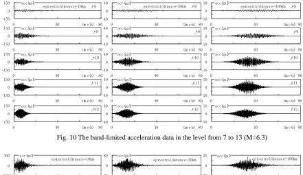
Fig. 10 The band-limited acceleration data in the level from 7 to 13 (M=6.3)
-300 0 300
0 40 tim e(s)80
acc(gal)
epicentral distance=10km
-80 0 80
0 40 tim e(s)80
acc(gal)
epicentral distance=30km
-25 0 25
0 40 tim e(s)80
acc(gal)
epicentral distance=100km
Fig. 11 The examples of the artificial ground motion (M=6.3)
Fig.11 shows acceleration data of the artificial ground motion consist of all frequency bands. In three figures, temporal centroid appears later and increase of duration becomes remarkable, as epicentral distance becomes longer. In the latter half of the wave, the component of long period is superior, so non-stationarity of frequency is realized. In this study, decrease of amplitude by the damping of energy is a little smaller than the attenuation of Fukushima and Tanaka [7]. In Fukushima and Tanaka [7], if epicentral distance is 10, 30 and 100km, maximum acceleration is 297, 126 and 26 gal respectively. Thus this study consists with the past study.
CONCLUSION
We proposed the method to generate the artificial ground motion with non-stationary by directly modeling wavelet coefficients from multi-regression analysis. With this method, it is possible to express the duration in each frequency band including the influence of Fourier amplitude to variance along time axis, which has not been considered.
We used Sinc wavelets, whose overlap between frequency bands is minimum. Sinc wavelets make the independency of the parameters of each frequency band high, and the correspondence between level and frequency band possible. And we proposed the formulation to compute acceleration energy and non-stationary parameters from wavelet coefficients directly. We confirmed that acceleration energy and non-stationary parameters from wavelet coefficients were comparable with parameters computed by acceleration data. However, it will be necessary to discuss more about the envelope in the case with large difference between envelope of observation and normal distribution because we assumed that the envelope of absolute squared wavelet coefficients was normal distribution.
In the future we will examine the envelope of squared wavelet coefficients to model the earthquake ground motion with multi-source, and we will construct acceleration power and non-stationary parameters modeled in each frequency band, including region, subsurface soil, focal mechanism, depth, and hypocentral distance.
ACKNOWLEDGEMENTS
REFERENCES
1. Daubechies, I., Ten Lectures on Wavelet, CBMS-NSF Regional Conference Series in Applied Mathmatics, CBMS-61, SIAM, 1992
2. Sasaki, F. and Yamada, M., : Biorthogonal Wavelets Adapted to Integral Operators and Their Applications, JJIAM, Vol.14, No. 2, pp.257-277, 1997.
3. Izumi, M. and Katsukura, H., A Fundamental Study on Extraction of Phase-Information in Earthquake Motions (in Japanese), J. Struct. Constr. Eng., AIJ, No.327, 20-27, May, 1983
4. Sato, T., Sato, T., Uetake, T. and Sugawara, Y., A Fundamental Study for Envelope Characteristics of Long Period Strong Motions By Using Group Delay Time (in Japanese), J. Struct. Constr. Eng., AIJ, No.480, 57-65, Feb., 1996 5. Iyama, J. and Kuwamura, H., Application of Wavelet Inverse Transform for Numerically Simulated Earthquake
Motions (in Japanese), J. Struct. Constr. Eng., AIJ, No.512, 47-54, Dec., 1997
6. Sato, T., Murono, Y. and Nishimura, A., Empirical Modeling of Phase Spectrum of Earthquake Moion (in Japanese), Journals of the Japan Society of Civil Engineers, JSCE, No.640/I-50, pp.119-130, Jan., 2000. 7. Fukushima, Y. and Tanaka, T., A new attenuation relation for peak horizontal acceleration of strong earthquake