ABSTRACT
STOUT, MALCOLM RUSSELL JR. Cooling Tower Fan Control for Energy Efficiency. (Under the direction of Dr. James W. Leach)
This thesis evaluates the economics of alternative cooling tower capacity control
methods. Annual fan electrical energy requirements are calculated for towers with
single-speed, two-single-speed, and variable-speed fans. Fan energy requirements are determined for
counter-flow and cross-flow towers designed for low initial cost and for energy efficiency.
Effectiveness-NTU equations are solved to predict cooling tower performance at various fan
speeds. Natural convection, which determines the cooling capacity when the fan is off, is
accounted for using a mean enthalpy difference. Ambient conditions are simulated using
typical meteorological year data for five locations. The results show that potential savings
are not strongly dependent on the approach temperature, but do increase with increasing
range in colder climates. The potential for saving is greatest for cooling towers designed for
low initial cost, and is generally higher in locations where the wet-bulb temperature remains
relatively constant throughout the year. Two-speed fans that can operate at half speed are
generally more suitable for low-cost cooling towers. Two-speed fans that can operate at
two-third speed are better for towers designed for energy efficiency and are generally better when
Biography
Malcolm Russell Stout Jr. was born in Southern Pines, North Carolina on September
7, 1959. In 1963, he moved with his parents to Lillington, North Carolina. He attended
school in Lillington and graduated from Lillington High School in 1977.
He earned a Bachelor of Science Degree in Geology from Campbell University in
May 1982. He worked as a chemist for a mining company for 2 years and as an engineering
technician for a geotechnical engineering company for 4 years before returning to North
Carolina State University in 1989. He earned a Bachelor of Science Degree in Mechanical
Engineering in 1991. He worked as a plant engineer at Harris Nuclear Plant for 6 years and
became a licensed Professional Engineer in North Carolina in 1996. In 1998, he returned to
North Carolina State University to begin studies toward fulfillment of a Master of Science
Degree in Mechanical Engineering. Graduate work focused on the thermal sciences
including coursework in heat transfer and fluid mechanics. From May 1998 until August
2000, he worked at the Industrial Assessment Center as a research assistant. In October
2000, he began work at the NC Department of Correction as a Facility Mechanical Engineer
and continued working there following completion of the requirements for MSME in May
Acknowledgements
This thesis would not have been possible without the support of my wife, Rose, and
the inspiration of my new baby girls, Hannah and Emma.
I would like to thank Dr. James Leach and Dr. Herb Eckerlin for their practical-
minded approach to engineering and the opportunity to broaden my engineering experience
TABLE OF CONTENTS
LIST OF TABLES v
LIST OF FIGURES vi
LIST OF SYMBOLS vii
1.0 OBJECTIVE 1
2.0 INTRODUCTION 1
2.1 Project Background 1
2.2 Cooling Towers in Industry 2
3.0 COOLING TOWER PERFORMANCE MODEL 4
3.1 Cooling Tower Capacity 4
3.2 Forced Draft - Effectiveness-NTU 5 3.3 Natural Draft – Mean Enthalpy Difference 8
3.4 Predicted Performance 9
4.0 RESULTS AND DISCUSSION 14
4.1 Capacity Control Options and the Effect of Natural Convection 14
4.2 Constant Load Applications 20
4.3 Similar Applications in Various Climates 25
4.4 Ideal Second Speed 37
4.5 Comparison of Equipment Cost and Estimated Savings 39
5.0 CONCLUSIONS 39
6.0 REFERENCES 40
7.0 APPENDICES 42
7.1 Fortran Model for Counter-flow Cooling Tower 43 – Single Operating Condition
LIST OF TABLES
TABLE 4.1 – Fan Energy Savings for Constant Load Raleigh, NC 24
TABLE 4.2 – Fan Energy Savings for Counterflow Towers Raleigh NC 24
LIST OF FIGURES
Figure 3.1 Cooling Tower Performance Calculations 12
Figure 3.2 Cooling Tower Performance Predictions 13
Figure 4.1 Capacity Control with No Free Convection 16
Figure 4.2 The Effect of Free Convection 17
Figure 4.3 Fan-Speed Options, Range = 10 °F 18
Figure 4.4 Fan-Speed Options, Range = 40 °F 19
Figure 4.5 Annual Fan Energy Consumption, Approach = 7 °F 23 Raleigh, NC
Figure 4.6 Single-Speed Fan Energy Usage for Various Locations 30
Figure 4.7 Fan Energy Savings, Range =10 °F, Approach =7 °F, 31 c=3, n=0.4, Co=0.134
Figure 4.8 Fan Energy Savings, Range =40 °F, Approach =7 °F, 32 c=3, n=0.4, Co=0.134
Figure 4.9 Wet-bulb Distribution for Typical Year in Houston and 33 Columbus
Figure 4.10 Variable Speed Drive Savings as Percentage of Single- 34 Speed Consumption for Various Locations and Operating
Conditions
Figure 4.11 Fan Energy Savings, Range =10 °F, Approach =7 °F, 35 c=1.33, n=0.4, Co=0.056
Figure 4.12 Fan Energy Savings, Range =40 °F, Approach =7 °F, 36 c=1.33, n=0.4, Co=0.056
LIST OF SYMBOLS
εa dimensionless variable defined by (hao - hai) / (hswi – hai)
εw dimensionless variable defined by (Twi - Two) / (Twi – Tawb)
m* dimensionless variable defined by (ma Cs) / (mw Cpw )
NTU dimensionless variable defined by (hc A) / (ma Cs )
Cs effective specific heat of moist air defined by (hswi – hswo) / (Twi – Two)
ma mass flow rate of air
mw mass flow rate of water
Cpw specific heat of water
hc heat transfer coefficient
A heat transfer surface area
hao enthalpy of air out
hai enthalpy of air in
hswi enthalpy of saturated air at the entering water temperature
hswo enthalpy of saturated air at the leaving water temperature
Twi temperature of water in
Two temperature of water out
Tawb wet-bulb temperature of ambient air
mwi mass flow rate of water in
mwo mass flow rate of water out
Wo humidity ratio of air in
cfm0 volumetric airflow due to natural convection
cfm volumetric airflow capacity of cooling tower
∆h mean enthalpy difference with fan off
∆hn mean enthalpy difference at nominal conditions with fan running
∆ho enthalpy difference at top of tower defined by hswi - hao
∆hi enthalpy difference at bottom of tower defined by hswo – hai
Cooling Tower Fan Control for Energy Efficiency
1.0Objective
The objective of this work is to identify the conditions that make alternative capacity
control methods for cooling towers cost effective. The annual fan electrical energy
requirements for several types of cooling towers operating under various loads will be
evaluated. The effects of range and approach temperatures will be established from
parametric analysis. The potential savings depending on the operating schedule and the
climatic conditions will be investigated using case studies. Ambient conditions for five
locations are simulated using typical meteorological year data1.
2.0Introduction
2.1 Project Background
This project originated in work performed by the Industrial Assessment Center (IAC)
at North Carolina State University. This thesis was originally written in the form of an
article entitled “Cooling Tower Fan Control for Energy Efficiency” that was presented at the
World Energy Engineering Congress 1999 and published in Energy Engineering2. Further
analysis of climatic characteristics related to potential savings, discussion of an ideal second
speed, and the information in the Appendix have been added to the published article.
The Center is sponsored by a grant from the United States Department of Energy and
IAC is to identify, evaluate, and recommend opportunities to conserve energy, reduce waste,
and increase productivity in small and medium-sized manufacturing facilities. In performing
assessments of manufacturing facilities, the IAC team must recognize potential opportunities,
collect necessary data and information, and estimate yearly cost savings and implementation
costs. Opportunities with reasonable payback periods are reported to the plant as
recommendations.
The purpose of this project is development of tools necessary to estimate yearly
cooling tower fan energy usage for several capacity control options based on application,
type of tower, and climate. These tools can be used by the IAC in evaluating a specific
opportunity to upgrade to a more energy efficient capacity control option. Also, this project
uses these tools to perform analysis on typical applications. Being able to discern viable
opportunities early in the assessment process is important in allocating resources effectively.
2.2 Cooling Towers in Industry
Many manufacturing facilities use cooling towers to reject waste heat from process
and air conditioning loads. Cooling tower performance depends on weather conditions,
particularly ambient wet-bulb temperature. A cooling tower properly sized to meet the
demand at design conditions has excess capacity for most of the year. Capacity control is
usually accomplished by changing the airflow3. Thus, the excess capacity gives an
opportunity to save fan energy. Fan cycling is a common method for controlling the capacity
Modulating dampers, variable speed fan motors, and variable pitch propeller fans are
additional options.
A cooling tower in a manufacturing plant may be required to cool a constant flow of
water to a prescribed constant outlet temperature throughout the year. In some cases the
water inlet temperature may also be constant, but it is typically higher in the summer than in
the winter. In HVAC applications, it has generally been considered desirable to cool a flow
of water to the lowest possible temperature for given ambient conditions, as long as the water
temperature remains above some minimum value. With more efficient chillers, the optimal
control strategy for cooling towers in HVAC applications has changed to recognize the
energy consumption of the tower4. A cooling tower must be selected that is large enough to
satisfy the load in the summer when the ambient wet-bulb temperature is at its highest value.
Capacity control is required to prevent the tower from cooling the water below the prescribed
outlet temperature when the load or wet-bulb temperature is low.
Capacity control of cooling towers is an important consideration for effective energy
management in manufacturing plants. It is well known that towers with variable speed fan
motors consume significantly less electricity over the course of a year than towers with
single-speed fans. However, because of the high initial cost of the variable speed drive, the
overall economics may be unfavorable. The payback period depends on the design of the
3.0Cooling Tower Performance Model
3.1 Cooling Tower Capacity
The size of a cooling tower is typically expressed in nominal tons. This rating
specifies the amount of water that can be cooled from 95 °F to 85 °F at a wet-bulb
temperature of 78 °F. A cooling tower that can cool 3 gallons per minute (gpm) of water at these conditions is said to have a capacity of 1 nominal ton, or 15,000 BTU/hr, corresponding
approximately to the heat that would be rejected from a 1-ton refrigeration system5. The
change in the temperature of the water in a cooling tower is called the range, and the
difference between the water outlet temperature and the ambient wet-bulb temperature is
called the approach. At nominal conditions, the range is 10 °F and the approach is 7 °F. The range and approach change as the ambient wet-bulb temperature and the airflow change. The
values of range and approach given in this paper for different applications refer to design
conditions.
The airflow at nominal conditions and consequently the required fan power vary
according to the design of the cooling tower. Typical values of airflow from manufacturer
literature6, 7 range from about 200 standard cubic feet per minute per ton (scfm/ton) to about
300 scfm/ton. Towers designed for energy efficiency typically have small fans and large heat
transfer surfaces. Towers designed for low initial cost usually have small heat transfer
surfaces and large fans. Typical values of fan horsepower for induced draft towers range
from about 0.04 hp/ton to about 0.08 hp/ton. Forced draft towers with exhaust ducts for
A cooling tower with a capacity of 100 nominal tons would have a water flow of 300
gpm when tested at standard conditions. Typically6 this same tower would be capable of
operating efficiently with water flows as low as 150 gpm, or as high as 600 gpm. The limits
of the acceptable water flow depend on the design of the water distribution system9. If the
water flow is too low, the distribution system cannot provide a uniform coverage of water on
the heat transfer surfaces. If the flow is too high, the hot water basins overflow, or the spray
nozzles do not operate correctly.
The actual capacity of a cooling tower is dependent on the operating conditions. The
100-ton tower designed for a flow of 300 gpm at standard conditions might be used in a
manufacturing plant in which a flow of 215 gpm must be cooled from 92 °F to 82 °F at a
wet-bulb temperature of 78 °F. In this case the approach is only 4 °F, and the rate of heat transfer between air and water is reduced. The actual capacity of the 100-ton tower is about
72 tons at these conditions. Equations for predicting cooling tower performance at off-design
conditions are developed below.
3.2 Forced Draft - Effectiveness-NTU
In a cooling tower, heat and mass are transferred from water to air. A cooling tower
with an effectiveness of 100% would exhaust saturated air from the tower at the temperature
of the entering water. In actual towers, the air leaves at a temperature less than the entering
the heat transfer area is too small. Effectiveness, εa, is defined10 in terms of the enthalpy of moist air as follows:
εa = (hao - hai) / (hswi – hai) (1)
In Equation (1), hai and hao are the enthalpies of the air into and out of the tower, and hswi is
the enthalpy of air saturated with water at the inlet water temperature.
Effectiveness is a dimensionless variable which can be determined from knowledge
of only two additional dimensionless variables, m* and NTU.
m* = (ma Cs) / (mw Cpw) (2)
NTU = (hc A) / (ma Cs ) (3)
The dimensionless variable, m*, can be determined from the known airflow and known water
flow. In Equation (2), Cpw is the specific heat of water, and Cs is the effective specific heat
of moist air defined by:
Cs = (hswi – hswo) / (Twi – Two) (4)
From Equation (3), NTU depends on the heat transfer coefficient, hc, the heat transfer surface
area, A, the airflow rate, ma, and the specific heat, Cs. Energy efficient cooling towers with
large heat transfer surfaces and small fans might have nominal NTU values of 4.5 or more.
Low initial cost towers with small heat transfer surfaces and large fans might have nominal
NTU values of 1.5 or less.
Since hc depends on the airflow rate and the water flow rate, the NTU value of a
tower operating at off-design conditions will not be the same as the NTU value at design
NTU = a (ma)m (mw )n (5)
The constants, a, m, and n, in Equation (5) are to be determined from published performance
data. In some cases, this data is unavailable. A less accurate formula12 for predicting the
performance of cooling towers for which limited published data is available is:
NTU = c (mw / ma)n (6)
Typical values12 of n are in the range 0.4 < n < 0.6. If a typical value of n is assumed, the
value of c can be determined from ma and mw at nominal design conditions. Once c and n are
known for a particular cooling tower, the cooling tower performance can be predicted at any
operating condition given the water inlet temperature, Twi, the ambient air wet-bulb
temperature, Tawb, and the flow rates, ma and mw.
Values of c and n were determined from performance data provided by several
manufacturers. Calculations for a wide range of operating conditions showed that the
performance characteristics of large induced draft single cell towers with axial fans could be
predicted accurately with c = 2.66 and n = 0.634. These towers were all from the same
manufacturer, and had nominal capacities in the range 200 tons to 1000 tons. The
performance of a 16-ton tower produced by a different manufacturer could be predicted
accurately with c = 1.33 and n = 0.4. The low value of c for this tower indicates that the heat
transfer area is small for the airflow. The performance characteristics of a 68-ton induced
draft tower with a large heat transfer surface could be predicted with c = 3.0 and n = 0.4.
The temperature of the water leaving the tower can be determined from an energy
balance. In English units, Cpw = 1Btu/lb/°F, and the resulting equation is:
Two = 32 + [mwi (Twi – 32) - ma(hao - hai)]/mwo (8)
The exit water flow, mwo, in Equation (8) can be determined from the humidity ratio, W, of
the air entering and leaving the cooling tower.
mwo = mwi – ma (Wo – Wi) (9)
Braun et al. (1989) recommend a procedure for calculating the humidity of the air
leaving the tower, Wo. This procedure was followed in the calculations. However, as an
approximation it can be assumed that the air leaving the cooling tower is saturated. The
water outlet temperature calculated from Equation (8) is not sensitive to small errors in the
value of Wo.
3.3 Natural Draft – Mean Enthalpy Difference
The equations listed above may be solved to determine the water outlet temperature
when the fan is running and the airflow is known. When the fan is off, air continues to flow
through the tower because of natural convection. The cooling capacity of the tower due to
natural convection must be estimated to determine the time that the fan remains off in
capacity control options that involve fan cycling. In this work, the volumetric air flow due to
natural convection, cfm0, is calculated from the following equation:
where C0 is a constant, cfm is the capacity of the fan, and ∆h and ∆hn are mean enthalpy
differences. At the top of the tower, ∆ho =hswi - hao. At the bottom, ∆hi = hswo – hai. The mean enthalpy difference is:
∆h = (∆ho - ∆hi ) / log(∆ho /∆hi) (11)
In Equation (10), ∆h is the enthalpy difference with the fan off and ∆hn is the enthalpy
difference for the case when the fan is running with Twi = 95 °F, Two = 85 °F, and Tawb = 78 °F. The constant, C0, is the ratio of the airflow with natural convection to the airflow with
the fan running. It must be determined for each cooling tower. Towers with large heat
transfer areas and small fans would have relatively high values of C0.
Equation (6) assumes forced convection, and does not apply when the fan is off. For
natural convection, the heat transfer coefficient should increase in proportion to the airflow
so that NTU remains constant.
3.4 Predicted Performance
Figure 3.1 illustrates how cooling tower performance is determined. To construct this
figure, εa is calculated from Equation (7) for given values of ma/mw and NTU. The exhaust air enthalpy, hao, determined from Equation (1) is then substituted into Equation (8). The
water outlet temperature, Two, is plotted as a dimensionless ratio, εw. The curve for ma/mw = 0.6 is typical of well-designed cooling towers at nominal conditions. The curve for ma/mw =
0.30 represents a tower operating with high water flow, or with the fan at half speed. The
The dashed lines in Figure 3.1 are determined from Equation (6). The dashed curve
with c = 1 and n = 0.4 represents a tower designed for low initial cost. The dashed curve
with c = 3 represents a tower designed for efficiency. The intersections of the dashed curves
and the solid curves determine the water outlet temperature. For example, with c = 3 and
ma/mw = 0.6, the point of intersection gives εw = 0.585. For Twi = 95 °F and Tawb = 78 °F,
the water outlet temperature is Two = 85 °F.
If this tower operates with the fan at half speed, the point of intersection at ma/mw =
0.30 gives εw = 0.33. In this case the calculated water outlet temperature is Two = 89.4 °F.
When the fan operates at half speed, the range is reduced from 10 °F to 5.6 °F. Thus, the capacity of the tower operating with the fan at half speed is 56% of the rated capacity.
Calculations for the tower designed for low initial cost, c = 1, show that the capacity with the
fan at half speed is 68% of the rated capacity.
Figure 3.2 compares predicted and published9 data for a tower operating with a fixed
load. The range is 10 °F. When the fan is on, the performance data is predicted accurately with c = 3.0, n = 0.4, and ma/mw = 0.6. When the fan is off, the airflow is calculated from
Equation (10) with C0 =0.134. For a wet-bulb temperature of 78 °F and a water inlet
capacity with natural convection is about 10% of the rated capacity. For these towers, the
appropriate value is C0 = 0.056.
The relationship13 between effectiveness, m*, and NTU for cross-flow cooling towers
is:
εa = (1 – exp {m*[exp (-NTU) – 1]})/m* (12)
Cross-flow towers cannot achieve a nominal approach temperature of 7 °F for ma/mw < 0.8. At nominal conditions, most cross-flow towers operate in the range 0.8 < ma/mw < 0.9. A
typical value of c in Equation (6) is in the range 2.5 < c < 5.5. Although the airflow is
relatively high in these towers, the required fan power is still in the range 0.04 hp/ton to 0.08
hp/ton. There is less fluid friction in cross-flow towers, so higher airflow can be maintained
with the same fan power needed by a counter-flow tower. For c = 2.5, a cross-flow tower
0 0.1 0.2 0.3 0.4 0.5 0.6
0 1 2 3 4 5
Number of Transfer Units - NTU
Ew
= (Tw
i
- T
wo
)/(T
wi
- T
awb
)
ma/mw = 0.10 ma/mw = 0.06 ma/mw = 0.30
ma/mw = 0.60 ma/mw =1.2
NTU = 1.* (mw/ma)**0.40
NTU = 3. * (mw/ma)**0.40
60
70
80
90
100
110
120
30
40
50
60
70
80
Wet-Bulb Temperature - F
Water Outlet Temperature - F
Predicted Temperature Co=0.134, NTU=3
Published Temperature
Predicted Temperature C=3.0, n=0.4
Published Temperature
Fan On
Fan Off
4.0 Results and Discussion
4.1 Capacity Control Options and the Effect of Natural Convection
For towers with single-speed fans, the temperature of the cold-water basin is
maintained within a prescribed dead band by cycling the fan on and off. The basin and the
dead band must be large enough to prevent the fan motor from overheating. Large fan
motors should not be started more than once or twice in an hour. Fans with two-speed
motors can provide more precise capacity control, and also have potential for saving
electricity.
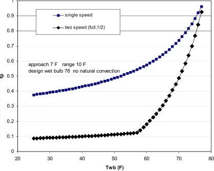
Figure 4.1 shows how fan power changes with ambient wet-bulb temperature for a
counter-flow tower that operates with a constant load. This is a hypothetical case that
neglects natural convection when the fan is off. The upper curve is for on-off fan cycling.
When Tawb = 52 °F, the fan operates one half of the time, and the average power requirement is one half of the rated fan power. The lower curve is for a two-speed fan motor. When Tawb
= 58 °F, the two-speed motor operates at half speed and uses one-eighth of the rated fan
power. When Tawb is above 58 °F, the motor cycles between full speed and half speed.
When Tawb is below 58 °F, the motor cycles between half speed and off. The electrical savings made possible by the two-speed motor can be determined from the difference
between the two curves in Figure 4.1.
Natural convection is accounted for in Figure 4.2. With on-off cycling at Tawb = 52
the fan is off. Thus, it helps the tower with on-off cycling over the entire temperature range.
It has no effect on the two-speed fan until Tawb drops below 58 °F. At lower temperatures, the average power of the two-speed motor is low, and the potential for savings is relatively
small. Thus, the overall effect of natural convection is to reduce the advantage of the
two-speed fan. This is apparent from the smaller area between the curves of Figure 4.2.
Figure 4.3 compares the fan motor power requirements for a counter-flow cooling
tower operating with a constant load. For this case, the motor that operates at 2/3 rated speed
is better at ambient wet-bulb temperatures above 62 °F while the motor that operates at half
speed is better at ambient wet-bulb temperatures below 62 °F.
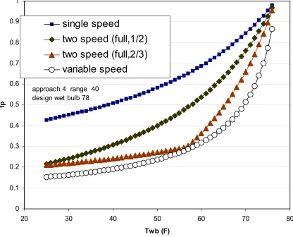
Figure 4.4 compares several control alternatives for a case when the range is
relatively large. The hot water enters the tower at 122 °F throughout the year, and the fans
cycle to maintain the water outlet temperature at 82 °F. The 2/3-speed motor is better than
the half-speed motor for wet-bulb temperatures above about 24 °F in this application, and is almost as good as the motor with a variable speed drive. When the range is large, the mean
temperature difference between the water and the air is not strongly dependent on the
ambient conditions. The heat transfer rate at moderate ambient conditions is not much
greater than the rate at hot conditions. In Figure 4.4 the single-speed motor still runs half of
0 0.1 0.2 0.3 0.4 0.5 0.6 0.7 0.8 0.9 1
20 30 40 50 60 70 80
Twb (F)
fp
single speed two speed (full,1/2)
approach 7 F range 10 F
design wet bulb 78 no natural convection
0 0.1 0.2 0.3 0.4 0.5 0.6 0.7 0.8 0.9 1
20 30 40 50 60 70 80
Twb(F)
fp
single speed
two speed (full,1/2)
approach 7 range 10
design wet bulb 78 nominal case
0 0.1 0.2 0.3 0.4 0.5 0.6 0.7 0.8 0.9 1
20 30 40 50 60 70 80
Twb (F)
fp
single speed
two speed (full,1/2)
two speed (full,2/3)
approach 7 range 10
design wet bulb 78 nominal case
0 0.1 0.2 0.3 0.4 0.5 0.6 0.7 0.8 0.9 1
20 30 40 50 60 70 80
Twb (F)
fp
single speed
two speed (full,1/2)
two speed (full,2/3)
variable speed
approach 4 range 40 design wet bulb 78
4.2 Constant Load Applications
The effect of range on annual fan energy requirements for a counter-flow tower is
shown in Figure 4.5. The results are for a system that returns cold water at 85 °F throughout the year. The entering hot water temperature is also constant, and depends on the range. The
cooling tower is a counter-flow designed for efficiency, c = 3, n = 0.4, C0 = 0.134, operating
in moderate climatic conditions. The fan power at nominal design conditions is 0.0455 hp
per nominal ton, which is typical for this type of tower. The figure shows that the fan electric
energy consumption increases with range. This increase is because the fan remains on for
longer periods of time during the winter, as shown in Figure 4.4. The potential savings,
which depend on the differences between the various curves, are not strongly dependent on
range for this climate. At each range evaluated for this tower, climate, and approach, the
two-speed motor that can run at 2/3 speed consumes less energy during a typical year than
the two-speed motor that can run at 1/2 speed. As expected the motor with the variable speed
drive consumes the least energy of any fan control option. The advantage of the two-speed
(full, 2/3) motor over the two-speed (full, 1/2) motor increases as the range increases.
An electric motor efficiency of 0.90 is factored into the yearly usage and savings data
presented in this paper. Variable speed drive losses, belt drive losses, and the typically lower
efficiency of a two-speed motor at the slower speed are neglected. These assumptions should
not impact the results substantially. For a particular application, known efficiencies can
Table 4.1 lists the energy requirements for a single-speed fan motor and the annual
savings for different capacity control options at several values of range and approach. The
fan with a variable speed drive saves between 52% and 62% of the electricity of a fan that
cycles on and off except in the two cases evaluated with approach above 7 °F. At approach
of 20 °F and range of 10 °F, the variable speed drive savings drop to 35% of the single-speed fan usage. Comparing the savings available between the two-speed fan motor options listed
in Table 1, the two-speed (full, 2/3) is better than the two-speed (full, 1/2) in every operating
condition evaluated except one with savings as much as 76% higher. In the one case where
the two-speed (full, 1/2) has the advantage, the savings are 5% higher. The potential for fan
energy savings decreases at approach temperatures above about 12 °F, and increases slightly as the range increases. The opportunity for savings is a little higher for counter-flow towers
than for cross-flow towers.
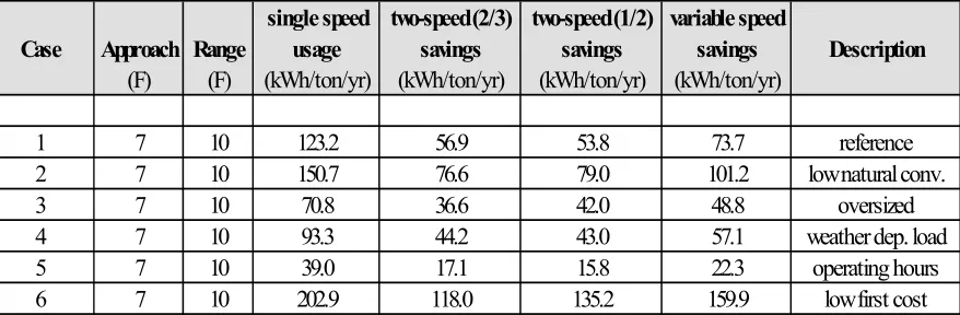
Table 4.2 shows the effects of load variations and tower design variations not
considered in Table 4.1. All of the cases in Table 4.2 have an approach of 7 °F. Cases 1, 2,
5, and 6 have a range of 10 °F. The range is modified in Cases 3 and 4 as described. The savings listed are the difference between the electrical energy requirements of a tower
operating with on-off fan cycling and a tower operating with a two-speed or variable speed
fan. Case 1 is listed for reference purposes. It is a constant load case for an energy efficient
tower. Case 2 is for a tower that has half as much airflow due to natural convection. The
high potential savings for Case 2 demonstrate the importance of natural convection to energy
Case 3 applies to a plant in which a manufacturing process has been eliminated so as
to reduce the load on the cooling tower by one-third. As a result, the cooling tower is
oversized, and the fan cycles on and off even during the hottest day of the summer. The
results show that there is less benefit from two-speed or variable speed fans for this case.
Interestingly, this operating condition favors a two-speed motor that operates at half of its
rated speed.
In all of the cases considered to this point, the load has been held constant throughout
the year. However, even with a constant heat load from process equipment, the load on the
cooling tower may decrease in the winter due to line losses. To model this type of load, the
entering hot water temperature was programmed to change in accordance with the ambient
dry bulb temperature, Ta. For Case 4, a linear relationship between Twi and Ta is assumed.
The load on the tower is reduced by one-half on the coldest day of the winter.
Case 5 is for a plant that operates one shift, five days per week. The cooling tower is
assumed to operate between 7 AM and 5 PM. The results show that the potential energy
savings are reduced roughly in proportion to the operating hours. Daytime wet-bulb
temperatures are usually higher than at night so the tower energy usage and potential savings
are slightly above a proportional reduction according to hours only (about 30% versus 24%).
Case 6 applies to a tower designed for low initial cost. The fan power for this case is
0.0625 hp per nominal ton, and c = 1.33. Opportunities for energy savings increase
20 40 60 80 100 120 140 160 180 200
5 10 15 20 25 30 35 40 45
range (F)
us
ag
e
(k
W
h
/t
on/
yr
)
single speed
two speed (full,2/3)
two speed (full,1/2)
variable speed
Approach 7 F Counterflow
TABLE 4.1 – FAN ENERGY SAVINGS FOR CONSTANT LOAD RALEIGH, NC
single speed two-speed (2/3) two-speed (1/2) variable speed Type Approach Range usage savings savings savings
(F) (F) (kWh/ton/yr) (kWh/ton/yr) (kWh/ton/yr) (kWh/ton/yr)
counter-flow 7 10 123.2 56.9 53.8 73.7
counter-flow 7 15 143.5 65.0 57.5 83.4
counter-flow 7 20 157.6 69.8 57.9 89.1
counter-flow 7 30 172.7 73.7 52.8 93.8
counter-flow 7 40 179.5 72.5 43.4 92.9
counter-flow 4 10 92.9 48.4 51.0 63.1
counter-flow 7 10 123.2 56.9 53.8 73.7
counter-flow 12 10 155.9 58.7 47.8 76.4
counter-flow 20 10 190.1 49.5 28.1 66.9
cross-flow 7 10 95.0 46.4 45.6 59.1
cross-flow 7 15 110.0 53.6 50.0 67.6
cross-flow 7 20 121.5 58.7 52.4 73.7
cross-flow 7 30 136.5 64.3 53.0 80.5
cross-flow 7 40 143.2 66.2 50.3 82.6
TABLE 4.2 – FAN ENERGY SAVINGS FOR COUNTERFLOW TOWERS RALEIGH, NC
single speed two-speed (2/3) two-speed (1/2) variable speed
Case Approach Range usage savings savings savings Description
(F) (F) (kWh/ton/yr) (kWh/ton/yr) (kWh/ton/yr) (kWh/ton/yr)
1 7 10 123.2 56.9 53.8 73.7 reference
2 7 10 150.7 76.6 79.0 101.2 low natural conv.
3 7 10 70.8 36.6 42.0 48.8 oversized
4 7 10 93.3 44.2 43.0 57.1 weather dep. load
5 7 10 39.0 17.1 15.8 22.3 operating hours
4.3 Similar Applications in Various Climates
The impact of climate on cooling tower fan energy usage and potential energy
savings is estimated using typical meteorological year data for five locations listed in Table
4.3. The fan energy savings in this table represent a tower characterized by Equation (6) with
c = 3 and n = 0.40. The heat transfer by natural convection is calculated from Equation (10),
assuming C0 = 0.134. The fan power is 0.0455 hp/ton. In each case, the load is held constant
throughout the year. It is assumed that the tower is correctly sized for the load so that the fan
does not cycle at design point conditions. The design point wet-bulb temperature for each
city is listed in the table.
The energy savings in Table 4.3 are for a counter-flow tower that operates with a
steady load for 8760 hours per year. As an approximation, the savings for towers that operate
fewer hours can be reduced in proportion to the operating hours. For the towers and
operating conditions represented in Table 4.3, fan motors that operate at 2/3 speed save more
energy than motors that operate at 1/2 speed. The advantage of the two-speed (full, 2/3) fan
motors over the two-speed (full, 1/2) increases as the range increases, as the approach
increases, and is more pronounced in some locations.
For variable speed motors and for motors that run at 2/3 speed, the potential savings
are insensitive to the approach temperature in every location. However, it is expected that
Houston, the potential savings are insensitive to range. In Raleigh, and to a larger extent, in
Columbus and Denver, the savings increase with range.
The cities in Table 4.3 are arranged in order of decreasing design wet-bulb
temperature. By examination of the results, it is apparent that the single-speed usage and
potential savings for various fan speed options is unrelated to the design wet-bulb
temperature. In order to study the effect of climate on the results, the mean wet-bulb
temperature for the typical meteorological year data was calculated and compared to the
design wet-bulb temperature at each location. The location with the smallest difference
between mean wet-bulb and design wet-bulb and consequently the highest single speed
energy consumption is Los Angeles. Figure 4.6 is a plot of single-speed usage from Table
4.3 versus location with the locations arranged in order of increasing difference between
mean wet-bulb temperature and design wet-bulb temperature. This plot shows a good
correlation between cooling tower single-speed fan motor consumption and the difference
between design wet-bulb temperature and mean wet-bulb temperature for a particular
location.
Figure 4.7 is a plot of potential fan energy savings at nominal conditions versus
location. The locations are arranged in order of increasing difference between design
wet-bulb temperature and mean wet-wet-bulb (increasing single-speed fan motor consumption). This
plot shows that for this tower and operating conditions the locations with the highest
consumption generally have the highest potential savings and the type of two-speed fan with
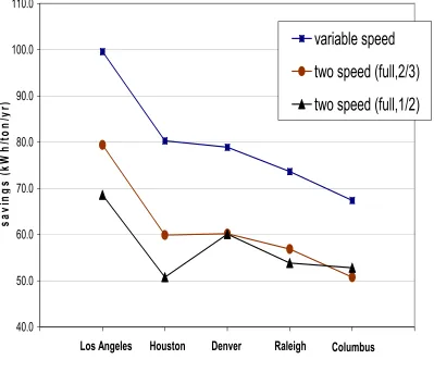
Figure 4.8 plots the potential savings for alternative capacity control methods for
various locations when the range is 40 °F and the approach is 7 °F. The fan motors that operate at 2/3 speed are more energy efficient than the motors that operate at 1/2 speed for
each location. The plot shows that in general the advantage for the 2/3 speed motor over the
1/2 speed motor increases as the range increases.
In Figure 4.8, the locations are again arranged in order of increasing difference
between design wet-bulb temperature and mean wet-bulb (increasing single-speed fan motor
consumption). Under these operating conditions, the correlation between the most savings
being available for the towers with the highest consumption begins to break down. In
particular, the potential savings for Houston are much less than the other locations as a
percentage of single-speed fan motor usage. To investigate, the standard deviation of the
hourly wet-bulb temperatures was calculated for each location’s typical meteorological year
data and compared to the difference between the design wet-bulb temperature and the mean
wet-bulb temperature. The location where the standard deviation is closest to the difference
in design and mean wet-bulb is Houston. The standard deviation being close to the
difference in design and mean wet-bulb suggests that the wet-bulb temperature is relatively
often near the design wet-bulb and, likewise, relatively often far below the design wet-bulb.
These conditions limit the amount of savings available for the fan speed control options. In
Figure 4.9, the distributions of hourly wet-bulb temperatures during a typical year are shown
for the subject climates with the highest (Columbus) and the lowest (Houston) percentage
Figure 4.10 plots the variable speed savings as a percentage of single-speed motor
consumption for various operating conditions with the locations arranged in order of
increasing difference between design wet-bulb minus mean wet-bulb and standard deviation.
This plot shows a good correlation between percent savings and this parameter. Also, where
the wet-bulb is relatively often near the design wet-bulb, the two-speed (full, 2/3) should
have the advantage over the two-speed (full, 1/2). Results in Table 4.3 show that the
locations where the two-speed (full, 2/3) is most advantageous are Houston and Los Angeles.
Figure 4.11 shows that the 1/2 speed fan is better than the 2/3 speed fan for cooling
towers designed for low initial costs with moderate loads (range = 10 F). However, as the
range increases, the 2/3 speed fan becomes more advantageous relative to the 1/2 speed fan.
Figure 4.12 shows that the best choice for towers designed for low initial cost is dependent
on location for high loads (range = 40 F).
The savings in Table 4.3 are in the range of 50 to 100 kWh/ton/yr. For a fan power of
0.0455 hp/ton, a small tower with a 1 hp fan would have a nominal capacity of about 22 tons.
Thus, the electrical energy savings for the small tower would be in the range of 1100 to 2200
kWh/yr. If electricity cost $.05/kWh, the dollar savings are in the range of $55/yr to $110/yr.
The dollar savings for a 1650-ton tower with a 75 hp motor are in the range of $4100/yr to
TABLE 4.3 – FAN ENERGY SAVINGS FOR VARIOUS LOCATIONS
Design single speed two-speed (2/3) two-speed (1/2) variable speed City Wet Bulb Approach Range usage savings savings savings
(F) (F) (F) (kWh/ton/yr) (kWh/ton/yr) (kWh/ton/yr) (kWh/ton/yr)
Houston 79 7 10 160.5 59.9 50.8 80.3
79 7 40 204.4 60.9 32.4 84.6
79 12 10 189.1 53.2 38.0 73.0
Raleigh 78 7 10 123.2 56.9 53.8 73.7
78 7 40 179.5 72.5 43.4 92.9
78 12 10 155.9 58.7 47.8 76.4
Columbus 75 7 10 111.1 50.8 52.8 67.4
75 7 40 172.3 75.6 50.1 93.2
75 12 10 145.1 58.2 51.5 75.0
Los Angeles 69 7 10 168.4 79.4 68.6 99.6
69 7 40 219.1 84.8 42.7 109.1
69 12 10 196.6 73.1 46.1 91.1
Denver 63 7 10 134.0 60.2 60.1 78.9
63 7 40 194.8 84.1 59.6 104.9
100.0 120.0 140.0 160.0 180.0 200.0 220.0 240.0
10 12 14 16 18 20 22 24 26 28 30
design WB - mean WB (F)
si n g le -s p ee d U sa g e (k W h/ ton/ yr )
approach 7, range 40
approach 12, range 10
approach 7, range 10
Los Angeles Houston
Denver Raleigh
Columbus
40.0 50.0 60.0 70.0 80.0 90.0 100.0 110.0
0 1 2 3 4 5 6
sa
vi
n
g
s
(k
W
h/
to
n/
yr
)
variable speed
two speed (full,2/3)
two speed (full,1/2)
Denver
Los Angeles Houston Raleigh Columbus
30 40 50 60 70 80 90 100 110 120
0 1 2 3 4 5 6
s
avi
n
g
s
(kW
h
/t
o
n
/y
r)
variable speed
two speed (full,2/3)
two speed (full,1/2)
Denver
Los Angeles Houston Raleigh Columbus
0 100 200 300 400 500 600
0 10 20 30 40 50 60 70 80 90
hourly wet-bulb (F)
o
ccu
re
n
c
es i
n
o
n
e y
ear
Columbus, Ohio
Houston, Texas
30 35 40 45 50 55 60 65
2 4 6 8 10 12 14
[design WB - mean WB]-std dev WB (F)
va ri ab le s p ee d d ri ve s avi n g s (% )
approach 7, range 40
approach 12, range 10
approach 7, range 10
Los Angeles Houston
Denver
Raleigh Columbus
FIGURE 4.10 - VARIABLE SPEED DRIVE SAVINGS AS PERCENTAGE OF SINGLE-SPEED CONSUMPTION FOR VARIOUS LOCATIONS AND OPERATING
100.0 110.0 120.0 130.0 140.0 150.0 160.0 170.0 180.0 190.0 200.0
0 1 2 3 4 5 6
sav
in
g
s
(k
W
h/
ton/
yr
)
variable speed
two speed (full,1/2)
two speed (full,2/3)
Denver
Los Angeles Houston Raleigh Columbus
140.0 150.0 160.0 170.0 180.0 190.0 200.0 210.0 220.0 230.0 240.0
0 1 2 3 4 5 6
s
avi
n
g
s
(kW
h
/t
o
n
/y
r)
variable speed
two speed (full,1/2)
two speed (full,2/3)
Denver
Los Angeles Houston Raleigh Columbus
4.4 Ideal Second Speed
The parametric analysis of the effects of both the climate and the operating conditions
(load, approach) has shown a clear advantage of different speeds in certain applications.
These findings suggest that an ideal second speed can be found that maximizes savings for
the two-speed fan control option. Two-speed motors are readily available only in discrete
steps with the slower speed usually 1/2 or 2/3 of full speed. This fact limits from a practical
standpoint the slower speed that is used. Typically the slower speed in commercial cooling
towers is either 1/2 or 2/3 full speed depending on the manufacturer. There is one design that
allows selection of any speed easily. This design uses a second independent motor called a
pony motor that is connected to drive the fan shaft by a separate belt and pulley. With this
configuration, the cooling tower could be tuned to a specific application in a specific climate
by selecting the ideal second speed. To investigate the dependence of savings on the
selected second speed, energy usages were calculated over a range of second speeds for the
nominal case and several cases for which savings seemed to be particularly sensitive to the
slower speed. Figure 4.13 shows that the ideal second speed for a two-speed fan varied from
1/2 to 3/4 for the particular towers and applications represented. It is expected that the ideal
0.0 20.0 40.0 60.0 80.0 100.0 120.0 140.0 160.0
0.200 0.300 0.400 0.500 0.600 0.700 0.800 0.900
second speed
sa
vi
n
g
s
(k
W
h/
ton/
yr
)
nominal Raleigh 7/10
nominal Houston 7/40
low cost Raleigh 7/10
4.5 Comparison of Equipment Cost and Estimated Savings
The cost for installing two-speed motors or variable speed drives on cooling towers
depends somewhat on the cooling tower capacity. A single-speed 1hp motor for a small
tower might cost $150/hp, while a 75 hp motor for a large tower might cost only $50/hp.
Two-speed motors can be expected to cost twice as much. Variable speed drives will
probably cost $800/hp for small motors and $200/hp for large motors.
Thus, the cost to replace a 1 hp single-speed fan motor with a two-speed motor would
probably be in the range of $500. The payback period is 5 to 10 years. The cost to replace
the single-speed 75 hp motor is probably in the range of $7500, and the payback period is in
the range of 1 to 2 years. For smaller towers with belt driven fans, the most cost effective
solution is to install a second motor to drive the fan at slower speed. For example, a tower
with a 25 hp motor would require a 7.5 hp motor to drive the fan at 2/3 speed. The
economics will be better in locations where the cost of electricity is higher than $.05/kWh,
and for towers with small heat transfer areas for which the nominal fan power would be
considerably greater than 0.0455 hp/ton. The economics will be worse for plants that operate
one shift and in plants where the tower is oversized.
5.0 Conclusions
Calculations based on typical meteorological year data show that fan energy savings
for alternative capacity control methods do not depend strongly on the approach temperature.
In colder climates, the potential savings increase by 25% to 40% when the range increases
convection that occurs when the fan is off. The greatest potential for savings occurs in
towers designed for low cost. The fan power for such a tower would be in the range of 0.08
hp/nominal-ton, and the airflow due to natural convection would be small in comparison to
the fan capacity. A tower with a fan power of 0.04 hp/ton benefits more from natural
convection, and has less potential for energy savings. There is less potential for savings in
cross-flow towers than in counter-flow towers. Also, the potential savings are lower when
the cooling tower is oversized, or when the plant operates one shift instead of three shifts.
Two-speed fans that operate at 1/2 of the rated speed are suitable for low cost towers
at moderate loads. Two- speed fans that operate at 2/3 of the rated speed are a better choice
for energy efficient towers in most locations, especially at higher operating loads. At
nominal conditions of approach = 7 °F and range = 10 °F, the single-speed energy usage and thus the potential savings are highest in locations where the wet-bulb temperature remains
close to the design value through much of the year. The potential energy savings at nominal
conditions in Los Angeles are about 50% higher than the savings in Columbus, Ohio. As a
percentage of the single-speed fan energy usage, potential savings are a function of the
distribution of the wet-bulb temperatures during the year.
6.0 References
1. Typical Meteorological Year Data. National Climatic Center, Asheville, NC.
2. Stout, M.R., J.W. Leach. 2001. “Cooling Tower Fan Control for Energy Efficiency.” Energy Engineering, Volume 99, Number 1/December-January 2002.
4. Braun, J.E., G.T. Diderrich. 1990. “Near-Optimal Control of Cooling Towers for Chilled-Water Systems.” ASHRAE Transactions, Vol. 96, Part 2.
5. Hensley, J.C. “The Application of Cooling Towers for Free Cooling.” ASHRAE Transactions: Symposia, No-94-7-3, page 817.
6. ICT Cooling Towers, Bulletin 340C. Published by EVAPCO Inc., Westminster, Maryland.
7. Industrial Modular Cooling Towers, Bulletin 5735/1-OBA. Published by Baltimore Aircoil Company, Baltimore, MD.
8. Series V Cooling Towers, Bulletin S282/1-OEA. Published by Baltimore Aircoil Company, Baltimore, MD.
9. Hensley, J.C. Cooling Tower Fundamentals. Published by The Marley Cooling Tower Company, Mission, Kansas. Page 72.
10. Braun, J.E., S.A. Klein, and J.W. Mitchell. 1989. “Effectiveness Models for Cooling Towers and Cooling Coils.” ASHRAE Transactions, Vol. 95, Part 2.
11. Hill, G.B., E.J. Pring, and P.D. Osborn. 1990. Cooling Towers, Principles and Practice. Butterworth-Heineann, London. Page 149.
12. Baker, D. 1984. Cooling Tower Performance. Chemical Publishing Company, New York. Page 140.
c Single Point Operation - Counterflow dimension tout(4)
100 format(5F8.3)
open(unit=11,file="data",status="old")
write(*,*) 'enter range, approach, ratio,designWB' read(*,*) range,approach,ratio,twbd
write(11,*) 'approach',approach,' range',range write(11,*) 'design wet bulb',twbd
write(11,*) ' wetbulb-hp1-hp23-hp12-hpv' two=twbd+approach
twi=two+range do 10 i=1,53 twb=24.+i tdb=twb tdp=twb
c write(*,*)' enter tdb,tdp,twi,ratio' c read(*,*) tdb,tdp,twi,ratio
call cycle(tdb,tdp,twi,ratio,tout)
c write(*,*) 'two ',tout(1),tout(2),tout(3),tout(4) f=(two-tout(1))/(tout(4)-tout(1))
hp1=f
IF (two.lt.tout(3)) THEN
f=(two-tout(3))/(tout(4)-tout(3)) hp23=f+(1-f)*(.667**3.) ELSE f=(two-tout(1))/(tout(3)-tout(1)) hp23=f*(.667**3.) END IF
IF (two.lt.tout(2)) THEN
f=(two-tout(2))/(tout(4)-tout(2)) hp12=f+(1-f)*(.5**3.) ELSE f=(two-tout(1))/(tout(2)-tout(1)) hp12=f*(.5**3.) END IF call vspeed(tdb,tdp,twi,ratio,two,f) hpv=f**3.
10 write(11,100) twb,hp1,hp23,hp12,hpv stop end subroutine vspeed(tai,tdp,twi,ratio,twout,f) dimension cfm(2),diff(2) astd=990. wmdoti=astd/ratio c=3. call psych(tai,tdp,wai,hai) call psych(twi,twi,wwi,hwi) cfm(1)=13400. cfm(2)=1340. count=0.
5 count=count+1. do 20 i=1,2
v=.02519*(1.+1.61*wai)*(tai+460.)/(1.+wai) do 10 k=1,3
xntu=c*(wmdoti/amdot)**.4
call ctower(amdot,tai,tdp,wmdoti,twi,xntu,two,wmdoto,wao,hao) call psych(two,two,wwo,hwo)
twbo=14.24+1.43*hao
10 v=.02519*(1.+1.61*wao)*(twbo+460.)/(1.+wao) 20 diff(i)=twout-two
cfm(2)=(cfm(2)*diff(1)-cfm(1)*diff(2))/(diff(1)-diff(2)) cfm(1)=.98*cfm(2)
test=abs(diff(2))
if(count.gt.10) write(*,*)'vspeed failed' if(count.gt.10) go to 30
if(test.gt..01) go to 5 30 f=cfm(2)/13400.
return end subroutine cycle(tai,tdp,twi,ratio,tout) dimension tout(4),cfm(4) astd=990. wmdoti=astd/ratio xntu=3. c=3. call psych(tai,tdp,wai,hai) call psych(twi,twi,wwi,hwi) dh=hwi-hai v=.02519*(1.+1.61*wai)*(tai+460.)/(1.+wai) do 10 k=1,3
cfm0=2000.*dh**.20 amdot=cfm0/v call ctower(amdot,tai,tdp,wmdoti,twi,xntu,two,wmdoto,wao,hao) call psych(two,two,wwo,hwo) twbo=14.24+1.43*hao v=.02519*(1.+1.61*wao)*(twbo+460.)/(1.+wao) dti=hwo-hai dto=hwi-hao dh=(dti-dto)/alog(dti/dto) 10 tout(1)=two
cfm(2)=13200./2. cfm(3)=13200.*2./3. cfm(4)=13200.
do 30 n=2,4
v=.02519*(1.+1.61*wai)*(tai+460.)/(1.+wai) do 20 k=1,3
amdot=cfm(n)/v
xntu=c*(wmdoti/amdot)**.4
call ctower(amdot,tai,tdp,wmdoti,twi,xntu,two,wmdoto,wao,hao) twbo=14.24+1.43*hao
20 v=.02519*(1.+1.61*wao)*(twbo+460.)/(1.+wao) 30 tout(n)=two
return end subroutine ctower(amdot,tai,tdp,wi,twi,xntu,two,wo,wao,hao) dimension tsw(2),diff(2) wmdoti=wi call psych(tai,tdp,wai,hai) call psych(twi,twi,wswi,hswi) tsw(1)=(tai+tdp)/2. tsw(2)=tsw(1)+1. count=0.
10 count=count+1 do 20 i=1,2 twb=tsw(i)
call psych(twb,twb,wwb,hwb) 20 diff(i)=hai-hwb
tsw(2)=(tsw(1)*diff(2)-tsw(2)*diff(1))/(diff(2)-diff(1)) tsw(1)=tsw(2)-1.
if(count.gt.10) write(*,*) 'twb failed' if(count.gt.10) go to 30
test=abs(diff(2))/hai if(test.gt..0005) go to 10 30 two=twb
c write(*,*)' twb,hwb =',twb,hwb
c write(*,*)'approx water outlet temp. =',two do 70 j=1,5
call psych(two,two,wswo,hswo) cs=(hswi-hswo)/(twi-two) smdot=amdot*cs/wmdoti texp=exp(xntu*(smdot-1.)) eff=(1.-texp)/(1.-smdot*texp) hao=hai+eff*(hswi-hai) hswe=hai+(hao-hai)/(1.-exp(-xntu)) tsw(1)=(twi+two)/2. tsw(2)=tsw(1)+1. count=0.
40 count=count+1 do 50 i=1,2 ta=tsw(i)
call psych(ta,ta,wswe,h) 50 diff(i)=hswe-h
tsw(2)=(tsw(1)*diff(2)-tsw(2)*diff(1))/(diff(2)-diff(1)) tsw(1)=tsw(2)-1.
if(count.gt.10) write(*,*) 'hswe failed' if(count.gt.10) go to 60
test=abs(diff(2))/hswe if(test.gt..0005) go to 40 60 wao=wswe+(wai-wswe)/exp(xntu) wmdoto=wmdoti-amdot*(wao-wai)
70 two=32.+(wmdoti*(twi-32.)-amdot*(hao-hai))/wmdoto eff2=(twi-two)/(twi-twb)
evap=(wmdoti-wmdoto)/wmdoti wo=wmdoto
************************************************************************** ******PROGRAM ESTIMATES YEARLY COOLING TOWER FAN ENERGY REQUIREMENTS USING ******DIFFERENT CAPACITY CONTROL OPTIONS - SINGLE SPEED MOTOR, TWO SPEED ******MOTORS (ONE-HALF AND TWO-THIRDS SPEED), AND VARIABLE SPEED
dimension tout(4),hp(4) 100 format(I4,3F8.2)
******ACCESS HOURLY TMY DATA FILE AND SET DESIGN PARAMETERS FOR THE ******COOLING TOWER, SUM VARIABLES USED TO SUM HP REQUIREMENTS open(unit=11,file="hou.dat",status="old")
write(*,*) 'enter range, approach, ratio,designWB' read(*,*) range,approach,ratio,twbd sum1=0. sum23=0. sum12=0. sumv=0. two=twbd+approach twi=two+range do 10 i=1,8760
read(11,100) nhr,tdb,tdp,twb
call cycle(tdb,tdp,twi,ratio,tout,hp) IF (tout(1).lt.two) THEN
hp(1)=0. hp(2)=0. hp(3)=0. hp(4)=0. END IF f=(two-tout(1))/(tout(4)-tout(1)) hp1=f*hp(4) sum1=hp1+sum1
IF (two.lt.tout(3)) THEN
f=(two-tout(3))/(tout(4)-tout(3)) hp23=f*hp(4)+(1-f)*hp(3) ELSE f=(two-tout(1))/(tout(3)-tout(1)) hp23=f*hp(3) END IF sum23=hp23+sum23
IF (two.lt.tout(2)) THEN
f=(two-tout(2))/(tout(4)-tout(2)) hp12=f*hp(4)+(1-f)*hp(2) ELSE f=(two-tout(1))/(tout(2)-tout(1)) hp12=f*hp(2) END IF sum12=hp12+sum12 call vspeed(tdb,tdp,twi,ratio,two,f,hpv) IF (tout(1).lt.two) THEN
hpv=0. END IF
10 sumv=hpv+sumv
write(*,*) ' design wet bulb approach range hours' write(*,*) twbd,approach,range,nhr
write(*,*) ' sum1 sum23 sum12 sumv ' write(*,*) sum1,sum23,sum12,sumv
end
************************************************************************** ******SUBROUTINE TO DETERMINE HP REQUIREMENT FOR VARIABLE SPEED FAN MOTOR ******OPTION. USES TRIAL AND ERROR TO FIND CFM THAT WILL MATCH DESIRED ******COLD WATER OUT TEMPERATURE. ASSUMES FAN LAW TO DETERMINE HP ******REQUIREMENT. subroutine vspeed(tai,tdp,twi,ratio,twout,f,hpv) dimension cfm(2),diff(2) astd=990. wmdoti=astd/ratio c=3. call psych(tai,tdp,wai,hai) call psych(twi,twi,wwi,hwi) cfm(1)=13200. cfm(2)=1320. count=0.
5 count=count+1. do 20 i=1,2
v=.02519*(1.+1.61*wai)*(tai+460.)/(1.+wai) do 10 k=1,3
amdot=cfm(i)/v
xntu=c*(wmdoti/amdot)**.4
call ctower(amdot,tai,tdp,wmdoti,twi,xntu,two,wmdoto,wao,hao) call psych(two,two,wwo,hwo)
twbo=14.24+1.43*hao
10 v=.02519*(1.+1.61*wao)*(twbo+460.)/(1.+wao) 20 diff(i)=twout-two
cfm(2)=(cfm(2)*diff(1)-cfm(1)*diff(2))/(diff(1)-diff(2)) cfm(1)=.98*cfm(2)
test=abs(diff(2))
if(count.gt.10) write(*,*)'vspeed failed' if(count.gt.10) go to 30
if(test.gt..01) go to 5 30 f=cfm(2)/13200.
hpv=13.33/v*f**3. return
end
************************************************************************** ******SUBROUTINE TO DETERMINE HP REQUIREMENT FOR SINGLE SPEED AND TWO ******SPEED FANS. DETERMINES COLD WATER TEMPERATURE FOR THE PERTINENT CFM ******BASED ON SPEEDS AND THE FAN LAWS. SEEKS AVERAGE COLD WATER
******TEMPERATURE TO MATCH DESIRED COLD WATER TEMPERATURE. ASSUMES FAN ******LAW TO DETERMINE HP REQUIREMENT
subroutine cycle(tai,tdp,twi,ratio,tout,hp) dimension tout(4),cfm(4),hp(4) astd=990. wmdoti=astd/ratio xntu=3.2 c=3. call psych(tai,tdp,wai,hai) call psych(twi,twi,wwi,hwi) dh=hwi-hai v=.02519*(1.+1.61*wai)*(tai+460.)/(1.+wai) do 10 k=1,3
amdot=cfm0/v call ctower(amdot,tai,tdp,wmdoti,twi,xntu,two,wmdoto,wao,hao) call psych(two,two,wwo,hwo) twbo=14.24+1.43*hao v=.02519*(1.+1.61*wao)*(twbo+460.)/(1.+wao) dti=hwo-hai dto=hwi-hao dh=(dti-dto)/alog(dti/dto) 10 tout(1)=two
cfm(2)=13200.*6./12. cfm(3)=13200.*8./12. cfm(4)=13200.
do 30 n=2,4
v=.02519*(1.+1.61*wai)*(tai+460.)/(1.+wai) do 20 k=1,3
amdot=cfm(n)/v
xntu=c*(wmdoti/amdot)**.4
call ctower(amdot,tai,tdp,wmdoti,twi,xntu,two,wmdoto,wao,hao) twbo=14.24+1.43*hao
20 v=.02519*(1.+1.61*wao)*(twbo+460.)/(1.+wao) hp(n)=13.33/v*(cfm(n)/13200)**3
30 tout(n)=two return end
************************************************************************** ******SUBROUTINE TO DETERMINE HUMIDITY RATIO AND ENTHALPY OF AIR BASED ON ******EMPIRICAL RELATIONSHIPS GIVEN AMBIENT TEMPERATURE AND DEWPOINT ******TEMPERATURE subroutine psych(ta,tdp,w,h) psat=exp(14.8305-7362.08/(tdp+394.67)) y=psat/14.696 w=.6219*y/(1.-y) h=.249*(ta-2.5)+1100.*w return end ************************************************************************** ******SUBROUTINE TO DETERMINE COOLING TOWER EXIT WATER TEMPERATURE, EXIT ******WATER MASS FLOWRATE, EXIT AIR SPECIFIC HUMIDITY, AND EXIT AIR
******ENTHALPLY GIVEN ENTERING WATER TEMPERATURE, AMBIENT AIR CONDITIONS, ******COOLING TOWER NTU'S, AND ENTERING WATER AND AIR MASS FLOWRATES subroutine ctower(amdot,tai,tdp,wi,twi,xntu,two,wo,wao,hao) dimension tsw(2),diff(2) wmdoti=wi call psych(tai,tdp,wai,hai) call psych(twi,twi,wswi,hswi) tsw(1)=(tai+tdp)/2. tsw(2)=tsw(1)+1. count=0.
10 count=count+1 do 20 i=1,2 twb=tsw(i)
call psych(twb,twb,wwb,hwb) 20 diff(i)=hai-hwb
if(count.gt.10) write(*,*) 'twb failed' if(count.gt.10) go to 30
test=abs(diff(2))/hai if(test.gt..0005) go to 10 30 two=twb
c write(*,*)' twb,hwb =',twb,hwb
c write(*,*)'approx water outlet temp. =',two do 70 j=1,5
call psych(two,two,wswo,hswo) cs=(hswi-hswo)/(twi-two) smdot=amdot*cs/wmdoti c texp=exp(xntu*(smdot-1.)) c eff=(1.-texp)/(1.-smdot*texp) texp=exp(-xntu) texp=exp(smdot*(texp-1.)) eff=(1.-texp)/smdot hao=hai+eff*(hswi-hai) hswe=hai+(hao-hai)/(1.-exp(-xntu)) tsw(1)=(twi+two)/2. tsw(2)=tsw(1)+1. count=0.
40 count=count+1 do 50 i=1,2 ta=tsw(i)
call psych(ta,ta,wswe,h) 50 diff(i)=hswe-h
tsw(2)=(tsw(1)*diff(2)-tsw(2)*diff(1))/(diff(2)-diff(1)) tsw(1)=tsw(2)-1.
if(count.gt.10) write(*,*) 'hswe failed' if(count.gt.10) go to 60
test=abs(diff(2))/hswe if(test.gt..0005) go to 40 60 wao=wswe+(wai-wswe)/exp(xntu) wmdoto=wmdoti-amdot*(wao-wai)
70 two=32.+(wmdoti*(twi-32.)-amdot*(hao-hai))/wmdoto eff2=(twi-two)/(twi-twb)
evap=(wmdoti-wmdoto)/wmdoti wo=wmdoto