Adaptive Projection Confidence Sets and Data Analyses in Personalized Medicine.

(1)

Abstract

FAN WU. Adaptive Projection Confidence Sets and Data Analyses in Personalized Medicine. (Under the direction of Eric B. Laber.)

(2)

c

(3)

Adaptive Projection Confidence Sets and Data Analyses in Personalized Medicine

by Fan Wu

A dissertation submitted to the Graduate Faculty of North Carolina State University

in partial fulfillment of the requirements for the Degree of

Doctor of Philosophy

Statistics

Raleigh, North Carolina 2016

APPROVED BY:

Leonard Stefanski Dennis Boos

Michael Kosorok Eric Laber

(4)

Dedication

(5)

Biography

(6)

Acknowledgements

First, I would like to thank my thesis advisor Dr. Eric Laber for his kind guidance, inspiration, and continued support during my ph.D. study. When I met problems, he al-ways patiently gave me suggestions, and encouraged me to continue my research projects. I greatly appreciate the time and effort that he dedicated to helping me complete the research projects smoothly.

I would like to thank my committee members Dr. Leonard Stefanski, Dr. Michael Kosorok, and Dr. Dennis Boos constructive comments and suggestions for my research. I especially thank Dr. Stefanski for giving me a lot of suggestions during our lab meetings. His suggestions are really helpful.

I am grateful to my intern supervisor Dr. Ilya Lipchovich, and the collaborated professor Dr. Emanuel Severus. Thanks for their help and effort in the STEP-BD project. Without their guidance, I cannot finish the STEP-BD data analysis in my thesis.

I also thank the lab members from Dr. Laber’s group. They provide me a lot of suggestions in my research work during the weekly group meeting. I also learned a lot of knowledge from different research area through their presentations and discussion during the group meetings.

(7)

LIST OF TABLES

Table 2.1 Monte Carlo estimates of coverage probabilities of confidence inter-vals for the toy example at 95% nominal level. The rows represent different methods of constructing CIs: (i) the n-out-of-n centered percentile bootstrap (CPB); (ii) the projection confidence interval (PCI); (iii) the proposed adaptive projection interval (API). Esti-mates are constructed using 200 datasets, and 500 bootstraps drawn from each dataset. Coverage rate significantly different from 0.95 at the 0.05 level are in bold. The ones that significantly below 0.95 are marked with∗. . . 17 Table 2.2 Monte Carlo estimates of the mean width of confidence intervals for

the toy example at 95% nominal level. The rows represent different methods of constructing CIs: (i) the n-out-of-n centered percentile bootstrap (CPB); (ii) the projection confidence interval (PCI); (iii) the proposed adaptive projection interval (API). estimates are con-structed using 200 datasets, and 500 bootstraps from each dataset. Widths with coverage rate significantly different from 0.95 at the 0.05 level are in bold. The ones with coverage rate significantly below 0.95 are marked with∗. . . 17 Table 2.3 Parameters indexing the example models. Examples are designated

(11)

Table 2.4 Monte Carlo estimates of coverage probabilities of confidence in-tervals for the main effect of treatment at the 95% nominal level. The rows represent different methods of constructing CIs: (i) the n-out-of-n centered percentile bootstrap (CPB); (ii) the projection confidence interval (PCI); (iii) the m-out-of-n bootstrap; (iv) the proposed adaptive projection interval (API). Estimates are con-structed using 200 datasets of size 150 drawn from each model, and 1000 bootstraps drawn from each dataset. Examples are designated NR=nonregular, NNR=near-nonregular, R=regular. . . 24 Table 2.5 Monte Carlo estimates of the mean width of confidence intervals for

the main effect of treatment at the 95% nominal level. The rows represent different methods of constructing CIs: (i) the n-out-of-n centered percentile bootstrap (CPB); (ii) the projection confidence interval (PCI); (iii) the m-out-of-n bootstrap; (iv) the proposed adaptive projection interval (API). Estimates are constructed using 200 datasets of size 150 drawn from each model, and 1000 bootstraps drawn from each dataset. Examples are designated NR=nonregular, NNR=near-nonregular, R=regular. . . 25 Table 3.1 Candidate predictors for regression models in Q-learning. Those

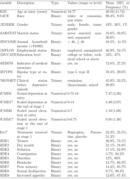
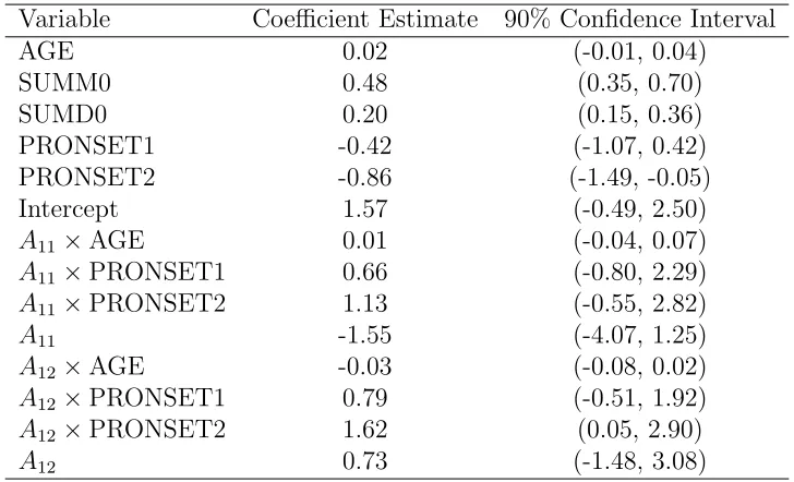
that are only available for the second stage regression model are starred. . . 42 Table 3.2 Point estimates and confidence intervals for the coefficients indexing

the second stage Q-function. . . 43 Table 3.3 Point estimates and confidence intervals for the coefficients indexing

the first stageQ-function. . . 45 Table 3.4 Point estimates and confidence intervals for the expected depression

score SUMD at week 12 under static regimes(first line treatment, second line treatment) and estimated DTR. . . 46 Table 3.5 Antidepressants are divided into 4 groups, and the dosage for each

medication is divided into 3 levels: high, median, and low. . . 50 Table 3.6 Mood-stabilizers are divided into 5 groups, and the dosage for each

(12)

Table 3.7 Part of feasible treatments F(h) in SAD study. It is a combination of treatment T1 and T2. Here the possible combination treatments

regarding Mood 1 are listed. . . 53 Table 3.8 Candidate predictors for regression models inQ-learning. . . 57 Table 3.9 Estimated optimal regime with RACE = 1,MEDINS = 1. Mi,

Aj represent group i mood-stabilizer and group j antidepressant respectively. “Low”, “Medium”, and “High” denote mood-stabilizer and antidepressants dosage levels. . . 58 Table 3.10 Estimated optimal regime with RACE = 1,MEDINS = 0. Mi,

Aj represent group i mood-stabilizer and group j antidepressant respectively. “Low”, “Medium”, and “High” denote mood-stabilizer and antidepressants dosage levels. . . 59 Table 4.1 Dosage assignment situation at each time point. There are 852

patients in total. At each time point, patients may drop off due to the severe adverse events. . . 70 Table 4.2 The estimated optimal treatment regime with different thresholds

τ. β1 andγ are parameters for regimeπ1. β0is the parameter vector

for regimeπ0. . . 71

Table 4.3 Dosage assignment situation at each time point. There are 460 patients in total. At each time point, patients may drop off due to the severe adverse events. . . 73 Table 4.4 The estimated optimal treatment regime with different thresholds

τ. β1 andγ are parameters for regimeπ1. β0is the parameter vector

(13)

Table A.1 The estimated coefficients of mood-stabilizer grouped effect in SAD. α0k represents the kth group defined in Table 3.6. . . 99 Table A.2 The estimated coefficients of antidepressants grouped effect in SAD.

η0k represents the kth group defined in Table 3.5. . . 99 Table A.3 The estimated coefficients of mood-stabilizer dose effect with level

medium in SAD. Note, only Mood 1 and Mood 2 are considered. . 99 Table A.4 The estimated coefficients of mood-stabilizer dose effect with level

high in SAD. Note, only Mood 1 and Mood 2 are considered. . . . 100 Table A.5 The estimated coefficients of treatment effect with each mood-stabilizer

group (δt1) based on Table 3.6. . . 100

Table A.6 The estimated coefficients of antidepressants dose effect with level medium in SAD. . . 100 Table A.7 The estimated coefficients of antidepressants dose effect with level

high in SAD. . . 100 Table A.8 The estimated coefficients of treatment effect with each

(14)

LIST OF FIGURES

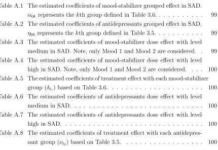
Figure 2.1 Monte Carlo estimates of coverage rates of confidence intervals for the V alue at 95% nominal level. The texts in the plot represent the coverage rate. x-axis and y-axis are values of the two parame-ters c, ρ for generated models. Sample size n = 150, Monte Carlo replication Nrep = 100, and Bootstrap sample size B = 1000. . . 20 Figure 2.2 Monte Carlo estimates of the mean width of confidence intervals

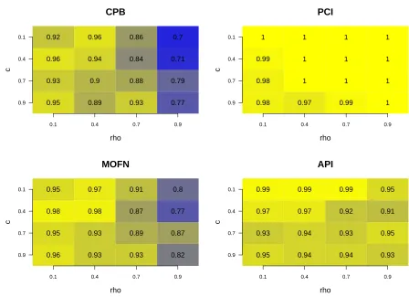
for theV alueat 95% nominal level. The texts in the plot represent the average width of the confidence intervals. x-axis and y-axis are values of the two parameters c, ρ for generated models. Sample size n = 150, Monte Carlo replication Nrep = 100, and Bootstrap sample size B = 1000. . . 21 Figure 2.3 Monte Carlo estimates of coverage rates of confidence intervals for

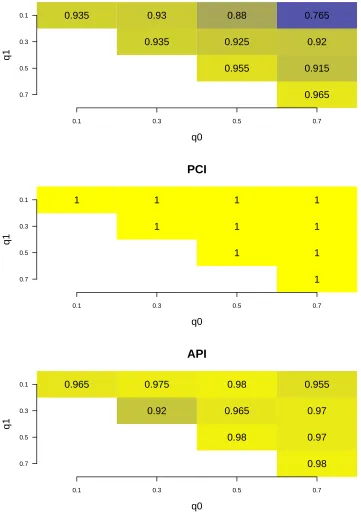
the measure related to biomarker evaluation at 95% nominal level. The texts in the plot represent the coverage rate. x-axis and y-axis are values of the two parameters q0, q1 for generated models.

Sample size n = 100, Monte Carlo replication Nrep = 200, and Bootstrap sample size B = 1000. . . 28 Figure 2.4 Monte Carlo estimates of the mean width of confidence intervals

for the measure related to biomarker evaluation at 95% nominal level. The texts in the plot represent the coverage rate. x-axis and y-axis are values of the two parametersq0, q1 for generated models.

(15)

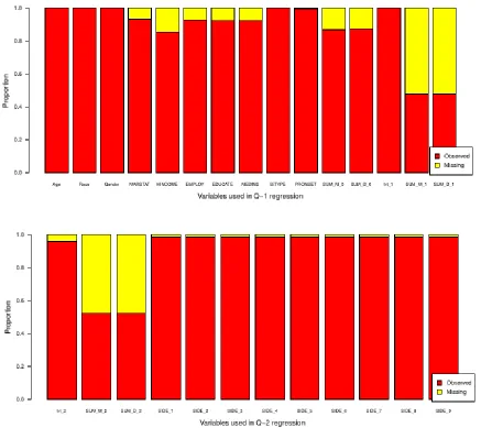
Figure 3.3 At the beginning (stage 1), there are 365 patients in total. 85 patients take Bupropion, 93 patients take Paroxetine and 187 pa-tients take placebo. After 6 weeks, 104 papa-tients’ information are lost. Only 78 patients are tracked with non-response at the end of stage 1. At stage 2, patients with non-response are assigned to secondary treatment intervention. Patients taking Bupropion or Paroxetine at stage 1 will increase current doses. But Patients taking placebo at stage 1 will be assigned Bupropion or Paroxetine. 35 Figure 3.4 Variables with missing data are listed. The SUMMi and SUMDi

denote continuous symptom subscales for depression and mood el-evation at i th stage. The Trti denotes current treatment at stage i. The responsei denotes patients’ clinical status at the end of stage i. The SIDEj represents different side effects. PRONSET denotes patients’ prior to onset clinical status. EDUCATE, EM-PLOY, MARSTAT, MEDINS and HINCOME are the indicators for patients’ education level, employment status, marriage status, medical insurance and annual home income respectively. . . 40 Figure 3.5 Estimated optimal second stage decision rule. The Q-learning

es-timated optimal second stage decision rule represented as a tree. As anticipated by the estimated second stageQ-function, SUMM1 (scale score for mood elevation) is used to dictate treatment. The tree was fit using the CART algorithm (Breiman et al., 1984) to the data {(H2i,bπ2(H2i))}i:A1i=placeboandRi=1. . . 44

Figure 3.6 Estimated optimal first stage decision rule. The Q-learning esti-mated optimal first stage decision rule represented as a tree. Note that subjects with a prior (hypo) manic episodes are recommended to receive placebo. The tree was fit using the CART algorithm (Breiman et al., 1984) to the data {H1i,bπ1(H1i)}

n

i=1. . . 46

(16)

Figure 3.8 Variables with missing data are listed. The SUMMi and SUMDi denote continuous symptom subscales for depression and mood el-evation at i th time point. The SIDEj represents different side effects. PRONSET denotes patients’ prior to onset clinical sta-tus. EDUCATE, EMPLOY, MARSTAT, MEDINS and HINCOME are the indicators for patients’ education level, employment status, marriage status, medical insurance and annual home income re-spectively. . . 55 Figure 4.1 Estimated average pain score with different thresholds. x-axis

rep-resents the different values of threshold τ for the constraint func-tion. y-axis represents the estimated efficacy score corresponding to different thresholds. . . 72 Figure 4.2 Estimated average pain score with different thresholds. y-axis

(17)

Chapter 1

Introduction

1.1

A Group of Non-smooth Estimands

Suppose we observe a dataset: D = {(Xi, Yi)}n

i=1, where Xi ∈ Rp is predictive

vari-able vector, and Yi ∈ R is the response variable. Suppose the parameter of interest is θ∗(β∗) = E{f(X, β∗)}, where f(x, β∗) is non-smooth such that (x, β∗)∈ Q(X,β∗₎.

Some-times f(x, β∗) can be rewritten asf(x, β∗) = s(x1, β1∗)·g(x2, β2∗), where x1, x2, β1∗, β

∗

2 are

subvectors of x, β∗, s(·) is continuous and differentiable, and g(·) is non-smooth when (x, β∗) ∈ Q(X,β∗₎. For example, let θ∗(β∗) = E{[XTβ∗]₊}, then f(x, β∗) = [xTβ∗]₊,

s(x1, β1∗) = xTβ

∗_{, and} _g(x

2, β2∗) = 1xT_β∗_≥₀. Here 1₍_·₎ is indicator function. Many

quan-tities of interests in history can be written in this form: the marginal mean outcome in Dynamic Treatment Regimes, regression coefficients in two-stageQ-learning, coefficients in two-stage outcome weighted learning, and measures of biomarker performance. The non-smooth functions inθ∗(β∗) can lead to non-regular asymptotics, and thus invalidate standard procedures like the bootstrap and the delta method.

The aim of this project is to construct asymptotically valid confidence intervals for this class of estimands. Berger and Boos (1994) proposed a method named projection confidence intervals (PCI) that could provide asymptotically valid CI for this group of estimands. But this method is conservative. For example, the estimated coverage rates from simulations always equal to 1.0. Based on their method, we proposed a method named adaptive projection confidence interval (API). Through this method, the PCI will only be used for points that are near the regionQ(X,β∗₎. This will reduce the conservatism

(18)

1.2

STEP-BD Study

STEP-BD (Systematic Treatment Enhancement Program for Bipolar Disorder) is a long-term study of bipolar disorder funded by the National Institute of Mental Health (NIMH). Its aim was “to generate externally valid answers to treatment effectiveness questions related to bipolar disorder” Sachs et al. (2003). Patients of age older than 15 years fulfilling DSM-IV criteria for any subtype of bipolar disorders could enter the study registry. In total, 4,360 patients from 22 sites in United States enrolled. The study lasted for 7 years (2001-2007).

Antidepressant is one kind of medication that could control the feeling of depression for patients with unipolar or bipolar disorder. But meanwhile, it may introduce some side effects for the patients. For example, it may increase of the probability of suicide for patients with bipolar disorder. Recently, some psychiatrists suggested that antidepressant may be effective for a subgroup of patients. Another common medication that is usually used for bipolar disorder patients is mood-stabilizer.

Nowadays, personalized medicine is a hot topic, and dynamic treatment regime (DTR) is one framework for personalized medicine. A DTR is a sequence of decision rules, which maps patients up-to-date information to the feasible treatments. An optimal DTR is the one that optimized the primary mean outcome across the population of interest. Historically, there are a lot of different methods that could be used to estimate the optimal DTR. These include: A-learning (Murphy 2003b),Q-learning (Watkins and Dayan 1992; Schulte et al. 2012; Laber et al. 2014c), outcome weighted learning (Zhao et al. 2012), and augmented inverse probability weighted estimator (Zhang et al. 2012a,b). Q-learning is one popular method that is easily understand and plug-in.

(19)

1.3

Constrained Sequential Dosage Assignments

When managing a chronic illness, a clinical scientist must decide how adapt treatment both in response to and anticipation of changes in each individual patient’s health status. A treatment regime formalizes this decision process as a sequence of functions, one per intervention period, that map current patient information to a recommended treatment (Murphy, 2003a; Robins, 2004; Chakraborty and Moodie, 2013). An optimal treatment regime is defined as maximizing some functional of the outcome distribution, e.g., mean symptom reduction or the probability of surviving disease-free past some time horizon, if the regime were used to select treatments for individuals in a population of interest. We consider the problem of constructing an interpretable treatment regime that adjusts treatment dosage over a potentially large number of intervention periods with the goal of maximizing a cumulative measure while controlling the risk of an adverse event. This work is motivated by a sequence of clinical trials on chronic pain in which the clinical goal was to maximize pain reduction while reducing the risk of constipation.

We use non-parametric Q-learning to form a joint estimator of the marginal mean efficacy and a general measure of risk of an adverse event for any regime in a pre-specified class. An estimator of the optimal regime is obtained by choosing the regime that maximizes expected efficacy among those that satisfy a constraint on risk. The class of regimes is chosen to ensure that the class of regimes is interepretable and easily disseminated among domain experts. We show that non-parametric Q-learning produces estimators that are more stable than (augmented) inverse probability weighting when there are a large number of time points. Furthermore, non-parametric Q-learning can be used to do diagnose severe approximation error in the class of pre-specified regimes.

1.4

Outline

The outline of the thesis is as follows:

(20)

In Chapter 3, we focused on data analysis of STEP-BD. Section 3.1 introduce the STEP-BD study. In Section 3.2, we analysis the data set from RAD (Randomized Acute Depression Pathway) using Q-learning. In Section 3.3, we analysis the data set named SAD (Standardized Acute Depression) using the method of grouped Q-learning.

(21)

Chapter 2

Adaptive Projection Confidence

Interval for Non-smooth Estimands

2.1

Introduction

Consider a regression problem in which we observe a dataset, D = {(Xi, Yi)}ni=1, where

Xi ∈ Rp denotes predictive variables, and Yi ∈ R is the response variable. Suppose we are interested in an estimand, say θ∗(β∗) = E{f(X, β∗)}, where β∗ is a nuisance parameter,f(·) is a known function, andXis a random vector with the same distribution as predictor Xi. Suppose the function f(x, β∗) is non-smooth in the region denoted as

Q(X,β∗₎, where we assume Q₍_X,β∗₎ is a closed set. The term non-smooth here means

that f(x, β∗) is not differentiable at any point (x, β∗) ∈ Q(X,β∗₎. We assume f(x, β∗) is

continuous and differentiable for all (x, β∗)∈ Q/ (X,β∗₎. For example, if our target estimand

is θ∗(β∗) = E{[XT_β∗_]

+}, where f(x, β∗) = [xTβ∗]+. The non-smooth region Q(X,β∗₎ for

this example is {(x, β∗) : xT_β∗ _{= 0}_}_. _{In many cases, the function} _f_{(x, β}∗_{) can be}

rewritten as the multiplication of two functions: a smooth functions(x1, β1∗) and a

non-smooth function g(x2, β2∗), whereg(·) is an indicator function, andβ

∗

1 and β

∗

2 are subsets

ofβ∗that can have same elements. For the example above, the correspondings(·) andg(·) will be s(x1, β1∗) =xTβ∗, and g(x2, β2∗) = 1xT_β∗_≥₀, where x₁ =x₂ =x and β₁∗ =β₂∗ =β∗.

(22)

2014). In this chapter, we focus on the construction of a confidence interval (CI) for the non-smooth estimands of the form θ∗(β∗)_,E{s(X1, β1∗)g(X2, β2∗)}.

For estimand θ∗(β∗), let ˆβn denote an estimator based on the dataset D. A natural estimator of θ∗(β∗) is ˆθn( ˆβn) = En{f(X,βˆn)} = En{s(X1,βˆ1n)g(X2,βˆ2n)}, where En represents empirical expectation, i.e.,Enh(X) = 1_nPn

i=1h(Xi). We assume that

√

n( ˆβn− β∗) is asymptotically normally distributed with mean 0 and positive definite variance matrix denoted as Ωβ∗. If P{(x, β∗)∈ Q₍_X,β∗₎}= 0, then the asymptotic distribution of

√

n{θˆn( ˆβn)−θ∗(β∗)} can be derived using the delta method. Hence, an asymptotically valid CI can be constructed using this limiting distribution. However, if P{(x, β∗) ∈ Q(X,β∗₎}>0, then the limiting distribution of

√

n{θn( ˆˆ βn)−θ∗(β∗)}may depend abruptly on the value of β∗ and the distribution of X. Therefore, standard methods such as asymptotic approximations or the delta method cannot be applied.

(23)

regimes (DTR) (Chakraborty et al., 2014). Thism-out-of-n method can provide valid CI in both regular and nonregular situations. Laber et al. (2014c) proposed the Adaptive Confidence Interval (ACI) for the first stage coefficients in Q-learning. They created smooth upper and lower bounds on the non-smooth estimand, and use them to construct confidence intervals. But it is difficult to compute these bounds and to generalize them to new settings. Thus, it is difficult to apply ACI to other estimands.

Based on the PCI, we propose an adaptive method to construct an asymptotically valid CI. We call it Adaptive Projection Interval (API). The API can be used with es-timands on the form θ∗(β∗) = E{s(X1, β1∗)g(X2, β2∗)} discussed previously. When using

the API, standard methods such as the percentile bootstrap will be applied to observa-tions that are not in the region Q(X,β∗₎, while PCI will be applied to observations that

are in the region Q(X,β∗₎. Therefore the API will gain the benefit from both percentile

bootstrap and PCI. We prove that it provides an asymptotically valid CI for both regular and nonregular situations. The outline of this chapter is as follows. Section 2.2 reviews existing methods for constructing a valid CI for non-smooth estimands. The construction and tuning of the API and its theoretical properties are illustrated in Section 2.3. Section 2.4 presents a numerical study of the API. Section 2.5 concludes the chapter. Proofs of theoretical results are referred to an appendix.

2.2

Review of Existing methods

In this section, we review the following methods for constructing confidence intervals for non-smooth estimands: the percentile bootstrap confidence interval (CPB), the projec-tion confidence interval (PCI), them-out-of-nsubsampling bootstrap confidence interval (MOFN), and the adaptive confidence interval (ACI).

2.2.1

Percentile Bootstrap Confidence Interval

The percentile bootstrap method was first proposed by Efron (1979). A (1−2α)×100% percentile bootstrap CI for θ∗(β∗) is constructed as follows.

Step 1 For b= 1,2, ..., B,

• drawn observations with replacement from D, denote the sampled data D(b)_;

(24)

Step 2 Take the empiricalα×100 and (1−α)×100 percentiles of bootstrap estimators ˆ

θn(1)( ˆβn(1)),θˆn(2)( ˆβn(2)), ...,θˆ(nB)( ˆβn(B)). These two empirical percentiles will construct the (1−2α)×100% bootstrap percentile CI for θ∗(β∗).

If we use ˆKB denote the empirical distribution function of these bootstrap values, then the (1−2α)×100% percentile bootstrap confidence interval is :

ˆ

K_B−1(α),Kˆ_B−1(1−α).

When f(x, β∗) is continuous, or β∗ is a fixed and known, then under mild regularity condition, the CPB provides an asymptotically valid CI. However, in our situation, β∗ is a parameter that is unknown, and f(x, β∗) is not differentiable in the region Q(X,β∗₎.

Therefore, the CI constructed by percentile bootstrapping through estimator ˆθn( ˆβn) may not provide nominal coverage.

2.2.2

Projection Confidence Interval

The projection confidence interval (PCI) was first introduced by Berger and Boos (1994). Later it was discussed by Robins (2004). A projection region for the target parameter θ∗(β∗) is constructed as follows. First, construct a (1− η)× 100% confidence region for β∗, say C(1−η),β∗. Second, for each β ∈ C₍₁₋_η₎_,β∗, a central bootstrap confidence

interval I(1−α),θ∗₍_β₎ for the corresponding estimand θ∗(β) = E{f(X, β)} can be formed

through the limiting distribution of √n{θˆn(β) −θ∗(β)}, where ˆθn(β) = En{f(X, β)}. The projection confidence region forθ∗(β∗) is defined as the union of I(1−α),θ∗₍_β₎ over all

β ∈ C(1−η),β∗, which is denoted asU₍₁₋_α₋_η₎_,θ∗. There are two chances to have mistake with

this approach: (i)β∗ may be not belong to C(1−η),β∗, and this will occur with probability

no more than η; (ii)β∗ ∈ C(1−η),β∗ but θ∗(β∗) may not belong toI₍₁₋_α₎_,θ∗₍_β₎, and this will

occur with probability no more than α. Thus the probability that θ∗(β∗) ∈ U/ (1−α−η),θ∗

satisfies:

Pr{θ∗(β∗)∈ U/ (1−α−η),θ∗} = Pr{θ∗(β∗)∈ U/ ₍₁₋_α₋_η₎_,θ∗, β∗ ∈ C₍₁₋_η₎_,β∗}+

Pr{θ∗(β∗)∈ U/ (1−α−η),θ∗, β∗ ∈ C/ ₍₁₋_η₎_,β∗}

≤ Pr{θ∗(β∗)∈ I/ (1−α),θ∗₍_β∗₎}+ Pr{β∗ ∈ C/ ₍₁₋_η₎_,β∗}

(25)

This means the probability that θ∗(β∗) ∈ U/ (1−α−η),θ∗ is less or equal to α+η, which

satisfies the definition of validity for confidence interval. Hence, the coverage rate of the projection confidence region is at least (1−α−η)×100%.

In our model set up, the PCI is implemented as follows. Let ˆβn denote an consistent estimator ofβ∗ such that √n( ˆβn−β∗) converges in distribution to N(0,Ωβ∗), where Ω_β∗

is positive semi-definite. Let ˆΩ_βˆ_n denote a consistent estimator of Ωβ∗, which is smooth

in a neighbor of β∗. A wald-type asymptotic (1−η)×100% confidence region for β∗ is therefore

C(1−η),β∗ ,

n

β∈Rdim(β∗) _:_{n( ˆ}_β

n−β)TΩˆ_βˆ_n( ˆβn−β)≤χ21−η,dim(β∗₎

o

,

whereχ2

1−η,d is the (1−η)×100 percentile of aχ2-distribution withddegrees of freedom. And for eachβ ∈ C(1−η),β∗fixed, it follows from standard argument that

√

n(ˆθn(β)−θ∗(β)) is regular, asymptotically normal with mean zero, where ˆθn(β) =En{f(X, β)}. This is because for β fixed and assuming Var{f(X, β)} exists, the central limit theorem can be applied to √n(ˆθn(β)−θ∗(β)). Thus, standard methods for constructing confidence interval, e.g. the percentile bootstrap, can be used to form a valid (1 − α)× 100% confidence interval for θ∗(β), say I(1−α),θ∗₍_β₎. Then, the union

U(1−α−η),θ∗ =

[

β∈C₍₁−η),β∗

I(1−α),θ∗₍_β₎, (2.1)

is a (1−α−η)×100% projection confidence interval (PCI) for θ∗(β∗).

The PCI is appealing because it is conceptually simple. However, it may be conser-vative especially when P{(x, β∗)∈ Q(X,β∗₎}= 0. For example, let θ∗(β∗) = E([XTβ∗]₊),

where the parameterβ∗ is from multiple linear regression model. We know that [xT_β∗_]

+

is non-smooth when (x, β∗) ∈ {(x, β∗) : xT_β∗ _{= 0}_}_{. Suppose P}_{_XT_β∗ _> ₀_} _{= 1. Then}

the estimand can be rewritten as E(XT_β∗_{) = E(X)}T_β∗_{. Thus, standard methods, e.g.,}

(26)

2.2.3

m

-out-of-

n

Subsampling Bootstrap Confidence Interval

Them-out-of-nbootstrap is one possible approach to produce valid confidence interval for non-smooth estimands (Bretagnolle 1983; Swanepoel 1986; Shao and Wu 1989; D¨umbgen 1993; Shao 1994; Huang et al. 1996; Bickel et al. 1997). Instead of resampling bootstrap samples of size n, the m-out-of-n bootstrap draws bootstrap samples of size m, which is a smaller order than the original sample size n. This means m depends on n, tends to infinity, and satisfies m

n → 0 (or we say, m = o(n)). A (1−2α)×100% m-out-of-n bootstrap CI for θ∗(β∗) is constructed as follows:

Step 1 For m= 1,2, ..., B,

• drawm observations with replacement fromD, denote the sampled data D(mb);

• construct the corresponding estimator ˆθm(b)( ˆβm(b)) for θ∗(β∗) using D(mb).

Step 2 Take the empiricalα×100 and (1−α)×100 percentiles of bootstrap estimators ˆ

θm(1)( ˆβm(1)),θˆm(2)( ˆβm(2)), ...,θˆ(mB)( ˆβm(B)). These two empirical percentiles will construct the (1−2α)×100% m-out-of-n bootstrap CI for θ∗(β∗).

One difficulty associated with this method is the choice of m in finite sample. Since the condition m =o(n) is asymptotic, and thus no guidance is provided for finite sam-ples. Intuitively, the choice of the resample size m should reflect the non-regularity of the estimand. Using the idea from Bickel and Sakov (2008), Chakraborty et al. (2013b) proposed a data adaptive choice of m based on a measure of non-regularity. They ap-plied their method to construct CIs for coefficients in Q-learning. Chakraborty et al. (2013b) consider a class of resample sizes of the form m _, nf(p), where f(p) satisfies: (i) f(p) is monotone decreasing in p, where p ∈ (0,1], and f(0) = 1; and (ii) f(p) is continuous and its first derivative is bounded. A plug-in estimator of p is defined as ˆ

p = En1_{_Tˆ_n₍_X,_βˆ_n₎≤τn}, where ˆTn(X,

ˆ

βn) is a test statistic testing H0 : (x, β∗) ∈ QX,β∗,

reject the test if ˆTn(x,βˆn) > τn, and τn is a potential tuning parameter. They used f(p) = 1+ν₁₊(1_ν−p), but other choices of f(p) are possible. The corresponding estimator of m is then defined as:

ˆ

m=n1+ν(11+ν−p)ˆ ,

(27)

mean outcome in dynamic treatment regimes (DTRs). The expression for estimator ˆm is similar. It can be shown that m-out-of-n subsampling confidence interval forming in this way is asymptotically valid.

2.2.4

Adaptive Confidence Interval (ACI)

Similar to the adaptive confidence interval for misclassification rate (Laber and Murphy, 2011), Laber et al. (2014c) proposed an adaptive confidence interval (ACI) to construct an asymptotically valid confidence interval for linear combinations of the first stage co-efficients in Q-learning. Letθ∗(β∗) denote the multiplication of the first stage coefficient vector, and let ˆθn( ˆβn) denote the estimator of θ∗(β∗). Because of non-regularity, it is impossible to construct a uniformly convergent estimator of the limiting distribution of

√

n{θn( ˆˆ βn)−θ∗(β∗)} (Van Der Vaart, 1991; Hirano and Porter, 2012). Instead of con-structing a CI for θ∗(β∗) directly, Laber et al. (2014c) construct an upper bound and a lower bound for √n{θˆn( ˆβn)−θ∗(β∗)}. These two bounds can be regular and uniformly convergent. Thus a confidence interval for θ∗(β∗) can be formed by bootstrapping these two bounds.

To limit the conservatism, these bounds are defined only based on the non-smooth term g(X2, β2∗) of the target estimand θ∗(β∗) = E{s(X1, β1∗)g(X2, β2∗)}, and only applied

to subjects in the non-smooth regionQ(X,β∗₎. To achieve this, a “pretest” (Olshen, 1973;

Andrews, 2001; Cheng, 2008; Andrews and Guggenberger, 2009) is used to partition the observed data into two groups: (Group 1) observations that are not in the non-smooth region; and (Group 2) observations that are near in the non-non-smooth region. A test statistic ˆTn(x,βˆn) is used to achieve the partition: assign a subject to Group 1 if ˆTn(x,βˆn) > λn and Group 2 otherwise. The λn is a tuning parameter that can be estimated using double bootstrapping.

Let U denote the upper bound, and let L denote the lower bound of √n{θˆn( ˆβn)− θ∗(β∗)} proposed in this procedure. Noting that

ˆ

θn( ˆβn)− U/

√

n ≤θ∗(β∗)≤θˆn( ˆβn)− L/

√

n,

(28)

interval (ACI) forθ∗(β∗) is defined:

ˆ

θn( ˆβn)−u/ˆ √n,θn( ˆˆ βn)−ˆl/√n

.

The ACI can provide a asymptotically valid confidence interval for non-regular estimand. But its construction of the upper and lower bounds may be too complicated.

2.3

Adaptive Projection Interval

In this section, we propose the adaptive projection interval, which is a asymptotically valid confidence interval for the estimands we have defined before. We first introduce the construction of API. We then discuss the algorithm of tuning the parameter in API.

2.3.1

Construction of API

We propose a method of constructing a confidence interval that is consistent in non-regular framework. We refer to this method as the Adaptive Projection Interval (API). The API is inspired on the idea of projection confidence interval (PCI), which is pro-posed by Robins (2004). The details for PCI is introduced in 2.2.2. Note that the estimand of interest has the term: θ∗(β∗) = E{s(X1, β1∗)g(X2, β2∗)}, where s(·)

rep-resents smooth part and g(·) represents non-smooth part (e.g. indicator function) in a region Q(X,β∗₎. Let ˆβ_n denote a consistent estimator for β∗. And define estimator

ˆ

θn( ˆβn) = En{s(X1,βˆ1n)g(X2,βˆ2n)}. Recall that generally it is impossible to construct a uniformly convergent estimator of the limiting distribution of √n(ˆθn( ˆβn)−θ∗(β∗)). Pro-jection confidence interval is one possible approach to construct confidence interval for θ∗(β∗). But it may be too conservative. Our approach is applying the idea of projection confidence interval to an adaptive estimator for θ∗(β∗).

First, note that the observed dataset D can be partitioned into two groups: (Group 1) points that are not in the non-smooth region Q(X,β∗₎; and (Group 2) points that are

(29)

be decomposed as: ˆ

θn( ˆβn) = En{s(X1,βˆ1n)g(X2,βˆ2n)}

= En{s(X1,βˆ1n)g(X2,βˆ2n)1(X,β∗₎_∈Q_/

(X,β∗)}

+En{s(X1,βˆ1n)g(X2,βˆ2n)1(X,β∗₎_∈Q

(X,β∗)},

where 1· is the indicator function. The first term on the right-hand side corresponds to

points that are not in the non-smooth region (Group 1), and the second term corresponds to points that are in the non-smooth region (Group 2). Similarly, the estimand θ∗(β∗) can also be written in this style:

θ∗(β∗) = E{s(X1, β1∗)g(X2, β2∗)}

= E{s(X1, β1∗)g(X2, β2∗)1(X,β∗₎_∈Q_/

(X,β∗)}

+E{s(X1, β1∗)g(X2, β2∗)1(X,β∗₎_∈Q

(X,β∗)}.

Sinceβ∗ is unknown, to achieve the partition, we use a “pretest” (Olshen, 1973; Andrews, 2001; Cheng, 2008; Andrews and Guggenberger, 2009; Andrews and Soares, 2010). The pretest is based on ˆTn(X,βˆn), which is a test statistic that diverges to +∞when (x, β∗)∈/

Q(X,β∗₎ but is bounded in probability when (x, β∗) ∈ Q₍_X,β∗₎. For each X = x, this

test statistic testing: H0 : (x, β∗) ∈ Q(X,β∗₎ against the alternative. Reject the test if

ˆ

Tn(x,βˆn)> λn, whereλn is a potential tuning parameter. Then using the pretest, ˆθn( ˆβn) can be rewritten as:

ˆ

θn( ˆβn) = En{s(X1,βˆ1n)g(X2,βˆ2n)1_Tˆ_n₍_X,_βˆ_n₎_>λ_n}

+En{s(X1,βˆ1n)g(X2,βˆ2n)1_Tˆ_n₍_X,_βˆ_n₎_≤_λ_n}.

Let C(1−η),β∗ denote the (1 −η)× 100% confidence region for nuisance parameter β∗

from limiting distribution of √n( ˆβn−β∗). In projection confidence interval, for each β ∈ C(1−η),β∗, a confidence interval is constructed based on the limiting distribution of

√

n{θˆn(β)−θ∗(β)}. But in adaptive projection interval, we consider an adaptive estimator ˆ

θn(β,βˆn):

ˆ

θn(β,βˆn) = En{s(X1,βˆ1n)g(X2,βˆ2n)1Tn(X,βˆn)>λn}

(30)

where β2 is the corresponding subset ofβ. We also define the estimand θ∗(β, β∗):

θ∗(β, β∗) = E{s(X1, β1∗)g(X2, β2∗)1(X,β∗₎_∈Q_/

(X,β∗)}

+E{s(X1, β1∗)g(X2, β2)1(X,β∗₎_∈Q

(X,β∗)}. (2.3)

It can be shown that √n{θˆn(β,βˆn) − θ∗(β, β∗)} is asymptotically normal with finite variance (details see in Section A.1). Hence for each β ∈ C(1−η),β∗, a (1−α)×100%

confidence interval based on this limiting distribution can be constructed using non-parametric bootstrapping. We denote this confidence interval asI(1−α),θ∗₍_β,β∗₎. Then the

union:

e

U(1−α−η),θ∗₍_β∗₎ =

[

β∈C₍₁−η),β∗

I(1−α),θ∗₍_β,β∗₎ (2.4)

is a (1−α−η)×100% adaptive projection interval (API) forθ∗(β∗). The API is adaptive in two ways. First, it provides an asymptotically valid confidence interval regardless of the non-smoothness. Specifically, this is achieved by applying PCI to points that are in the region Q(X,β∗₎ through a test statistic. Secondly, it restricts the scale of non-smooth

part. Because instead of usingf(X, β) = s(X1, β1)g(X2, β2) to construct the PCI, it uses

f(X, β,βˆn) = s(X1,βˆn)g(X2, β2) to form the PCI.

2.3.2

Choice of Tuning Parameter

In the construction of adaptive projection interval (API), it is important to decide the value of tuning parameter λn. Recall that

√

n( ˆβn−β∗) is asymptotic normal with mean 0 and variance matrix Ωβ∗. Then the test statistic ˆTn(x,βn) can beˆ n(x

T_βˆ_n₎2

xT_Ωˆ_β∗x , where ˆΩβ∗ is a plug-in estimator for Ωβ∗. Then a potential cutting value can be defined asχ2

1−α,dim(β∗₎,

which is the (1−α)×100 percentile of aχ2_{-distribution with dim(β}∗_{) degrees of freedom.}

We then consider a range of values ofλnof the formλn=τ χ2₁−α,dim(β∗₎, whereτ ∈[m, M]

with 0< m < M <+∞. A double bootstrap procedure (see Davison and Hinkley 1997 for details) is used here for choosing the tuning parameter λn (or τ) in a data-driven manner. This procedure appears to reduce conservatism in simulations.

Consider a grid of candidate values for τ; for example, {0.025,0.05,0.075, ...,1}. The algorithm is as follows:

(31)

• Draw B1 bootstrap samples from the data D. For each bootstrap sample data

D(b1)_,_b

1 = 1, ..., B1, and for each τi ∈ {0.025,0.05,0.075, ...,1} do the following:

1. calculate the corresponding confidence region of β∗, C(b1)

(1−η),β∗, based on the

limiting distribution of √n( ˆβ(b1)

n −β∗). 2. Conditional on sample D(b1)_{, draw} _B

2 bootstrap samples: D(b1,1), ...,D(b1,B2).

3. For each double bootstrap sample D(b1,b2)_, _b

2 = 1, ..., B2, and each point β ∈

C(b1)

(1−η),β∗, compute the adaptive estimator ˆθn(β,βˆ

(b1,b2)

n ) with tuning parameter λn=τiχ2₁₋_α,_dim(_β∗₎.

4. For each fixed β, calculate the non-parametric bootstrap (1−α)×100% con-fidence intervalI(b1)

(1−α),θ∗₍_β,β∗₎ for θ∗(β, β∗) based on these ˆθn(β,βˆ

(b1,b2)

n ). 5. Take unions ofI(b1)

(1−α),θ∗₍_β,β∗₎for all β ∈ C

(b1)

(1−η),β∗ to get the adaptive confidence

intervalUe

(b1)

(1−α−η),θ∗₍_β∗₎.

• Estimate the coverage rate of the double bootstrap CIs Ue

(b1)

(1−α−η),θ∗₍_β∗₎ from

first-stage bootstrap data D(b1) _{for each} _τi

1 B1

B1

X

b1=1

1_θ_ˆ

n( ˆβn)∈Ue (b₁₎

(1−α−η),θ∗(β∗)

.

• Pick the value of τi that has the coverage rate nearest to the significant level (1−α−η).

2.4

Empirical Study

One main advantage of the API is that it provides valid coverage rate for the estimand with expression θ∗(β∗) = E{s(X1, β1∗)g(X2, β2∗)} under both smooth and non-smooth

(32)

the performance of API for inference of multi-stageQ-learning. The forth example shows the performance of API for the estimand related to biomarker evaluation. In general, we consider the construction of 95% confidence intervals for these four examples. We compare the empirical performance of the API with the following methods: the centered percentile bootstrap (CPB) as described in Section 2.2.1; the projection confidence in-terval (PCI) as described in Section 2.2.2 with parameter fixed atη = 0.01, α = 0.05; the adaptive m-out-of-n (MOFN) bootstrap with data-drive tuning as described in Section 2.2.3.

2.4.1

Toy Example

The target estimand for this example is θ∗(β∗) = E[XTβ∗]+. The non-smooth region of

(X, β∗) for this example satisfying: XTβ∗ = 0. Five generative models are used in these evaluations. Each of the models are generated from:

• X ∼Np(0,AR(0.5))

• β∗ = (√i

np, ..., i

√

np) T p

• Y =XT_β∗₊_, _∼_N(0,₁₎

where X and are independent, and variance matrix AR(d) is a symmetric matrix with value d|i−j| for the ith row the jth column element. Sample size is fixed at n = 20; dimension of β∗ is also fixed at p = 3; and i has values: 0.5, 1, 2, 3, 4. As i increases, θ∗(β∗) will be far away from the non-smooth point 0.

Table 2.1 shows the coverage probabilities of the simulations. Table 2.2 shows the mean width of confidence intervals. As expected, CIs constructed via the CPB method have the smallest average width; however, these are associated with under-coverage under non-regular situation. On the other hand, PCI method always gives the widest CIs, with coverage rates often over the nominal level. Our proposed API method with data-driven λn always offers valid coverage rates. By fine-tuning λn, it reduce the conservatism in regular cases.

(33)

Table 2.1: Monte Carlo estimates of coverage probabilities of confidence intervals for the toy example at 95% nominal level. The rows represent different methods of constructing CIs: (i) then-out-of-ncentered percentile bootstrap (CPB); (ii) the projection confidence interval (PCI); (iii) the proposed adaptive projection interval (API). Estimates are con-structed using 200 datasets, and 500 bootstraps drawn from each dataset. Coverage rate significantly different from 0.95 at the 0.05 level are in bold. The ones that significantly below 0.95 are marked with ∗.

Toy Example i= 0.5 i= 1 i= 2 i= 3 i= 4 CPB 0.88∗ 0.93 0.93 0.94 0.94

PCI 1.0 0.98 0.98 0.99 1.0

API 0.93 0.93 0.95 0.93 0.96

Table 2.2: Monte Carlo estimates of the mean width of confidence intervals for the toy example at 95% nominal level. The rows represent different methods of constructing CIs: (i) the n-out-of-n centered percentile bootstrap (CPB); (ii) the projection confi-dence interval (PCI); (iii) the proposed adaptive projection interval (API). estimates are constructed using 200 datasets, and 500 bootstraps from each dataset. Widths with cov-erage rate significantly different from 0.95 at the 0.05 level are in bold. The ones with coverage rate significantly below 0.95 are marked with ∗.

Toy Example i= 0.5 i= 1 i= 2 i= 3 i= 4 CPB 0.49∗ 0.56 0.67 0.73 0.85

(34)

et al., 2007; Zhao et al., 2011), HIV infection (Khalili and Armaou, 2008; Robins et al., 2008), and mental illnesses (Dawson and Lavori, 2004; Shortreed and Moodie, 2012). A dynamic treatment regime (DTR) is a sequence of decision rules, one per stage, which dictates individualized treatment assignment evolving patients’ up-to-date information. These regimes can be widely used for chronic illness. Usually, we use V alue to evaluate the quality of a DTR. The V alue of a DTR is the average primary outcome obtained when the DTR is applied to the entire population of interest. We say a DTR is optimal if its correspondingV alue is highest.

Here, we focus on one-stage DTR. Define data D = {(Xi, Ai, Yi) : i = 1, ..., n;Xi ∈

Rp_;_Yi _∈_R_;_Ai _{∈ {−}_1,₁_}} _where: _Xi _{is the} _{ith subject information,} _Yi ₌_{r(Xi, Ai) is the} continuous outcome forith subject with a known functionr(·), andAi denotes treatment assigned for theith subject. The outcomeYiis the larger the better. We define treatment regime π as a map: Rp _{→ {−}_1,₁_} _{such that patient with information} _X ₌_x _{is assigned} to treatment π(x). Then for a fixed DTR π, its V alue is

Vπ = Eπ[Y] = Eπ[r(X, A)],

where Eπ denotes expectation with respect to the distribution of entire data. Usually for a feasible regime π, one can use inverse probability weighting (IPW) to express the V alueof the regime in terms of the generative model (Robins et al., 2000; Murphy et al., 2001). This IPW estimator is

Vπ = Eπ[Y] = Eπ

₁

π(X)=A Pr(A|X)Y

, (2.5)

where 1(·) is indicator function, and Pr(A|X) is the treatment allocation probability.

Then a plug-in estimator for Vπ _{will be:} ˆ

Vπ =En

1π(X)=A Pr(A|X)Y

, (2.6)

where En denotes the empirical expectation. From (2.5), we know that the V alue of a DTR is non-regular because of the indicator function.

(35)

Each of the models are generated from:

• X =W1u≥ρ+E⊥β∗W1_u<ρ

• W ∼Np(0, Ip), P⊥β∗W =W − hW,β∗i hβ∗_,β∗_iβ

∗T

• A∈ {−1,1}, A∼Bernoulli(0.5)

• Y =XT_ψ∗₊_AXT_β∗₊_e, _e_∼_N(0,₁₎

where parameter u is uniform distributed in (0,1), and ρ is a runing parameter taking values {0.1,0.4,0.7,0.9}. We fix ψ∗ = 1p, and define β∗ = c1p, where c is a tuning parameter taking values {0.1,0.4,0.7,0.9}. We also fix dimension p= 10.

Figure 2.1 shows the estimated coverage rate for different methods: CPB (central percentile bootstrap), PCI (projection confidence interval), MOFN (m-out-of-n adaptive bootstrap), and API (adaptive projection interval). Figure 2.2 shows the corresponding average width for these confidence intervals. CIs constructed via CPB method have the smallest average width; however, under non-regular situations CPB often under-coverage. On the contrast, CIs formed by PCI method always have the largest average width, but with coverage rate often significantly above the 95% nominal level. It is surprising that in some non-regular cases, coverage rates from confidence intervals constructed by MOFN are significantly lower than the 95% nominal level. But our proposed method, API, always have coverage rates around the 95% nominal level, with considerable average CI width.

2.4.3

Q

-learning First Stage Covariates

In section 2.4.2, we mentioned the idea of dynamic treatment regime (DTR). An optimal dynamic treatment regime is the DTR that optimizes the expectation of a cumulative outcome over a population of interest. Recently, there are numerous methods proposed to estimate the optimal DTR. These includeQ-learning (Murphy, 2005a; Chakraborty and Moodie, 2013; Laber et al., 2014a), A-learning (Murphy, 2003a; Robins, 2004), outcome weighted learning (Zhao et al., 2012, 2014), and augmented value maximization (Zhang et al., 2012b, 2013). Among these methods, Q-learning is one of the most important one. So in this subsection, we discuss the simulation results from Q-learning.

We consider two stage two treatment Q-learning. The observed data set is defined as

(36)

CPB

rho

c

0.1 0.4 0.7 0.9

0.9 0.7 0.4

0.1 0.92 0.96 0.86 0.7

0.96 0.94 0.84 0.71

0.93 0.9 0.88 0.79

0.95 0.89 0.93 0.77

PCI

rho

c

0.1 0.4 0.7 0.9

0.9 0.7 0.4

0.1 1 1 1 1

0.99 1 1 1

0.98 1 1 1

0.98 0.97 0.99 1

MOFN

rho

c

0.1 0.4 0.7 0.9

0.9 0.7 0.4

0.1 0.95 0.97 0.91 0.8

0.98 0.98 0.87 0.77

0.95 0.93 0.89 0.87

0.96 0.93 0.93 0.82

API

rho

c

0.1 0.4 0.7 0.9

0.9 0.7 0.4

0.1 0.99 0.99 0.99 0.95

0.97 0.97 0.92 0.91

0.93 0.94 0.93 0.95

0.95 0.94 0.94 0.93

(37)

CPB

rho

c

0.1 0.4 0.7 0.9

0.9 0.7 0.4

0.1 1.546 1.288 1.02 0.735

1.479 1.275 0.964 0.719

1.618 1.389 1.048 0.756

1.752 1.463 1.1 0.754

PCI

rho

c

0.1 0.4 0.7 0.9

0.9 0.7 0.4

0.1 2.83 2.36 1.912 1.379

2.059 1.851 1.522 1.27

2.034 1.873 1.559 1.258

2.149 1.934 1.61 1.262

MOFN

rho

c

0.1 0.4 0.7 0.9

0.9 0.7 0.4

0.1 1.668 1.395 1.165 0.898

1.58 1.363 1.029 0.827

1.7 1.503 1.156 0.855

1.803 1.572 1.181 0.859

API

rho

c

0.1 0.4 0.7 0.9

0.9 0.7 0.4

0.1 1.888 1.593 1.276 0.945

1.648 1.447 1.123 0.894

1.757 1.558 1.211 0.915

1.896 1.624 1.259 0.916

(38)

subject information; A1 ∈ A1 denotes the first stage treatment assignment; X2 ∈ Rp2

denotes information collected during the course of the first stage treatment including information dictating first-stage responder status; A2 ∈ A2 denotes the second stage

treatment assignment; andY ∈R denotes a continuous outcome measured at the end of the study coded so that larger values are better. Let Ht,t = 1,2 denote the information collected before time t. Then H1 = X1, and H2 = (X1T, A1, X2T). Also, we define

At ∈ {−1,1} The optimal DTR, πopt, is the one satisfying Eπ

opt

Y = sup_πEπY. In two-stage setting, a DTR is defined as a pair of decision rules π = (π1, π2), where πt : dom(Ht) → dom(At). The optimal DTR can be characterized by Q-functions. In the two-stage setting, we define theQ-functions as (Sutton and Barto, 1998; Murphy, 2005a)

Q2(h2, a2) , E(Y|H2 =h2, A2 =a2),

Q1(h1, a1) , E{maxa2Q2(H2, a2)|H1 =h1, A1 =a1}.

In this setting, the optimal DTR can be calculated by dynamic programming (Bellman, 1957), and the solution is π_tdp(ht) = argmaxatQt(ht, at).

Q-learning estimates the optimal DTR by plug-in regression models for theQ-functions. Usually, we consider linear regression models, which have the form Qt(ht, at;βt) = hT_t,₀βt,0 +athTt,1βt,1, ht,0 and ht,1 are known sub vectors of ht and βt = (βt,T0, βt,T1)T. Then

byQ-learning algorithm, the estimated coefficients from stage 1 regression is : ˆ

β1 = arg minβ1En

˜

Y −Q1(H1, A1;β1)

2

,

where ˜Y represents the predicted second stage outcome: ˜Y = maxa2Q2(H2, a2; ˆβ2) with

ˆ

β2 = arg minβ2En(Y −Q2(H2, A2;β2))

2

. We then define the following population analogs of the estimators in Q-learning:

β₁∗ = arg min_β₁E

˜

Y∗−Q1(H1, A1;β1)

2

,

where ˜Y∗ = maxa2Q2(H2, a2;β

∗

2) =H2T,0β

∗

2,0+|H2T,1β

∗

2,1|, andβ

∗

2 = arg minβ2E (Y −Q2(H2, A2;β2))

2

. Our target here is to construct 95% confidence interval for cT_β∗

1, where c is a constant

(39)

Table 2.3: Parameters indexing the example models. Examples are designated NR=nonregular, NNR=near-nonregular, R=regular.

EX. γ δ Type Regularity Measures

1 (0,0,0,0,0,0,0)T _(0.5,_0.5)T _NR _p_{= 1} _φ _{= 0/0} 2 (0,0,0,0,0.01,0,0)T _(0.5,_0.5)T _NNR _p_{= 0} _φ₌_∞ 3 (0,0,−0.5,0,0.5,0,0.5)T (0.5,0.5)T NR p= 1/2 φ = 1.0 4 (0,0,−0.5,0,0.5,0,0.49)T _(0.5,_0.5)T _NNR _p_{= 0} _φ_{= 1.02} 5 (0,0,−0.5,0,1.0,0.5,0.5)T _(1.0,_0.0)T _NR _p_{= 1/4} _φ_{= 1.41} 6 (0,0,−0.5,0,0.25,0.5,0.5)T (0.1,0.1)T R p= 0 φ= 0.35 A (0,0,−0.25,0,0.75,0.5,0.5)T _(0.1,_0.1)T _R _p_{= 0} _φ_{= 1.035} B (0,0,0,0,0.25,0,0.25)T (0,0)T NR p= 1/2 φ= 1.00 C (0,0,0,0,0.25,0,0.24)T _(0,₀₎T _NNR _p_{= 0} _φ_{= 1.03}

(MOFN) bootstrap with data-driven tuning (Chakraborty et al., 2013a). Nine genera-tive models are used in these evaluations (Chakraborty et al., 2009). Each of the models can be expressed as:

• Xt ∈ {−1,1}, At∈ {−1,1}for t∈ {1,2}

• P(A1 = 1) =P(A1 =−1) = 0.5,P(A2 = 1) =P(A2 =−1) = 0.5

• X1 ∼Bernoulli(0.5), X2|X1, A1 ∼Bernoulli(expit(δ1X1+δ2A1))

• Y2 =γ1+γ2X1+γ3A1+γ4X1A1+γ5A2+γ6X2A2+γ7A1A2 +, ∼N(0,1)

where expit(x) =ex_{/(1 +}_ex_{). The nine generative models are generated by different} _{δ, γ} combinations. Table 2.3 shows the information of nine generative models. The patients’ history is defined as

H2,0 = (1, X1, A1, X1A1, X2)T, H2,1 = (1, X2, A1)T,

H1,0 = (1, X1)T, H1,1 = (1, X1)T.

Then the simulation models are given by Q2(H2, A2;β2) = H2T,0β2,0 +H2T,1β2,1A2, and

Q1(H1, A1;β1) = H1T,0β1,0 +H1T,1β1,1A1. The regularity is defined as p = P(γ5A2 +

γ6X2A2+γ7A1A2 = 0); and the standardized effect size is defined as φ= E[γ5+γ6X2+

γ7A1]/

p

Var(γ5+γ6X2+γ7A1). These two quantities can be treated as measures of

(40)

Table 2.4: Monte Carlo estimates of coverage probabilities of confidence intervals for the main effect of treatment at the 95% nominal level. The rows represent different methods of constructing CIs: (i) then-out-of-ncentered percentile bootstrap (CPB); (ii) the projection confidence interval (PCI); (iii) them-out-of-n bootstrap; (iv) the proposed adaptive projection interval (API). Estimates are constructed using 200 datasets of size 150 drawn from each model, and 1000 bootstraps drawn from each dataset. Examples are designated NR=nonregular, NNR=near-nonregular, R=regular.

Q-learning Ex.1 Ex.2 Ex.3 Ex.4 Ex.5 Ex.6 Ex.A Ex.B Ex.C

A1 coefficient NR NNR NR NNR NR R R NR NNR

CPB 0.97 0.99 0.91* 0.91* 0.93 0.95 0.92 0.90* 0.87*

PCI 1.0 1.0 1.0 1.0 1.0 1.0 1.0 1.0 1.0

MOFN 0.98 0.97 0.91* 0.91* 0.93 0.94 0.94 0.95 0.98

API 0.98 0.96 0.92 0.97 0.95 0.95 0.94 0.93 0.93

We provide confidence intervals for the coefficienst of A1, say β1∗,1. Table 2.4 shows

the estimated coverage for β₁∗_,₁. The sample size of this simulation is 150; the number of Monte Carlo replications is 200; the number of bootstrap samples is 1000. The target coverage is 0.95. Table 2.5 presents the average CI width for β₁∗_,₁. CIs constructed via the CPB method have the smallest average width; however, these are associated with under-coverage under some non-regular or near non-regular situations. But PCI method often gives the widest CIs, with coverage rates often be 1.0, which are conservative. The CIs from MOFN are often around 0.95, but sometimes the average CI width is too wide. Our proposed API method with data-driven λn always offers valid coverage rates, with average CI width dramatically smaller than average CI width from PCI.

2.4.4

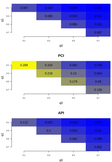
Estimands Related to Biomarker Evaluation

Recently, numerous amount of research effort are devoted to evaluating markers that can predict a patient’s chance of responding to a treatment. Usually we name these kinds of markers as biomarker. It is known that the treatment selection markers, may be called “predictive” (Simon, 2008) or “prescriptive” (Gunter et al., 2007) markers, have the possibility to improve patient outcomes and reduce medical costs by restricting the treatment used to subjects that seems most likely to have benefit. Since these biomarkers are useful, it is important to provide methods to evaluate the biomarkers.

(41)

Table 2.5: Monte Carlo estimates of the mean width of confidence intervals for the main effect of treatment at the 95% nominal level. The rows represent different methods of constructing CIs: (i) the n-out-of-n centered percentile bootstrap (CPB); (ii) the projection confidence interval (PCI); (iii) the m-out-of-n bootstrap; (iv) the proposed adaptive projection interval (API). Estimates are constructed using 200 datasets of size 150 drawn from each model, and 1000 bootstraps drawn from each dataset. Examples are designated NR=nonregular, NNR=near-nonregular, R=regular.

Q-learning Ex.1 Ex.2 Ex.3 Ex.4 Ex.5 Ex.6 Ex.A Ex.B Ex.C

A1 coefficient NR NNR NR NNR NR R R NR NNR

CPB 0.38 0.39 0.42* 0.42* 0.45 0.44 0.45 0.43* 0.42*

PCI 0.79 0.79 0.87 0.87 0.92 0.82 0.90 0.87 0.87

MOFN 0.77 0.79 0.71* 0.72* 0.95 0.44 1.35 1.30 1.32

API 0.41 0.42 0.49 0.48 0.46 0.44 0.53 0.54 0.48

One comprehensive approach to evaluating markers for treatment selection is proposed by Janes et al. (2014). Suppose we have two treatment options, which are denoted as treatment (T = 1) and no treatment (T = 0). Define D ∈ {0,1}, a binary indicator of an “adverse event”, which is the clinical outcome of interest within a specific time-frame following treatment assignment. For example,Dmay be chosen to represent an indicator of treatment-associated toxicity or death. We useY to denote a marker that is measured prior to treatment provision. The question here is whether Y useful for identifying a group of subjects who can avoid treatment. Define the absolute treatment effect given marker value Y as:

∆(Y) = P r(D= 1|T = 0, Y)−P r(D= 1|T = 1, Y).

The treatment rule is defined as following: do not treat if ∆(Y) <0. Refer to subjects with ∆(T)<0 as marker−negatives, and ∆(Y)>0 asmarker−positives. Following the notations from Janes et al. (2014), the useful measures are listed below:

• Average benefit of no treatment among marker-negatives,

(42)

• Average benefit of treatment among marker-positives,

Bpos = P r(D = 1|T = 1,∆(Y)>0)−P r(D= 1|T = 0,∆(Y)>0) = E(−∆(Y)|∆(Y)>0)

• Proportion marker-negative, Pneg =P r(∆(Y)<0)

• Decrease in population event rate under marker-based treatment,

Θ = P r(D= 1|T = 1)−[P r(D= 1|T = 1,∆(Y)>0)P r(∆(Y)>0) +P r(D= 1|T = 0,∆(Y)<0)P r(∆(Y)<0)]

= E(−∆(Y)|∆(Y)<0)·P r(∆(Y)<0) = Bneg·Pneg

In fact, the measure Θ, or its variation, has been advocated as a global measure of marker performance in many papers (Song and Pepe, 2004; Gunter et al., 2007; Janes et al., 2011; McKeague and Qian, 2011; Zhang et al., 2012b). Our target here is to construct a (1−α−η)×100% CI for Θ. Given data consisting of observations (Yi, Ti, Di), i= 1, ..., n, a general linear regression risk model (e.g. logistic regression) with an interaction between T and Y is used:

g(P r(D = 1|T, Y)) =β0+β1T +ψ1Y +ψ2T Y.

The corresponding estimator of ∆(Y) then can be defined as: ˆ

∆(Y) =g−1( ˆβ0+ ˆψ1Y)−g−1( ˆβ0+ ˆψ1Y + ˆβ1T + ˆψ2T Y).

Hence, the estimator for Θ is ˆ

Θ = Bnegˆ ·Pnegˆ

= En{−∆(Yˆ )|∆(Yˆ )<0}En(1_∆(ˆ _Y₎_<₀),

whereEn denotes the empirical expectation. The non-smooth region here satisfiesβ1T+

(43)

In this simulation study, we assume logistic regression model for g(P r(D= 1|T, Y)). Here is the simulation setting: TreatmentT is from bernoulli distribution with probability equals to 0.5. Marker Y is from mixed normal distribution with p.d.f defined as:

f(y) = p·φ(y; 0, c1) + (1−p)·φ(y; 0, c2),

whereφ represents normal density andpis the proportion has values between (0,1). We fix the variance ofY at 1, and define the variance ratio k = c2

c1. So during simulation, we

vary the distribution of Y through tuning the two parameters,k andp. The data gener-ation for the adverse event Dfollows the logistic regression model, where the parameters ψ1 =ψ2 = 1, and β0, β1 is defined by two tuning parameters q0, q1 satisfying that:

q0 =

1 1 +e−β0,

q1 =

1 1 +e−(β0+β1),

where the values of q0 and q1 fall in (0,1). Because q0 is related to the probability of

the adverse event for people with treatment andq1 is the probability of adverse event for

people without treatment, we define q1 ≤ q0 such that our setting is making sense. In

the simulation, let q0 = 0.1,0.3,0.5,0.7, q1 = 0.1,0.3,0.5,0.7 with q1 ≤ q0. Parameters

for markerY are defined by: k = 4 andp= 0.8. The sample size will be fixed atn= 100 with bootstrap replication B = 500 ,and monte carlo replication N rep= 200.

(44)

CPB

q0

q1

0.1 0.3 0.5 0.7

0.7 0.5 0.3

0.1 _0.935 _0.93 _0.88 _0.765

0.935 0.925 0.92

0.955 0.915

0.965

PCI

q0

q1

0.1 0.3 0.5 0.7

0.7 0.5 0.3

0.1 ₁ ₁ ₁ ₁

1 1 1

1 1

1

API

q0

q1

0.1 0.3 0.5 0.7

0.7 0.5 0.3

0.1 0.965 0.975 0.98 0.955

0.92 0.965 0.97

0.98 0.97

0.98

(45)

CPB

q0

q1

0.1 0.3 0.5 0.7

0.7 0.5 0.3

0.1 _0.087 _0.034 _0.009 _0.003

0.095 0.043 0.014

0.085 0.031

0.067

PCI

q0

q1

0.1 0.3 0.5 0.7

0.7 0.5 0.3

0.1 _0.288 _0.154 _0.081 _0.038

0.218 0.13 0.064

0.179 0.09

0.135

API

q0

q1

0.1 0.3 0.5 0.7

0.7 0.5 0.3

0.1 0.112 0.052 0.019 0.007

0.1 0.054 0.02

0.082 0.039

0.063

(46)

2.5

Discussion

In this section, we have illustrated the problem of non-regularity in a class of estimands defined as θ∗(β∗) = Es(X1, β1∗)g(X2, β2∗), where s(·) is smooth, and g(·) is non-smooth

in a region Q(X,β∗₎. We reviewed the existing approaches to construct CIs for this class

of estimands, and discussed the limitation of these current methods. We proposed an adaptive projection interval (API) method to construct a asymptotic valid (1−α−η)×

100% confidence interval for these estimands. The API is an adaptive method that is motivated from projection confidence interval proposed by Robins (2004). The double bootstrap procedure is used to tun the important parameterλn in API. The API has the advantage of being easy to understand, and simple to program. For illustration, we gave four different simulations: toy example, one-stage value function, first stage coefficients in multi-stage Q-learning, and biomarker evaluation. These empirical studies suggest that API always provide valid coverage rate for the estimands.

(47)

Chapter 3

Case Study for STEP-BD

(Systematically Treatment

Enhancement Program for Bipolar

Disorder)

3.1

Introduction of STEP-BD Study

Bipolar disorders are a group of chronic lifelong recurrent psychiatric disorders charac-terized by episodic shifts in mood, energy, social and vocational functioning, and activity levels (Phillips and Kupfer, 2013). Worldwide, bipolar disorders are a leading cause of disability (Vos et al., 2013) and associated with a substantial economic burden on society (Kleine-Budde et al., 2013). Standard antidepressant medications have been proved to be effective for acute and long-term treatment of unipolar depression (Bauer et al., 2013); however, supporting evidence for the inclusion of standard antidepressants in the acute and long-term treatment of bipolar depression is more limited and controversial (Grunze et al., 2010; Pacchiarotti et al., 2013).

(48)

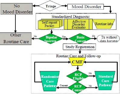
Figure 3.1: Registration procedure for STEP-BD study.

(49)

dis-Figure 3.2: Different pathways in STEP-BD study.

order: Acute Depression Randomized Pathway (RAD); Acute Depression Psychosocial Intervention Pathway (PAD); and Refractory Depression Pathway (REFD). If patients are unwilling to consent to one of the RCPs they remain in the SCP. In general, the de-cision of pathway (SCP versus RCP) is based on both the doctor’s and patient’s opinion. In STEP-BD, patients could switch pathways based on doctor’s or their own preference as well as inclusion and exclusion criteria. Figure 3.2 shows the diagram of STEP-BD study.

In this chapter, we analysis datasets from both randomized trails and observational trails. Section 3.2 is a case study for acute depression randomized pathway (RAD). Section 3.3 is the data analysis for observational acute depression pathway (SAD). Section 3.4 ends with discussion.

3.2

A Reanalysis of RAD using

Q

-learning

(50)

3.2.1

Acute Depression Randomized Pathway (RAD)

(51)

Figure 3.3: At the beginning (stage 1), there are 365 patients in total. 85 patients take Bupropion, 93 patients take Paroxetine and 187 patients take placebo. After 6 weeks, 104 patients’ information are lost. Only 78 patients are tracked with non-response at the end of stage 1. At stage 2, patients with non-response are assigned to secondary treatment intervention. Patients taking Bupropion or Paroxetine at stage 1 will increase current doses. But Patients taking placebo at stage 1 will be assigned Bupropion or Paroxetine.

Response for a given subject was defined as at least 50% improvement over their initial SUM-D score and not meeting the DSM-IV criteria for hypomania or mania. Scores on the continuous symptom subscale for depression (SUMD) range from 0 to 22, with higher scores indicating more severe symptoms. Both SUM-D and SUMM (symptom subscale for mood elevation, SUMM scores range from 0 to 16) are part of the modified Clinical Monitoring Form for mood disorders (Sachs et al., 2002).

(52)

evaluate DTRs (dynamic treatment regimes). In the next section we will formalize the notion of an optimal DTR and introduce a regression-based approach called Q-learning for estimating an optimal DTR from a SMART.

3.2.2

Dynamic Treatment Regimes and

Q

-learning

The effective management of a chronic illness requires ongoing personalized treatment (Wagner et al., 2001). Dynamic treatment regimes (DTRs) formalize clinical decision making as sequence ofdecision rules, one per treatment decision, that map patient infor-mation to a recommended treatment. An optimal DTR yields the minimal mean outcome when applied to assign treatment to a population of interest. One method for estimating an optimal DTR from observational or randomized study data is Q-learning (Murphy, 2005a; Schulte et al., 2012). Q-learning is an approximate dynamic programming algo-rithm that can be viewed as an extension of regression to multi-stage decision problems (Nahum-Shani et al., 2012). As our focus is the application of Q-learning to