Continuous Flow Microfluidic Separations.

(1)

ABSTRACT

SOOHOO, JEFFREY ROBERT. Continuous Flow Microﬂuidic Separations. (Under the direction of Glenn M. Walker.)

The goal of this research is to investigate novel methods for separating microscopic particles. Sorting complex mixtures of microscopic particles into subsets is a common process in many fields of research such as pharmaceuticals, environmental science, food science, military, cosmetics, agriculture and bio-medicine. This sorting step is often the most time consuming and laborious part of sample preparation. Microfluidics are espe-cially appropriate for separations at this scale because they offer significant advantages over conventional cell separation techniques such as reduced labor, less reagent usage, improved repeatability, smaller lab footprint, lower capital equipment cost and small sample sizes.

(2)

9.13 over unconcentrated blood.

Particle flux is an important factor for many microfluidics applications (e.g., separa-tions) and up to this point little attention has been paid to particle introduction. Delivery of a constant flux of particles into a microfluidic device is a challenge. Injecting parti-cles from syringe pumps, through small bore tubing, into microfluidic devices produces a varying and complex particle flux over time. A few methods have been reported in the literature for introducing particles into microfluidic devices. We characterized some of these methods and found that particle flux varied widely over time, by as much as seven fold. We then presented some useful methods for producing a constant rate of particles to a microfluidic chip. We found the most effective method for providing a constant flux was to use a density-matching solution and to eliminate all tubing.

The most common method for separating leukocytes from whole blood is through chemical lysis. However, lysis is a harsh method of separation and can alter the results of downstream analyses. In order to minimize the effect of lysis on the leukocytes we fabricated a microfluidic cytometer to characterize erythrocyte lysis kinetics. Diffusive transport coupled with laminar flow was used to control the concentration and exposure time of the lysis reagent to erythrocytes. Standard clinical practice is to expose ery-throcytes to lysis reagent for 10 min. Under optimum conditions we achieved complete erythrocyte lysis of a blood sample in 0.7 seconds. A maximum lysis reaction rate of 1.55 sec-1 _{was extrapolated from the data. Lysis began after 0.2 seconds and could be}

initiated with a lysis reagent concentration of 1.0% (68.5 mM).

(3)

bubbles of the same size but of insufficient quantity. Microfluidic particle separations using secondary flows were investigated for sorting microbubbles. These methods have been shown to be effective at separating solid particles but were found to damage the bubbles. An alternative means of generating secondary flows to avoid damage to bubbles was proposed.

Finally, we fabricated a microﬂuidic device that sorted microbubbles based on their buoyancy to capture a subset of bubbles of 6 – 7.5 µm in diameter. Microbubbles with

(4)

(5)

Continuous Flow Microﬂuidic Separations

by

Jeﬀrey Robert SooHoo

A dissertation submitted to the Graduate Faculty of North Carolina State University

in partial fulﬁllment of the requirements for the Degree of

Doctor of Philosophy

Biomedical Engineering

Raleigh, North Carolina

2014

APPROVED BY:

Michael Ramsey Paul Dayton

Brooke Steele Orlin Velev

(6)

DEDICATION

This dissertation is dedicated to the immediate and extended SooHoo clan who encouraged and supported education, my wife Jennifer who encouraged and supported

(7)

BIOGRAPHY

Jeffrey R SooHoo received his Bachelors of Engineering degree in 1993 from Hofstra Uni-versity in Hempstead, NY with a major in Bioengineering. After graduation Jeffrey went on to work at the Naval Research Laboratory in Washington, DC. At the NRL he worked on computer modelling of chemical kinetics, and the design of firmware, electronics, and environmental control systems for a wide range of biosensors. Additionally he developed models of electronic neural networks for image processing.

In the Fall of 1996, Jeﬀrey entered the Department of Biomedical Engineering at Rutgers University in Piscataway, NJ. His specialization was Medical Instrumentation and his major area of research was in human computer controls. He graduated with a Masters of Science in January 1998.

(8)

ACKNOWLEDGEMENTS

There are numerous people who have worked with me some whom I would like to ac-knowledge here:

My advisor: Glenn Walker

My committee: Dr. J. Michael Ramsey, Dr. Orlin Velev, Dr. Paul Dayton and Dr. Brooke Steele

Fellow current and former graduate students: Dr. Adrian O’Neil, Dr. Joshua Herr, Dr. Ben Moody, Dr. Vindya Kunduru, Dr. Jason Streeter, and Amy McPherson

Other people who have provided technical knowledge and support: J.P. Alaire, Dr. Susan Bernaki, Richard Greene, Steve Callender, Stefan Ufer, and Dr Ben Hui-Liu

The staﬀ who have helped me though the process: Linda Simmerson, Nancy McKin-ney, Jennifer Allen, Rekha Balasubramanyam, Stephanie Gootnick and Vilma Berg.

(9)

LIST OF TABLES

Table 2.1 Comparison of the separation eﬃciencies of zero, one, and two interface microscale and macroscale ATPS. A correlation exists between surface area-to-volume (SAV) ratio and the degree of leukocyte concentration. The fold-increase was calculated with respect to the unconcentrated control blood sample. All measured values are sample means plus or minus one standard deviation with n= 3. . . 21

Table 3.1 Table of Injection Schemes . . . 40

(12)

LIST OF FIGURES

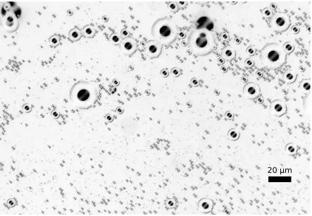
Figure 1.1 This image demonstrates the diﬃculty in separating white blood cells (WBCs) from red blood cells (RBCs), which outnumber WBCs by about 1000:1. The stained WBCs appear darker than the RBCs. Cells are approximately 10 µm in diameter. . . 3

Figure 1.2 Image of unsorted bubbles ranging from approximately 0.7 to 20 µm. 9

Figure 2.1 A cell at a two-phase interface experiences forces from the electrostatic potential (EP) and surface energy (SE) of the phases. Phosphate ions separate unevenly between the two-phases generating a positive po-tential in PEG relative to Dex. Diﬀerential surface energies γCell-Dex,

γCell-PEG, andγPEG-Dex between the phases and the cell will determine

its ﬁnal position. Surface energy diﬀerences cause blood cells to move into the Dex phase within the PEG-Dex system. Gravitational forces on cells are small relative to interfacial forces and are neglected here. 14 Figure 2.2 A) Whole blood is exposed to one interface, represented by the dashed

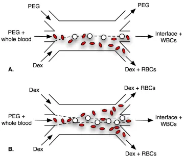
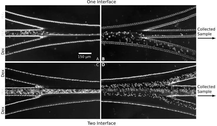
line, in the PEG-PEG-Dex conﬁguration. The leukocytes (WBC) pre-fer the interface while erythrocytes (RBC) migrate to the Dex. B) The two stream interface increases the surface area that blood is exposed to, resulting in more eﬀective leukocyte concentration. . . 19 Figure 2.3 The one interface setup consisted of a PEG-PEG-Dex pattern. A)

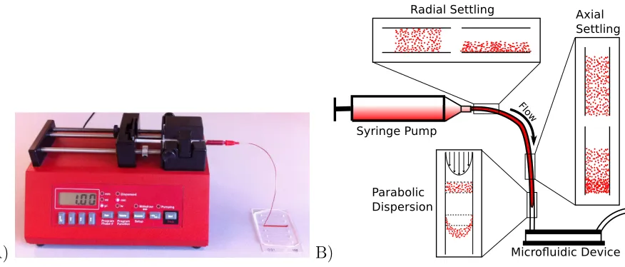
Blood was introduced in the middle stream and B) erythrocytes mi-grated to the Dex by the end of the channel. C) Blood was introduced into the two interface device (Dex-PEG-Dex) which provided twice the surface area for erythrocyte migration, as shown in D). . . 23 Figure 3.1 A) Typical setup for particle injection. Particles are often suspended in

a small volume syringe (e.g., 1 ml) mounted horizontally into a syringe pump connected to the device through tubing that meets the syringe horizontally and the microfluidic device vertically. B) Injection flux is a product of particle behaviour in small bore tubing, a combination of radial settling, axial settling and parabolic dispersion. . . 29 Figure 3.2 Diagram of axial settling in a vertical flow chamber. A) For particles

that are neutrally buoyant the flux is equal to the concentration, C, multiplied by the volumetric flow rate, Q. B) The addition of settling adds flux in proportion to the cross-sectional area, A, and settling velocity, VS. C) Model of axial settling with a cross-sectional area

(13)

Figure 3.3 A) Diagram of radial settling in horizontal tubing. The reduction in particle ﬂux is represented by a circle descending at a rate equal to the settling velocity. The original area is equal to the cross-sectional area of the tubing, AT. In time, t, the circle descends a distance tVs. R is the radius of the tube and θis the angle of the cord used in calculating

the overlapping area,AS. The fraction of remaining available particles was modelled as the overlapping area divided by the original area. B) The model assumed a constant settling rate of VS = 90.7 µm min-1, a tubing diameter of 508 µm and complete adhesion of the particle to

the tubing wall. Due to the small diameter of the tubing the particles settle quickly. . . 32 Figure 3.4 A) Diagram of parabolic dispersion in tubing. The parabolic ﬂow

pat-tern of pressure driven flow has a maximum velocity at the center of the tubing of twice the mean velocity and zero at the walls. Assuming the particles are evenly distributed in the fluid, the count past a down-stream observation point is proportional to the area of the parabolic section, AP, divided by the area of the tubing, AT. B) Model of parabolic dispersion. After a short delay for the sample to arrive at the observation point, flux asymptotically approaches the normalized value. If the plug is finite in length, the trailing edge alters the flux in a similar but negative way when it arrives at the detection area as shown by dashed line. . . 34 Figure 3.5 Model combining radial and axial settling and parabolic dispersion.

The initial increase is due to parabolic dispersion and axial settling, the tail is due to a combination of a decrease due to radial settling and spreading by parabolic dispersion. . . 36 Figure 3.6 Results from diﬀerent pump and device arrangements. A) The control

(14)

Figure 3.7 Active methods investigated to prevent settling in the syringe. A) Syringe pump on a rocker with metal sphere in the syringe to mix the contents of the tubing. B) Rotating the syringe to reduce radial settling in the syringe and tubing. C) Cell counts over time for active mixing methods. Both methods caused wide variations from handling the syringe and tubing. The unexpectedly high counts are likely caused by particles being counted multiple times as the vigorous movement of the tubing moves the particles in both directions past the detector. . 38 Figure 3.8 A) Experimental set up using an on-chip reservoir instead of tubing

to eliminate parabolic dispersion. B) Addition of air pumped into the reservoir to mix sample reducing axial settling. C) Results from three experiments using the reservoir. The reservoir alone demonstrated axial settling. Bubbling into the reservoir incompletely reduced the effect of settling. The addition of Optiprep made the cells neutrally buoyant eliminating settling and provided a constant flux of cells. . . 39 Figure 3.9 Plug introduction into a microfluidic device. A) The microfluidic

de-vice consisted of an input for the particle sample and a second input for buﬀer that focused the sample stream to the center of the device. B) Setup for control dispersion experiments. A plug of sample in the tubing is pushed through the device and travels a short distance before being quantiﬁed by a cytometer. . . 43

Figure 4.1 Flow diagram of device. Vacuum was applied to the outlet channel, which drew ﬂuid through the three inlets in a pre-deﬁned ratio based on inlet resistances. Data were collected at measurement points 1 mm apart, providing a repeatable and high time resolution picture of ery-throcyte lysis. . . 51 Figure 4.2 The molecular structure of ethyl-hexadecyl-dimethyl azanium bromide,

the ingredient in Zap-OGLOBIN II that lyses erythrocytes. . . 52 Figure 4.3 Diagram of experimental setup. The device was placed on an X-Y stage

and a laser was directed to the collection points. At each measurement point forward scatter data was collected, ﬁltered, digitized and stored for later analysis. . . 55 Figure 4.4 Comparison of computational model against chemical model for lysis

reagent flow and diffusion in a microchannel. A) Section of entire de-vice that the following images represent. B) Photo using fluorescein as model for Zap-OGLOBIN II. C) Computational model of lysis solution concentration. . . 57 Figure 4.5 The calculated and experimental concentration profiles of fluorescein

(15)

Figure 4.6 Longitudinal model results at lysis solution ﬂow rates of 1.0, 0.5, 0.25, and 0.125 µl/min. A) Highlighted cell paths. Plots of lysis reagent

concentration as seen by cell B) after lying solution sample intersection and C) after intersection of diluting buﬀer. . . 59 Figure 4.7 Graph of exposure vs cell count for four diﬀerent lysis solution

concen-trations. A) 0% concentration plotted vs distance downstream. Each line represents a different flow rate. B) 2.5%, C) 5%, and D) 25% concentration plotted against time. For each concentration the lysis rates were fit to lines taken over as a subset of the entire line start-ing when the remainstart-ing cells dropped below, and stayed below, 75%. Measurements were not taken over the 3 mm bend. . . 62 Figure 4.8 A) Graph of the cell counts at the lowest concentration at the highest

ﬂow rate. The cell count drops below the 75% threshold, representing the start of lysis, at 0.2 seconds. At this time the concentration of lysing solution the cells are in is 1%. . . 64 Figure 4.9 Plot of average times to complete lysis for each concentration. Using

the X-intercept of the linear ﬁts of Figure 4.7 we calculated how long lysis took to complete at each concentration and ﬁtted the data to the equation y=Ax−1₊_B. . . 64

Figure 4.10 Lysis rate vs concentration ﬁtted to power law equation. k = 0.71 and m = 0.25. . . 66

Figure 5.1 Inertial lift is a balance of the wall effect force,FW, and shear gradient force, FS, on a particle in a small channel. These forces will cause particles to line up at fixed distances from the channel walls. . . 71 Figure 5.2 Fluid velocities acting on particles in Dean flow. VC is the velocity due

to centrifugal force which is larger for fast moving fluid in the center of the channel. VL is the lift velocity of the fluid that was displaced by the center fluid. VB is the added velocity due to the buoyancy force for particles less dense than the fluid. . . 71 Figure 5.3 Spiral Dean flow design. Sample is introduced into the inner side of

the curved channel. Large particles are held to the the inner side by the inertial forces while smaller particles migrate outwards in the Dean ﬂow. . . 73 Figure 5.4 Bead sorting output. Beads are moving from left to right in the images.

On left is an image of the exit channel showing 0.4 µm beads. The

small beads traversed the entire width of the channel and exited via the outer exit. On right is the path of 4.0 µm beads. The majority

(16)

Figure 5.5 Bubble sorting results. The unsorted input had a wide spectrum of sizes from 1 to 13 µm. The medium and large exits were combined in

this experiment. The large bubbles did not arrive at any of the exits. The increase in the amount of small bubbles suggests that the large bubbles broke down into multiple smaller bubbles. This size cut-oﬀ was approximately 4.2 µm. . . 78

Figure 5.6 Similar to the recirculation generated with Dean flow, on left, sec-ondary flows can be generated using electro-osmotic flow (EOF) in a straight channel, on right. In this method the primary flow is inde-pendent of the secondary flow which would avoid the high pressures necessary in Dean flow. . . 80 Figure 6.1 Schematic of the device and its key parts. Bubbles enter from the left

at the middle of the larger channel and all move laterally at the same horizontal velocity as the fluid flow, Vf. In the main channel bubbles rise due to their buoyancy, Vb, with larger bubbles rising faster than smaller bubbles. The bubbles are caught in traps at locations designed to match bubbles of different sizes. The smallest bubbles pass all of the traps and exit the device. . . 86 Figure 6.2 Graph of the bubble travel distance as a function of flow velocity and

bubble diameter for a 0.5 mm rise distance. Travel distance is propor-tional to ﬂow velocity and decreases with the square of bubble diam-eter. Dashed lines signify travel distances between 20 and 140 mm in 20 mm increments. Bubbles sized between 6 and 7.5µm were targeted

and a limit of 50 mm maximum travel distance was imposed by the fabrication method. For 6 µm bubbles to be captured at 50 mm a

ﬂow velocity of 2.2 mm s−1 was required and led to a travel distance

of 32 mm for 7.5 µm bubbles. These points are shown by the white

(17)

Figure 6.3 Design of bubble sorting microfluidic device with critical dimensions and computational model of flow through the device. Buffer and bub-ble solutions entered from left. The buffer solution focused the bubbub-ble solution to the center of the stream so that all bubbles started at approximately the same height and rose through the same distance. Bubbles larger than size of interest were caught in the first 20 traps. The large trap captured the bubbles of the size of interest and bubbles smaller than that exited at the end of the last trap. The 50 mm and 32 mm distances are where bubble trajectories for 6 and 7.5 µm meet

the top of the main channel. In the main channel there is an even flow up to the trap of interest. There is a negligible amount of flow in to the first 20 traps so bubbles entering the traps do so only under the influence of buoyancy. . . 89 Figure 6.4 Photograph of experimental setup. The microfluidic device is levelled

and mounted on a vertical board which rests atop a dual channel sy-ringe pump. Buﬀer and unsorted bubble sample were introduced ver-tically from the syringe pump. . . 92 Figure 6.5 Representative images of traps for data analysis taken of trap 15. A)

is the raw image and B) shows the results of the image processing in which each detected bubble was highlighted in a hexagon and sized. Bubbles were sometimes missed if they were out of focus, too small or on the edge of the photograph. . . 94 Figure 6.6 Size spectra from the ﬁve experiments combined. The mean and

stan-dard deviation of the bubble diameters were calculated and plotted for each trap. The trap of interest was the second to last trap. The expected diameter range for each trap is highlighted in red. . . 95 Figure 6.7 Histogram of bubble size for each of the three regions: traps 1-20, trap

21 and trap 22. The data from the ﬁve experiments were combined. Bubbles larger than 7.5 µm were expected in the ﬁrst 20 traps. Those

traps were combined into one result. The trap of interest was number 21 and trap 22 was the waste and excess buﬀer. The peak size for trap 21 was approximately 6 µm with a narrow range as expected. . . 97

Figure 6.8 Bubble diameter and buﬀer viscosity are both signiﬁcantly dependent on temperature. The temperature used in the experiments was 25 ◦C.

By increasing the temperature the viscosity decreases and the bubble diameter increases. . . 102 Figure 6.9 Graph of bubble terminal velocity as a function of temperature.

(18)

Chapter 1 Introduction

1.1 Continuous Flow Microfluidic Separations

(19)

(20)

1.2 Blood Cell Separations

Microscopic biological particle separations often involves cells. We used blood cells as a model in this research because of their availability, importance, prior research on, and diversity of content. Blood is one of the most valuable patient samples that can be analyzed. The enumeration of leukocyte populations within peripheral blood provides valuable clinical information to physicians about the status of a patient. For example, HIV and leukemia can both be diagnosed and monitored by evaluating leukocyte sub-populations. While leukocytes are the most clinically-relevant cell population in whole blood, they are greatly outnumbered by erythrocytes. Typical red blood cell (RBC) counts are 4–6×106_/_µ_{l while white blood cell (WBC) counts are 4.5–10}_×₁₀3_/_µ_{l, which}

is a ratio of approximately 1000:1 RBCs to WBCs (see Figure 1.1).

(21)

lysing the erythrocytes and separating the leukocytes from the rest of the sample by centrifugation. Centrifugation requires milliliters of sample, is time- and labor-intensive, and requires the use of trained personnel and specialized equipment. Lysing is done by mixing diluted whole blood with lysis reagent and incubating the mixture for 10 minutes followed by a fixing step. The disadvantage of current practice is that over-exposure to lysis reagent can reduce leukocyte counts, [8, 36, 62, 61] in some cases as much as 60% [35]. Furthermore, lysing reagents have been shown to affect the expression of CD adhesion glycoproteins on the leukocyte surface [96]. These surface markers are typically used for characterizing the remaining cells via flow cytometry [60]. Thus, next-generation point-of-care devices that perform leukocyte analysis will require alternative methods of partitioning blood that use smaller sample volumes and minimize damage to leukocytes. Separation of blood cells in microfluidic devices has recently become an active area of research. Microfluidics offers a control the the environment unachievable at the macroscale while requiring only a few microliters of sample. Many different microflu-idic blood separation methods have been demonstrated such as lateral displacement [43], filters [12], lysis [86], and hydrodynamic separation [107]. For an overview of microfluidic blood separation methods see the reviews by Toner et al. [97] and Hou et al.[42]. While each method is capable of isolating cells, they also have disadvantages which must be weighed for the envisioned application.

(22)

Since then ATPS has been shown to be eﬀective at separating erythrocytes based on age [99] and species [100]. ATPS has also been used to analyze the surface charge proper-ties of blood cells [76, 98] and to fractionate leukocyte subtypes [103, 102, 67, 28, 58]. Leukocyte fractionation has traditionally been done using a multi-stage ATPS approach called counter current distribution (CCD) that can improve results. Separating based on cell and liquid surface properties would be a good alternative to using harsh chemicals to essentially dissolve unwanted cells.

(23)

prone to being disrupted by the high concentration of cells initially introduced to the device. Without a stable interface the effectiveness of the technique is greatly reduced. Approaches for injecting cells into microfluidic devices are often taken for granted. Some applications demand a constant flux of cells because uneven sample introduction can make rate-based measurements inaccurate (e.g., separations and kinetics studies), or as in ATPS, potentially alter separation properties. Other applications may be sensitive to clogging from large transients. To proceed we needed to find a means of injecting a constant rate of cells into the device.

Up to this point little attention has been paid to particle introduction. Delivery of a constant flux of particles into a microfluidic device is a challenge. Injecting particles from syringe pumps, through small bore tubing, into microfluidic devices produces a varying and complex particle flux over time. A few methods have been reported in the literature for introducing particles into microfluidic devices to minimize variation of particle flux including mixing[16], changing pump orientation,[77] syringe rotating,[48] viscosity modification[56] and density modification[80]. We characterized some of these methods and found that particle flux varied widely over time, by as much as seven fold. We then presented some useful methods for producing a constant rate of particles to a microfluidic chip. We found the most effective method for providing a constant flux was to use a density-matching solution and to eliminate all tubing.

(24)

studying lysis kinetics and performing lysis on samples. The exquisite control that micro-scale features give over diffusion and cell position allow one to minimize the amount of non-specific damage from the lysis reagent. Furthermore, the micro-scale environment can be tailored to maximize erythrocyte removal, resulting in purer leukocyte populations compared to current macro-scale methods. Elegant and clever microfluidic devices have been demonstrated for erythrocyte lysis [104, 86, 87, 82, 69]. However, only preliminary investigations into lysis kinetics in a microfluidic device have yet been performed.

1.3 Bubble Separations

In the second part of the dissertation we investigate separating non-biological particles based on size using bubbles as the model particle. Properties of non-biological particles are typically more homogeneous and as a result their size is often the basis of the sepa-ration. This eliminates surface properties and chemistry as a means of separation, which leads us to diﬀerent methods.

We use bubbles here as a model because of their clinical signiﬁcance. Encapsulated mi-crobubbles are currently used clinically as contrast agents for ultrasound imaging [59, 34]. Additionally, studies have demonstrated the potential of microbubbles or microbubble-based vehicles to aid in drug delivery, gene delivery, clot-disruption, or enhancing vascular permeability [6, 52]. The microbubbles used for ultrasound contrast agents are typically in the diameter range of 1–10 µm, and are often produced with techniques that lead to

(25)

the unique imaging and therapeutic capabilities of microbubbles.

The interaction between a microbubble and an ultrasound ﬁeld is highly dependent on the microbubble’s diameter [93] and hence recent research has focused on optimizing microbubble diameter and mono-dispersity in order to improve microbubble response to ultrasound. Acoustic studies on mono-disperse and size-sorted microbubbles have in-dicated the potential to improve ultrasound contrast imaging sensitivity substantially, based on adjusting microbubble size distribution alone [91]. For drug-carrier microbub-bles, there is additional desire to formulate particles with similar drug-loading and release characteristics, which are also related to vehicle size [41]. Finally, for safety purposes, bubbles larger than capillaries (> 8 µm diameter) need to be removed before injection

into a patient to prevent blood vessel obstruction.

The most common current methods of bubble generation for contrast agent generation are acoustic emulsiﬁcation (sonication), and mechanical agitation [59]. These methods yield a wide spectrum of sizes, from sub-micron to over 20µm in diameter [93], as shown

in Figure 1.2.

Several groups have explored the application of microfluidics to the precision genera-tion of encapsulated microbubbles [32, 41, 95, 94]. These methods have the capability to tailor the mean diameter by adjusting flow rates. Two of the most effective methods are T-junction systems [18] and co-axial electro-hydrodynamic atomization [73]. Although these techniques result in better size control than traditional bulk methods of microbub-ble formulation, they are limited by low production rates. The fastest rate is 105

/sec[21]

whereas macroscale sonication produces bubbles at a rate of1×1010

/min. At least1×108 bubbles are needed for imaging even a small laboratory animal [30], let alone a human.

(26)

20 μm

Figure 1.2: Image of unsorted bubbles ranging from approximately 0.7 to 20 µm.

sorting consists of a series of up to 14 centrifugation-resuspension steps. It is a time-consuming process, the results of which are dependent on technical aptitude. Preliminary work on ﬂotation based sorting was done in a long tube [51], but the reduction of the size spectrum was modest at best.

(27)

concentration of 10, 15 and 20 µm polystyrene beads at a throughput of greater than

1×106

/min [50]. The success in separating beads with this method did not translate to

separating bubbles. The method reduced the larger bubbles into smaller bubbles beyond usefulness due to large pressures developed by the high ﬂow rates in small channels. Finally, an alternate to generate the circulating transverse ﬂow using electro-osmotic was proposed but not investigated.

(28)

Chapter 2 Aqueous Two Phase Systems for Cell

Separation

2.1 Background

An emerging theme in microﬂuidics is the use of miniaturized devices for acquiring cellular-level diagnostic information from patient whole blood samples [55]. The abil-ity to concentrate leukocytes from whole blood is a prerequisite for most hematological analyses. A sample of whole blood contains ∼5×106

erythrocytes/µl which, if not

re-moved, can interfere with assays aimed at the less common leukocytes (∼104

/µl). Within

(29)

glycoproteins on the leukocyte surface. These surface markers typically used for charac-terizing the remaining cells via ﬂow cytometry [60]. Thus, next-generation point-of-care devices that perform leukocyte analysis will require alternative methods of partitioning blood that use smaller sample volumes and minimize damage to leukocytes.

Separation of blood cells in microfluidic devices has recently become an active area of research. Many different separation methods have been demonstrated such as lateral displacement [43], filters [12], lysis [86], and hydrodynamic separation [107]. For an overview of microfluidic blood separation methods see the review by Toner et al.[97]. While each method is capable of isolating cells, they also have disadvantages which must be weighed for the envisioned application. Of these methods only lysis has a specificity near 100% and even with its drawbacks it still remains the method of choice for leukocyte concentration.

One microfluidic separation method which has yet to be applied to blood is an aque-ous two-phase system (ATPS). ATPS have been demonstrated in microfluidic devices for separating plant cell aggregates [108], live/dead Chinese Hamster Ovary cells with fractionation efficiencies of up to 97% [70], and for protein purification [66]. However, no work has been done using ATPS to microfluidically separate leukocytes from erythro-cytes, even though these cells types are known to have different surface properties, which suggests ATPS should be a viable separation strategy.

(30)

been used to analyze the surface charge properties of blood cells [76, 98] and to fraction-ate leukocyte subtypes [103, 102, 67, 28, 58]. Leukocyte fractionation has traditionally been done using a multi-stage ATPS approach called counter current distribution (CCD) that can improve results.

Separation of blood components with ATPS at the macroscale requires large sample volumes and can take 20 minutes to complete. Often multiple separations are required to achieve well-sorted samples. Microfluidic devices can potentially enhance ATPS because the surface area-to-volume ratio of the streams is very large, decreasing the distance a cell must travel before coming into contact with a phase interface and potentially making separations faster. Microfluidics also allows for continuous cell separation, something that is difficult with traditional ATPS.

2.2 Theory

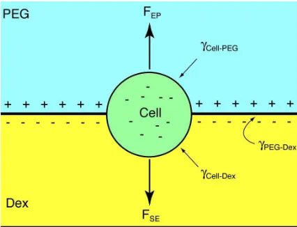
Each cell type has particular surface properties and net charge; within an ATPS each phase has a unique surface energy and charge. When a heterogeneous mixture of cells is placed in an ATPS, the distinctive characteristics of each cell determine its interaction with the phases, resulting in cell separation by type. The cells will position themselves in the most energetically favorable location within the system, which can be in either phase or at the interface between the phases. The forces acting on a cell within an ATPS result from electrostatic potential and surface energy [101, 33] and are shown in Figure 2.1.

(31)

Figure 2.1: A cell at a two-phase interface experiences forces from the electrostatic po-tential (EP) and surface energy (SE) of the phases. Phosphate ions separate unevenly between the two-phases generating a positive potential in PEG relative to Dex. Diﬀeren-tial surface energies γCell-Dex,γCell-PEG, and γPEG-Dex between the phases and the cell will

determine its ﬁnal position. Surface energy diﬀerences cause blood cells to move into the Dex phase within the PEG-Dex system. Gravitational forces on cells are small relative to interfacial forces and are neglected here.

no net charge, phosphate ions separate unevenly making PEG positive relative to Dex. If the generated electrostatic potential is large enough, it will interact with the surface charge of cells, driving them into the phase of opposite charge. Typical electrostatic potentials range from microvolts to millivolts and usually have less of an influence on cell separation than the surface energy. However, even relatively weak electrostatic potentials can generate strong electric fields over the short distances present in microfluidic systems, making this force potentially useful for cell sorting applications.

(32)

|γ(Cell-PEG)−γ(Cell-Dex)| > γ(PEG-Dex) (2.1)

then they will move into the phase in which they experience the lowest surface energy. Otherwise the cells will be held in place at the interface.

The magnitude of force experienced by a cell from ATPS surface energy is proportional to the cell surface area, surface properties and polymer concentration. By minimizing the PEG and Dex polymer concentrations, the diﬀerence between the surface areas of erythrocytes and leukocytes (∼ 140 µm2 _and

∼ 300 µm2_{, respectively) can be used to} concentrate the leukocytes. The erythrocytes have a lower surface energy and will quickly move into the Dex phase while the leukocytes, with a higher surface energy, will stay near the interface.

Microﬂuidics provides an advantage here because the large surface-to-volume ratio allows many cells to rapidly sample the interface and thus determine their placement either within the bulk phases or at the interface. The high viscosity of the phases and the microscale dimensions of the system ensure that Re≪1which will prevent turbulence

and allow smooth, continuous interfaces to be maintained. Furthermore, the laminar ﬂow present in microﬂuidic channels allows cells to be precisely positioned near the interface, further enhancing cell sampling of the two-phases.

2.3 Materials and Methods

2.3.1 Device Design and Fabrication

(33)

poly-created by spin coating negative tone photoresist to a height of 100 µm (SU-8 2100,

Mi-crochem Corp., Newton MA) on a silicon wafer. The photoresist was selectively exposed to ultraviolet light (BlakRay B-100a, UVP, Upland, CA) through a high resolution trans-parency containing the channel design. After the unexposed photoresist was removed via developer, a PDMS mold was cast oﬀ the master as follows (SYLGARD 184 Silicone Elastomer Kit, Dow Corning, Midland, MI). PDMS base and curing agent were mixed in a 10:1 ratio, degassed, and poured over the mold which was held in an aluminum foil boat. The PDMS was then cured at 125 ◦C for 15 min. Once the PDMS was removed

from the master, ports were cored out and the PDMS was bonded to a glass slide using an oxygen plasma treatment. Tygon tubing (Tygon S-50-HL, Cole-Palmer, Vernon Hills, IL) was inserted into ports, cored out with a blunt 16 gauge needle, and used to connect the microﬂuidic devices to syringe pumps.

The ATPS microdevices had three inputs which merged into a single main channel and then diverged into three outputs so that the number and position of the interfaces in the main microchannel could be controlled. Each of the input and output channels were 50 µm wide, merging into and diverging from, respectively, a 150 µm wide, 20 mm

long channel.

(34)

found that the instabilities limited the length of the main channel to 20 mm and the height to 100 µm. The width of the main channel was not considered because the thickness of

the center stream was controlled by the relative ﬂow rates between the channels.

2.3.2 Aqueous Two-Phase System

The two-phase system was prepared by combining PEG (Poly-Ethylene Glycol 8000, Fisher Scientiﬁc), Dex (Dextran MW 500,000, Fisher Scientiﬁc), 10× PBS (10×

Phos-phate Buﬀered Saline, Sigma) and deionized water in a conical tube to create a 50ml solution of 1x PBS, 4% w/w PEG and 5% w/w Dex. The PBS was added to ensure the phases would remain physiologically osmotic, providing a ﬁnal solution with 10 mM phosphate, 154 mM sodium chloride and a pH of 7.4. This concentration of polymers and salts was used for all experiments. The electrostatic potential generated by these salt concentrations was approximately 40µV [100] which is far too small to induce

move-ment in the blood cells during separation. The tube was shaken vigorously to break up large clumps of Dex and stored at room temperature overnight to ensure that the polymers were fully dissolved. PEG and Dex aliquots were extracted 500 µl at a time

using one milliliter syringes. Dex was extracted from the bottom of the tube and PEG was extracted from the top of the tube.

(35)

disappear about 4 mm downstream of the input channels. In both experiments, whole blood was ﬂowed in through the middle input channel and cells were collected at the middle output channel.

The one interface conﬁguration was created with a PEG-PEG-Dex stream pattern. In this approach a 10µl sample of whole blood was diluted into 500µl of PEG solution and

flowed through the middle input microchannel between streams of PEG and Dex. Input flow rates were adjusted via the syringe pumps so that the PEG-Dex interface exited into the center output channel, while minimizing the amount of Dex that was collected. The stream containing the blood sample had a flowrate of 1 µl/min and the outer streams

were adjusted as needed to position the interface, typically 0.7–2µl/min.

The two interface conﬁguration was created using a Dex-PEG-Dex stream pattern. Here, two outer streams of Dex were used to double the interfacial surface area that the blood cells suspended in the middle PEG stream were exposed to. Maintaining stable interfaces with two streams of high viscosity Dex required extra pumps at each of the Dex exit channels. The ﬂow rates were adjusted so that the PEG stream, with interfaces, was collected in the middle output channel.

Blood samples were prepared similarly in all of the experiments. One hundred micro-liters of whole blood were taken from a ﬁnger prick of the same volunteer and placed in an EDTA coated tube (K2-EDTA Vacutainer, Becton-Dickinson, Franklin Lakes, NJ). The ratio of erythrocytes to leukocytes was counted each time with a hemacytometer. The variation of the initial erythrocyte to leukocyte ratio among samples for all experi-ments was less than 7%. Ten microliters of blood were then taken from the EDTA tube and added to the appropriate syringe and mixed. Cells were always introduced into the device via the middle input. During each experiment approximately 50µl of eﬄuent was

(36)

(37)

a multiwell plate.

The erythrocyte and leukocyte populations were then counted on a hemacytometer. The hemacytometer and coverslip were cleaned with ethanol and Kim-wipes. After both pieces had dried, the coverslip was placed on hemacytometer and 10µl of cell solution was

aliquoted into the hemacytometer. The cells were counted and recorded as erythrocytes. Lysing solution (Zap-O Globin, Beckman Coulter, France) was added to the remaining sample and counting was repeated and the cell count was recorded as leukocytes.

For the macroscale ATPS, 10 µl of blood was placed in a 1.5 ml centrifuge tube

containing 500 µl of each phase, mixed well, and then allowed to sit for 30 min so the

phases could separate. All experiments were performed three times (n= 3).

2.4 Results and Discussion

Five diﬀerent experimental setups were tested for their ability to separate leukocytes from whole blood (Table 2.1). For the control, cell counts were taken directly from whole blood in EDTA-coated tubes and had an erythrocyte to leukocyte ratio of 949 ±64.9

(38)

Table 2.1: Comparison of the separation eﬃciencies of zero, one, and two interface microscale and macroscale ATPS. A correlation exists between surface area-to-volume (SAV) ratio and the degree of leukocyte concentration. The fold-increase was calculated with respect to the unconcentrated control blood sample. All measured values are sample means plus or minus one standard deviation with n = 3.

Macro- PBS No One Two

Control scale Only Intf. Intf. Intf.

RBC/WBC Ratio 949 ±64.9 707 ±570 528±247 594 ±144 188 ±107 104 ±12.8 WBC Enrichment 1.0 ±0.07 1.34 ±1.1 1.80±0.84 1.60 ±0.39 5.05 ±2.87 9.13 ±1.12

(39)

The macroscale experiment in a static ATPS resulted in both the erythrocytes and leukocytes migrating to the lower bulk Dex phase. Cells were carefully collected from the Dex side of the interface. The average ratio of erythrocytes to leukocytes was lower compared to the control (707±570), suggesting that the leukocytes preferred being near

the interface, most likely due to their larger surface area. These results also support the ﬁndings discussed below in which higher leukocyte concentrations were found in samples of the PEG-Dex interface from the microﬂuidic devices.

To create a one-interface microﬂuidic setup a PEG-PEG-Dex stream pattern was used. Blood was mixed with PEG and ﬂowed in through the middle stream. The blood cells were pinched against the Dex stream by the outer PEG stream, greatly reducing the time required for them to sample both phases compared to the macroscale ATPS (Figure 2.3a and 2.3b). Samples collected from this setup had an average erythrocyte to leukocyte ratio of 188±107, or a 5.05-fold increase in leukocyte concentration over

the control.

A two interface system was created with a Dex-PEG-Dex stream pattern and resulted in collected samples with an average erythrocyte to leukocyte ratio of 104±12.8, or a

9.13-fold increase over the control. The two interface system had an interfacial surface area double the one interface system and thus the interfacial surface area-to-volume ratio was four times greater than in the one interface system. This experimental setup created samples with slightly higher erythrocyte and leukocyte counts because the addition of a second interface increased the likelihood that blood cells in the middle stream would sample both phases (Figures 2.3c and 2.3d). Microﬂuidic methods which can further increase the surface area-to-volume ratios between the two phases should result in even higher concentrations of leukocytes.

(40)

150 µm A C Collected Sample Collected Sample De x De x PE G PE G PE G De x B D One Interface Two Interface

Figure 2.3: The one interface setup consisted of a PEG-PEG-Dex pattern. A) Blood was introduced in the middle stream and B) erythrocytes migrated to the Dex by the end of the channel. C) Blood was introduced into the two interface device (Dex-PEG-Dex) which provided twice the surface area for erythrocyte migration, as shown in D).

effects of hydrodynamic (i.e., non-interfacial) forces on leukocyte separation efficiency. In the first experimental configuration PBS was used in all three microchannels to quantify how flow alone affected erythrocyte and leukocyte concentrations in the middle collection channel. Compared to the control sample and macroscale ATPS, a lower erythrocyte to leukocyte ratio of528±247was observed. The reduced ratio of erythrocytes to leukocytes

(41)

diﬀused into the PEG and Dex streams. The PEG-PBS-Dex stream pattern resulted in a collected sample with an erythrocyte to leukocyte ratio of594±144, or a 1.6-fold increase

over the control. The separation in this arrangement is slightly less eﬀective than with the zero-interface all PBS pattern, which proves that the polymers themselves do not cause separation and that a distinct interface between phases is required to signiﬁcantly concentrate leukocyte populations within whole blood samples.

2.5 Conclusions

Microfluidic ATPS allowed us to create a precise, consistent fluidic environment with a stable interface in which we could carefully control the location of the cells and the position of the interface. More importantly, microfluidics allowed us to collect cells trapped at the interface, which is not practical with current macroscale ATPS methods. The ATPS surface area-to-volume ratio was large enough to quickly expose cells to the interface and increasing the ratio in the device boosted separation efficiency. However, maintaining a stable interface required a separate pump at each input. The interfaces within microfluidic ATPS were sensitive to slight pressure variations and could easily be disrupted if the flowrate was too large (greater than 10 µl/min) which limited the

throughput of separated cells.

(42)

interface.

The current device is targeted at separating white blood cells from whole blood, but any heterogeneous cell solution with a sufficiently high partition ratio can be fractional-ized and even sub-fractionalfractional-ized. For example, the serial devices need not perform the same separation. In such a configuration, each cascade would have a different two phase system that could pull out a different cell type from solution. These devices have the po-tential be used in any application in which sufficiently differing cells need to be separated (e.g., isolating circulating cancer cells or detecting bacteria).

(43)

Chapter 3 Maintaining a Constant Flow of

Erythrocytes

3.1 Background

Injecting micron-sized particles, such as cells or polystyrene beads, into microfluidic de-vices is a pervasive technique. Many microfluidic applications are insensitive to the rate at which particles are injected. However, some applications require a constant flux, such as measuring reaction kinetics. In addition, some procedures such as in ATPS, particle trapping and flow cytometery[3], become ineffective if the flux is too high (leading to clogging), necessitating control over particle flux.

(44)

den-sity modification[80]. Inertial flow is an emerging technique that can precisely space particles regardless of the input flux, [26] but this technique requires very fast flow rates that are not be suitable for many applications. Regardless of the approach, the particle flux over time is often taken for granted during experiments, and to date no comparison of the methods has been performed.

Most of the variability of particle flux is caused by two phenomena: parabolic dis-persion and particle settling. Parabolic disdis-persion is a product of pressure driven flow in small bore tubing, i.e. the middle of the flow stream is faster than at the edge. This has the effect of stretching the plug of sample over time. Particle settling has a different effect depending on if it is in the direction of flow or perpendicular to flow. Settling in the direction of flow causes an increase in particle concentrations as particles accumulate at the bottom of tubing or reservoir typically found at the entrance of a microfluidic device. This results in a linear increase in flux over time and to a level that depends on a combination of the settling velocity, flow rate and concentration. Settling perpendicular to flow will cause a decrease in flux as particles descend and adhere to the tubing walls. In small tubing, a decrease to a flux of zero can happen in just a few minutes. The combination of the two settling types with parabolic dispersion leads to complex flux transients.

(45)

3.2 Theory

In a typical setup for particle injection particles are suspended in a small volume syringe (e.g., 1 ml), mounted horizontally into a syringe pump connected to the device through tubing that meets the syringe horizontally and the microfluidic device vertically, as shown in Figure 3.1A. This setup exemplifies the three major sources of particle flux transients: radial settling in the horizontal section of tubing and in the syringe, axial settling in the vertical section of tubing and parabolic dispersion in narrow tubing, as shown in Figure 3.1B. Settling in the vertical section of the tubing increases particle flux while settling in the horizontal section reduces flux as particles stick to the tubing wall and parabolic dispersion stretches the plug of particles out also reducing flux.

3.2.1 Settling Models

Two models of settling, axial (with flow) and radial (perpendicular to flow), were devel-oped. These models assumed a sufficiently dilute mixture of particles in fluid such that the interaction between particles is negligible.

Axial Settling Model

For neutrally buoyant particles ﬂux past an observation point is simply the concentration multiplied by the volumetric ﬂow rate:

F =CQ (3.1)

whereF is the ﬂux,C is the concentration andQis the volumetric ﬂow rate. A schematic

(46)

A) B)

Figure 3.1: A) Typical setup for particle injection. Particles are often suspended in a small volume syringe (e.g., 1 ml) mounted horizontally into a syringe pump connected to the device through tubing that meets the syringe horizontally and the microﬂuidic device vertically. B) Injection ﬂux is a product of particle behaviour in small bore tubing, a combination of radial settling, axial settling and parabolic dispersion.

If particles are more dense than the fluid they accelerate downward and reach a terminal velocity. The acceleration phase of the descent is sufficiently short that it can be ignored. Settling in the same direction as the flow is termed axial settling. Given enough time, the flux, with the addition of axial settling, will be equal to the concentration multiplied by the sum of the bulk volumetric flow rate and settling velocity,VS, multiplied

by the cross-sectional area, A,

F =C(Q+AVS) (3.2)

as shown in Figure 3.2B.

(47)

K is a complex combination of flow rate, settling velocity and area of both the tubing and the entrance to the microfluidic device. For very small areas, like that found in tubing, and with sufficiently high flow rates (> 1 µl min-1_{) this effect is small. The use}

of a reservoir instead of tubing can increase the area by over a hundred fold making this the dominant effect on flux. For simplicity, the equation to model the increase in flux is reduced to

AS = 1 +Kt (3.4)

where AS is the unitless particle ﬂux multiplier due to axial settling.

Radial Settling Model

Radial settling occurs when particles settle perpendicular to the ﬂow direction. This typically occurs in the form of particles descending due to gravity in a horizontal tube and sticking to the bottom of the tube. To model radial settling we consider the cross-section of a tube initially evenly ﬁlled with particles. The particles all descend at the same velocity in the shape of a descending circle clipped by the original area representing the settling particles, as diagrammed in Figure 3.3A. The fraction of remaining available particles is equal to the overlapping area divided by the original area. In common 0.5 mm diameter tubing the particles can settle completely within a few minutes, as shown in Figure 3.3B.

To calculate the overlapping area we calculated the area between cord of a circle formed by the intersection of the two circles and the circumference of the circle and doubled the value. The equation for this area is:

(48)

A) F=CQ Q C Observation P oint A

B)F=C(Q+AVS)

C Q+AVS Observation P oint A C) 0 1 2 3 4 5 6

0 10 20 30 40 50 60

Normalized Particle Flux

Time [Min]

Neutrally Buoyant Particles Axial Settling in a Reservoir Model

Maximum Flux = C(Q+AV_s)

Figure 3.2: Diagram of axial settling in a vertical flow chamber. A) For particles that are neutrally buoyant the flux is equal to the concentration, C, multiplied by the volumetric flow rate, Q. B) The addition of settling adds flux in proportion to the cross-sectional area, A, and settling velocity, VS. C) Model of axial settling with a cross-sectional area

large in proportion to the ﬂow rate.

where AS is the overlapping area, R is the radius and θ is the angle of the cord.

The ratio of the overlapping area to the original area, which is equal to cross-sectional area of the tube, reduces to:

RS = AS

AT

= (

θ

2 −sin[ θ 2]cos[

θ 2])

π (3.6)

where RS is the unitless relative particle ﬂux multiplier at the output due to radial settling. Adding the ﬂuidic components to the model is done by calculating θ in terms

of the settling velocity, VS and time, t

θ

2 =cos

−1

tVs

2×R

(49)

A)

V_S

θ _R

t V_S

AT AS B) 0 0.2 0.4 0.6 0.8 1

0 2 4 6 8 10

Relative Particle Counts

Time [min]

Figure 3.3: A) Diagram of radial settling in horizontal tubing. The reduction in particle ﬂux is represented by a circle descending at a rate equal to the settling velocity. The original area is equal to the cross-sectional area of the tubing, AT. In time, t, the circle descends a distancetVs. R is the radius of the tube andθ is the angle of the cord used in

calculating the overlapping area, AS. The fraction of remaining available particles was

modelled as the overlapping area divided by the original area. B) The model assumed a constant settling rate of VS = 90.7 µm min-1, a tubing diameter of 508 µm and complete adhesion of the particle to the tubing wall. Due to the small diameter of the tubing the particles settle quickly.

3.2.2 Parabolic Dispersion Model

In a cylindrical channel, such as in the tubing connecting the syringe to the device, a plug of sample is stretched into a paraboloid. The maximum velocity of the paraboloid occurs at the center of the tubing and is twice the average velocity. The minimum velocity is zero at the walls. If the assumption is made that particles are evenly distributed within the solution, then the particle ﬂux past a downstream observation point is proportional to the area of the parabolic section divided by the area of the tubing, as shown in Figure 3.4A. Parabolic dispersion can be modelled by Eq. 3.8

P D= AP

AT

=

q

1− ∆x

tVM ax

(50)

where P D is the unitless particle ﬂux multiplier due to parabolic dispersion, AP is the cross-sectional area of parabolic section, AT is the cross-sectional area of the tubing, R the radius of the tubing,∆xis the distance between the start position of the leading edge

of the particle sample and the observation point, VM ax is the maximum velocity of the ﬂuid and t is time. After a delay, there will be a quick increase in counts asymptotically

to a peak. If the sample plug is finite (or has been truncated by radial settling) the trailing edge of the plug will pass the observation point with a slower decrease than the increase of the leading edge since the trailing edge has travelled further giving it a larger ’∆x’. An example of how parabolic dispersion effects flux is shown in Figure 3.4B.

3.2.3 Combined Model

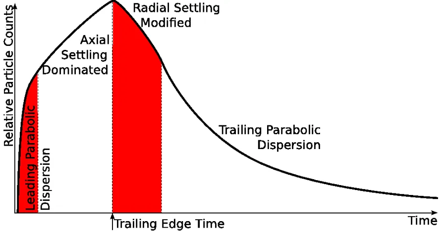
The three parts of the model for the typical setup, shown in Figure 3.1, combine in a straightforward way, as shown in Eq. 3.9. The initial part of the ﬂux, F, is a product of the initial concentration, C, the volumetric ﬂow rate, Q, parabolic dispersion multiplier,

PD and axial settling multiplier, AS. When the trailing edge of the plug (caused by radial settling, RS, in the horizontal part of the tubing) first arrives at the measurement point (TET, Trailing Edge Time) the concentration is reduced by the radial settling applied to parabolic dispersion. The result of combining all of these factors results in an initial fast increase due to parabolic dispersion that is then followed by a linear increase due to axial settling. The flux then decreases as the loss of concentration due to radial settling arrives at the detection point. The flux decays with a elongated parabolic dispersion shape modified initially by the radial settling. The combined model is shown in Figure 3.5.

 

 C×Q×P D×AS t <=T ET

(51)

A) ObservationPoint

Leading Edge Trailing Edge

AT

B)

0 0.2 0.4 0.6 0.8 1

0 5 10 15 20

Relative Particle Counts

Time [min]

Leading Edge Trailing Edge if Present

(52)

3.3 Experimental Design

We investigated eight different injection schemes and their effects on particle flux over time as described in Table 3.1. Each scheme was designed to analyze axial and/or radial particle settling prior to injection into the microfluidic device. The control scheme was a horizontally-mounted syringe in a syringe pump connected to a microfluidic device via 150 mm of small inner diameter (0.508 mm) tubing with a vertical drop of 100 mm, as shown in Figure 3.6A.

To isolate the two different types of settling, the positions of the syringe, tubing and device were modified. The effect of radial settling on particle flux was determined by winding the tubing into a horizontal coil, as shown in Figure 3.6B. The coil was kept at the same height as the entrance port of the microfluidic device so that the only vertical drop occurred in the port. The tubing volume was larger than 200 µl which provided

enough particles for an entire experiment. The effect of axial settling on particle flux was determined by mounting the syringe pump 150 mm above the chip, as shown in Figure 3.6A. In both experiments the syringe and tubing were filled just prior to running the experiment to minimize any pre-experimental settling.

In order to eliminate settling two active mixing strategies to keep particles suspended were attempted. In the ﬁrst set up the syringe pump (with syringe) was mounted on an automated rocking platform and rocked ±45◦at 0.5 Hz, as shown in Figure 3.7A. A 3 mm

diameter stainless steel shot was added to the syringe to aid in mixing of the sample. Tubing length was increased to 300 mm to accommodate the movement of the syringe. In the second set up, the syringe was manually rotatedin situ 180◦ each minute, as shown in

(53)

(54)

D) 0 0.2 0.4 0.6 0.8 1 1.2 1.4 1.6

0 10 20 30 40 50 60

Normalized Particle Flux

Time [Min]

Model of Particle Flux for Control Experiments

Coiled Control Vertical E) 0 0.5 1 1.5 2

0 10 20 30 40 50 60

Normalized Cell Flux

Time [Min]

Normalized Cell Flux for Control Experiments

Coiled Control Vertical

(55)

C)

0 1 2 3 4 5 6 7

0 10 20 30 40 50 60

Time [Min]

Normalized Cell Flux for Experiments with Tubing

Rocker with BB Rotated Syringe

Figure 3.7: Active methods investigated to prevent settling in the syringe. A) Syringe pump on a rocker with metal sphere in the syringe to mix the contents of the tubing. B) Rotating the syringe to reduce radial settling in the syringe and tubing. C) Cell counts over time for active mixing methods. Both methods caused wide variations from handling the syringe and tubing. The unexpectedly high counts are likely caused by particles being counted multiple times as the vigorous movement of the tubing moves the particles in both directions past the detector.

(56)

C)

0 1 2 3 4 5 6 7

0 10 20 30 40 50 60

Time [Min]

Normalized Cell Flux for Reservoir Experiment

Reservoir Only Reservoir Model Bubbling Optiprep Optiprep Model

(57)

Table 3.1: Table of Injection Schemes

Type of settling Radial settling Axial settling Radial settling Axial settling

Minimized in syringe in syringe in tube in tube/reservoir

Control N Y N N

Vertical syringe Y N Y N

Coiled tubing N Y N Y

Rotated syringe Y Y N N

Rocker with B-B Y Y Y N

On-chip well Y Y Y N

On-chip well + Bubbled Y Y Y Y

(58)

3.4 Materials and Methods

3.4.1 Microchip Fabrication

Glass microfluidic chips were fabricated using standard wet chemical etching techniques as described previously [65, 78]. Briefly, white crown glass substrates (B270) coated with chromium and positive photoresist (Telic Co., Valencia, CA) were patterned with the chip design by flood UV exposure using a custom photomask (Photoplot Store, Col-orado Springs, CO). After photoresist development (MF-319; MicroChem Corp., Newton, MA) and removal of exposed chromium (Chromium Etchant; Transene, Danvers, MA), channels were etched into the glass substrate using a dilute HF/NH4F solution (10:1

Buﬀered Oxide Etch; TransenE). The etched substrates were then diced and access holes made by powder blasting (Comco Inc., Burbank, CA). All glass was then thoroughly cleaned by sonication in a 5% solution of Contrad 70 (Fisher, Waltham, MA) for 10 min-utes, followed by immersion in Nanostrip 2X solution (Cyantek Corp., Fremont, CA) for 30 minutes. Etched glass substrates and glass covers were then hydrolyzed in a 2:2:1 solution of H₂O/NH₄OH/H₂O₂ for 30 minutes at 70◦C, followed by thermal bonding at

550◦C for ten hours. Threaded ports for connection to a syringe pump via PEEK tubing,

and reservoirs, 6.35 mm in diameter and approximately 100 µl in volume were bonded

to the top of the device with epoxy.

3.4.2 Data Collection

(59)

create a ﬂow cytometer, as shown in Figure 3.9B and as described elsewhere[40]. A 488 nm solid-state laser (40 mW) (Cyan; Newport Corp., Irvine, CA) was focused to an elliptical spot (15 µm x 100 µm) from above the chip using a pair of crossed cylindrical

lenses. The major axis of the spot was perpendicular to the flow, minimizing the chance for coincident particles while covering all possible lateral paths a particle might take in the channel. A 40x microscope objective (NA = 0.45) (Creative Devices Inc., Neshanic Station, NJ) was positioned under the microchip for the collection of light from elastic scattering. The reflected scatter signal was directed through a neutral density filter and onto a photodiode (DET10A; Thorlabs, Newton, NJ) for detection. Current output from the photodiode was amplified through low-noise current preamplifiers (SR570; Stanford Research Systems, Sunnyvale, CA). Signals were digitized using a multi-function I/O card (PCI-6251; National Instruments, Austin, TX). The acquisition rate was 20 kHz for the highest flow rate and reduced in proportion to the flow rate. The cytometer was used to count the number of red blood cells passing a fixed observation point over a ten second period. Ten-second counts were performed every minute for 30 or 60 minutes (n = 30 or 60). Raw data was sampled from the photodiode at a rate of 20 kHz.

The sample ﬂow rate was 1µl min−1 and the focusing stream ﬂow rate was 4_µl min−1.

The cross-sectional area of the microchannel was 25 µm × 100 µm at the observation

point yielding a total ﬂow rate in the observation region of 5 µl min−1, or an average

velocity of 33 mm sec−1. Background noise levels were determined by averaging the

(60)

A)

P

g

er

B)

Laser

T

ﬀer

(61)

3.4.3 Blood Preparation

Fresh RBCs were acquired via ﬁnger stick and were diluted 500-fold in an EDTA coated tube (Beckon-Dickinson K2-EDTA Vacutainer) with PBS. In experiments that used a density neutral solution, Optiprep (BD Biosciences, San Jose, CA) was mixed with PBS to make a 28% Optiprep solution. Mixtures were loaded into a syringe or reservoir, depending on the experiment. At this dilution, red blood cells settle at 90.7 µm min−1

[89].

3.5 Results and Discussion

The results from the model of the control, coiled tubing, and inverted pump experiments are shown in Figure 3.6D, experimental data are shown in Figure 3.6E. The experimental results show that cell counts rose to a peak and gradually dropped oﬀ. The leading slopes of the parabolic dispersion were more linear than expected. Possibly due to a similar eﬀect as the axial settling transient. The trailing edges matched much more closely. The coiled tubing experiment, with extended length horizontal tubing, demonstrated fast radial settling. Cells continued to pass the observation area in small amounts suggesting that cells did not completely adhere to the tubing wall after settling. The inverted pump saw a larger and later initial peak than the other methods which is a result of removing radial settling.

(62)

detector. The active methods, rather than providing a constant ﬂux, made the ﬂux much less even.

The results of the experiments with a reservoir in place of tubing, as shown in Fig-ure 3.8, show a smoother ﬂux. The peaks due to parabolic dispersion and radial settling were eliminated but axial settling still caused a large linear increase of cell counts over time for the reservoir-only experiment. The axial settling was larger than predicted which may be caused by the increasing concentration of cells which increases their settling ve-locity. Bubbling into the reservoir to mix the sample reduced settling but incompletely as the counts still increased at about half the rate. The density matching solution, Op-tiprep, in combination with the reservoir, eliminated the axial settling, and provided a constant rate of cells.

3.6 Conclusions

(63)

too large for sensitive measurements of ﬂux. Replacing the tubing with a much larger reservoir can completely eliminate problems caused by tubing. However, axial settling of the particles resulted in a simple linearly increasing ﬂux.

(64)

Chapter 4 Quantitative Analysis of Erythrocyte

Lysing

4.1 Background

Erythrocyte removal is a common preparatory step for many blood assays and in particu-lar for the analysis of leukocytes. Other cell types, such as bacteria, are also lysed before analyzing their intracellular contents. A typical lysis procedure is to mix diluted whole blood with lysis reagent, incubate the mixture for 10 minutes, and ﬁx the remaining cells. The goal is to minimize, but not necessarily eliminate, the erythrocyte population be-cause large numbers of erythrocytes can interfere with subsequent assays. However, this procedure can over-expose the leukocytes to lysis reagent, which can reduce leukocyte counts[8, 36, 62, 61] in some cases as much as 60% [35] and alter their phenotype[96].

Continuous Flow Microfluidic Separations.

ABSTRACT

DEDICATION

BIOGRAPHY

ACKNOWLEDGEMENTS

TABLE OF CONTENTS

LIST OF TABLES

LIST OF FIGURES

Chapter 1

Introduction

1.1