Accuracy of kernel estimators for animal home range analysis

(1)

An Evaluation of the Accuracy of Kernel Density Estimators for Home Range

Analysis

D. Erran Seaman; Roger A. Powell

Ecology, Vol. 77, No. 7. (Oct., 1996), pp. 2075-2085.

Stable URL:

http://links.jstor.org/sici?sici=0012-9658%28199610%2977%3A7%3C2075%3AAEOTAO%3E2.0.CO%3B2-%23

Ecology is currently published by Ecological Society of America.

Your use of the JSTOR archive indicates your acceptance of JSTOR's Terms and Conditions of Use, available at

http://www.jstor.org/about/terms.html

. JSTOR's Terms and Conditions of Use provides, in part, that unless you have obtained

prior permission, you may not download an entire issue of a journal or multiple copies of articles, and you may use content in

the JSTOR archive only for your personal, non-commercial use.

Please contact the publisher regarding any further use of this work. Publisher contact information may be obtained at

http://www.jstor.org/journals/esa.html

.

Each copy of any part of a JSTOR transmission must contain the same copyright notice that appears on the screen or printed

page of such transmission.

The JSTOR Archive is a trusted digital repository providing for long-term preservation and access to leading academic

journals and scholarly literature from around the world. The Archive is supported by libraries, scholarly societies, publishers,

and foundations. It is an initiative of JSTOR, a not-for-profit organization with a mission to help the scholarly community take

advantage of advances in technology. For more information regarding JSTOR, please contact support@jstor.org.

(2)

Ecology, 77(7). 1996. pp. 2075-2085 01996 by the Ecological Society of America

AN EVALUATION OF THE ACCURACY OF KERNEL DENSITY

ESTIMATORS FOR HOME RANGE ANALYSIS1

D. ERRANSEAMAN^ A N D ROGERA. POWELL

Department of zoo log)^, North Carolina State University, Raleigh, North Carolina 27695-7617 USA

Abstract. Kernel density estimators are becoming more widely used, particularly as home range estimators. Despite extensive interest in their theoretical properties, little em- pirical research has been done to investigate their performance as home range estimators. We used computer simulations to compare the area and shape of kernel density estimates to the true area and shape of multimodal two-dimensional distributions. The fixed kernel gave area estimates with very little bias when least squares cross validation was used to select the smoothing parameter. The cross-validated fixed kernel also gave surface estimates with the lowest error. The adaptive kernel overestimated the area of the distribution and had higher error associated with its surface estimate.

Key words: kernel density estimation; nonparametric statistical methods; radio telemetry; spatial analysis of home range; utilization distribution.

p, of its total utilization" (Jennrich and Turner 1969: Field studies commonly record data on the locations 232).

of organisms and such observations can be used to Defining home range in terms of a frequency distri- describe the home ranges of individuals or the ranges bution has proved far easier than estimating the utili- of taxa. These data may then be analyzed to test hy- zation distribution. The estimation procedure has been potheses about resources use, about animals' behavior, problematic because of three factors: (1) the distribu- or about distributions and overlap of taxa. Estimating tion is two-dimensional, (2) observed utilization dis- and analyzing two-dimensional distributions has been tributions rarely conform to parametric models, and (3) difficult, however, and development of methods has observations are sequential locations of an individual been hindered by the need for powerful computational animal and often may not be independent observations abilities. of the true distribution (Swihart and Slade 1985).

Much of the interest in estimating two-dimensional Alternate models of animal home ranges have also distributions has come from researchers working on been proposed. Loehle (1990) and Gautestad and Mys- animal home ranges. Burt's verbal definition of home terud (1993) have modeled animal movements as a range (1943:351) is still widely accepted: "

. .

. that multiscale random walk, and analyzed the pattern of area traversed by the individual in its normal activities locations as a fractal. This innovative approach may of food gathering, mating, and caring for young. Oc- provide new insights into animal movements. Never- casional sallies outside the area, perhaps exploratory theless, to generalize beyond the actual observed lo- in nature, should not be considered as in part of the cations it is necessary to estimate where the animal home range." The need for performing statistical anal- was in the times between observations. Furthermore, yses of home ranges has led to more explicit definitions. to relate the frequency of use to different habitat vari- The term utilization distribution has been applied to ables, it is necessary to estimate the frequency of use. animal home ranges by several authors (Hayne 1949, Such tasks inherently fall into the realm of density Calhoun and Casby 1958, Jennrich and Turner 1969). estimation.

Van Winkle (1975:118) defined it as "the two-dimen- Many methods for estimating home ranges and uti- sional relative frequency distribution for the points of lization distributions have been developed. They have location of an animal over a period of time." Thus, the been thoroughly reviewed (Van Winkle 1975, Worton utilization distribution is a probabilistic model of home 1987, White and Garrott 1990), and several of the most range that describes the relative amount of time that popular methods have been numerically compared an animal spends in any place. Within such a frame- through Monte Carlo simulations (Boulanger and work one can then define home range as "the smallest White 1990, Naef-Daenzer 1993, Worton 1995). sub-region which accounts for a specified proportion, Nonparametric statistical methods for estimating

probability densities have been available for several

Manuscript received 24 April 1995; revised 4 December decades, and their properties have been well explored

1995; accepted 18 January 1996. _{by statisticians (e.g., Bowman 1985, Breiman et al.} Present address: National Biological Service, Forest and

1977, Fryer 1977, Silverman 1986). One of the best

Rangeland Ecosystem Science Center, Olympic Field Office,

600 E. Park Avenue, Port Angeles, Washington 98362-6798 known methods is the kernel density estimator, which USA. has been thoroughly described by Silverman (1986).

(3)

2076 D. ERRAN SEAMAN AND ROGER A. POWELL Ecology, Vol. 77, No. 7

The kernel density estimator has the desirable qualities of directly producing a density estimate, and being un- influenced by effects of grid size and placement (Sil- verman 1986). Furthermore, because it is nonparametric, it has the potential to accurately estimate densities of any shape, provided that the level of smoothing is selected appropriately.

The kernel density estimator was introduced to ecol- ogists as a home range estimator by Worton (1989a), and is becoming more widely used as computer im- plementations of the method become available. In this paper we briefly describe the methodology of the kernel density estimator (largely drawn from Silverman 1986), and demonstrate its behavior when applied to simulated home range datasets that have been generated from distributions with known parameters.

Despite the strong interest statisticians have had in their theoretical properties, kernel density estimators had not been thoroughly tested as home range estimators until recently (Worton 1995). Worton (1995) performed simulations using the four data types of Boulanger and White (1990) with known true areas. He found that kernel estimators overestimated the 95% home range area, and he applied a correction factor to reduce the bias for the datasets he tested.

Naef-Daenzer (1993) provided limited tests of the kernel density estimators in the context of home range analysis. Naef-Daenzer (1993) determined that the method was over-estimating home range size, and he applied an arbitrary modification of the kernel estimator (truncating the tails of the bivariate normal kernel).

The kernel method can be used for density estimation in any number of dimensions, though it will be computationally slow for more than two dimensions. It is a valuable tool for analyzing anything that may be distributed multimodally or non-normally. Observations may be: sequential locations of an individual to study home range and resource use; single locations of different individual organisms to study a species range; or measurements of properties other than location (e.g., soil temperature and photosynthetic rate) that charac- terize a population of interest.

The kernel density estimates form an ideal basis for quantitative analysis. In the context of home range analysis, the density at any location is an estimate of the amount of time spent there. This information forms a basis for ecological investigations of habitat use and preference. The density also forms a basis for mea- suring the overlap of individuals or species in terms of area and intensity of use (volume). A simple measure of only the area of overlap may be misleading if that space is used with either higher or lower than average intensity, whereas weighting area by usage can give a more accurate estimate of the probability of interaction between individuals (Smith and Dobson 1994).

In this study we tested kernel estimators, and compared them to the harmonic mean that has performed

best of the other home range estimators tested (Bou- langer and White 1990). Such tests are needed because several important aspects of kernel performance are unexplored, and the estimator is becoming accepted more widely without a thorough knowledge of how it actually behaves. The main factors that we tested were cross validation as a method for choosing bandwidth, and adaptive vs. fixed bandwidth.

Our tests used Monte Carlo simulations and were based on distributions that are mixtures of normal densities; the resulting true density functions were multimodal and irregular in shape, yet were based on parametric values, and thus the true area could be calculated. Previous tests have used simple distributions with few variants. Since the accuracy of an estimator depends on the true distribution it is estimating, it is necessary to simulate distributions that more closely resemble the real distributions that the estimator will be used on. Our research compared estimates of home range size and shape that result from the various kernel methods and from the harmonic mean method. We found that the cross-validated fixed kernel gave the best results in almost all cases.

Kernel estimators

Intuitively, the kernel method consists of placing a kernel (a probability density) over each observation point in the sample. A regular rectangular grid is su- perimposed on the data, and an estimate of the density is obtained at each grid intersection, using information from the entire sample. The estimated density at each intersection is essentially the average of the densities of all the kernels that overlap that point. Observations that are close to a point of evaluation will contribute more to the estimate than will ones that are far from it. Thus, the density estimate will be high in areas with many observations, and low in areas with few.

The kernel density estimator for bivariate data is mathematically defined as

(4)

2077 October 1996 ACCURACY OF KERNEL DENSITY ESTIMATORS

FIG. 1. Biweight kernel K,. The kernel is a probability density; the volume under the curve integrates to 1.

Determining the width of the kernels is an important and difficult issue in implementing a kernel density estimator (Silverman 1986). This width is variously termed "bandwidth," "smoothing parameter," or "window width." Narrow kernels allow nearby observations to have the greatest influence on the density estimate; wide kernels allow more influence of distant observations. Thus, narrow kernels reveal small-scale detail of the data structure, and wide kernels reveal the general shape of the distribution.

The optimal bandwidth has been determined analyt- ically for standard multivariate normal distributions. We will refer to this as the "reference bandwidth" (h,,,) after Worton (1995). For any number of dimensions of data being analyzed, the bandwidth h,,, for each dimension i (i = 1 .

.

. d) is defined as h, = A ~ , n - l ' ( ~ + " , where A is a constant that tailors the bandwidth to the particular kernel being used, d is the number of dimensions of data being analyzed, and a,is an estimate of the standard deviation of the data in dimension i (Silverman 1986: 86).

Animal utilization distributions are seldom close to standard bivariate normal; they frequently have multiple modes (centers of activity) with differing heights and widths. Such distributions violate the assumption of normality and result in the choice of too large a bandwidth if the reference bandwidth is chosen. This is because the reference bandwidth treats the distribution as if it were a single unimodal normal and cre- ates an estimate with the amount of smoothing that would be appropriate for such a distribution. Nonethe- less, this bandwidth presents a plausible initial choice. Another method for choosing the bandwidth is the process of least squares cross validation (LSCV). This process examines various bandwidths, and selects the one that gives a minimum score M,(h) for the estimated error (the difference between the unknown true density function and the kernel density estimate):

where K* = K(2)-2K, and K(2)is a bivariate normal

density with variance of 2. Full details are given by Silverman (1986:87). This score function is an ap-proximation of a jacknife estimator and essentially uses subsets of the data to determine the bandwidth that gives the lowest mean integrated squared error for the density estimate.

We implemented cross validation with a numerical routine (Press et al. 1986: Golden Section Search) that minimized error by testing values for h to within 0.05 units of h. The score function is for the fixed kernel; we used the resulting bandwidth as a basis for the adaptive kernel as well. Silverman (1986:106) presented a definitional score function specifically for the adaptive kernel, but a computationally useful form is not available. We did not implement the adaptive kernel score function because of the mathematical difficulties, and because Silverman (1986:105) stated that it is reasonable to use the cross-validation result from the fixed kernel form of the function.

Since the variances in the two dimensions may be unequal, bandwidths were selected by the following procedure. The data were standardized by dividing each coordinate by the standard deviation of the observations for that dimension (Silverman 1986:77). Cross validation was performed on the standardized data, which allowed the program to select a single best bandwidth for the dataset. We then created two bandwidths, one for each dimension, by multiplying the selected bandwidth by the standard deviation of each dimension of the data. This allowed the amount of smoothing in each dimension to respond to the amount of variation in that dimension, effectively creating an asymmetri- cally elongated kernel when the data are distributed in an elongated distribution along the x or y axis. How- ever, the kernel does not respond to diagonal elongation that results from covariance between the x and y co-ordinates.

Cross validation was performed with a normal kernel because the cross-validation score function is far sim- pler for a normal kernel, but home range estimates were made with the kernel K,, which is computationally fast- er and has finite tails. The cross-validated bandwidth was multiplied by 2.78 to convert it from a value for a normal kernel to a value for the kernel K2(Silverman 1986:87).

(5)

TABLE1. An example of the parameters for simulated complex home range that consists of a mixture of 10 normal distributions.

Mean

,,

Mixing propor-Comp.7 X Y X Y tion p

f Component number.

sity estimates, and a is a sensitivity parameter with a suggested value of 2.

Once the utilization distribution has been estimated, the density is converted into a home range estimate. Contours connecting areas of equal density can de-scribe any usage area of the home range; for the present analysis we defined the home range as the smallest area containing 95% of the utilization distribution.

Harmonic mean estimator

The harmonic mean estimator has been presented in detail by Dixon and Chapman (1980). Briefly, it is the mean of the inverse distances from any point to all observations. This mean is then re-inverted to give the final result. Evaluating the harmonic mean over a grid gives an approximated surface that is "upside down"; it is low where observations are densest because the mean distance to observations is low, and the surface is high where observations are most dispersed because the mean distance to observations is high.

We wrote our own program for making harmonic mean estimates. It used the original data points, i.e., data points were not displaced to the centers of grid squares (Ackerman et al. 1990). Harmonic means were first calculated at the observations, then at grid points. All grid points with harmonic mean values greater than the largest value calculated at a data point were considered to be outside the home range (Ackerman et al. 1990). We converted harmonic means into a relative frequency distribution by dividing the mean at each grid point by the sum of the means in the home range. The home range size was calculated as the area under the lowest 95% of this utilization distribution (Ack- erman et al. 1990).

Performance of the estimators

We used simulations to explore the accuracy and precision of kernel density estimates. Animal home ranges were assumed to have utilization distributions that could be mimicked by mixtures of bivariate normal distributions. Animal locations were simulated by choosing ran-

dom numbers for x,y coordinates from mixtures of normal distributions. The kernel estimators (using all com- binations of reference and cross-validated bandwidth selection, and fixed and adaptive bandwidths) were compared to the harmonic mean estimator for the ability to reproduce the original distribution.

Simulated data and comparisons

We performed two major sets of simulations. First we repeated the tests of Boulanger and White (1990) to provide a basis for generalization to other home range estimators that we did not test. Their data type 2 was chosen for the tests because it appeared to be the most realistic approximation of animal home ranges of the four data types they used. It is a mixture com- posed of two elliptical normal distributions, which each contribute equal proportions of observations to the mixture. We used 100 replicate home ranges, each sam- pled with 5 0 and again with 150 simulated locations. Parameters of interest were the size and standard deviation of the estimated area.

The minimum area that contained 95% of the mixed- frequency distribution was used for the comparisons; this area was ~ 0 . 8 9 5 arbitrary units squared. Boulan- ger and White mistakenly claimed the area to be 1.0 units squared because they did not calculate the effect of overlap between the two ellipses in the mixture (G. White, personal communication).

Second, we explored the behavior of the kernel estimator using mixtures of 5-15 bivariate normal distributions. The composite produced irregular utilization distributions with several modes, much like actual animal home ranges, and was intended to provide a more realistic analysis of the performance of the kernel estimators as home range estimators. We randomly selected from uniform distributions to get values of the parameters that defined each normal distribution in a mixture. Ranges of means were from 0 to 12, standard deviations were from 0.5 to 7.5, and x,y covariances (p) were from -1 to 1, mixing proportions were >O

and constrained to sum to 1. An example of the distribution parameters for a typical simulated complex home range are given in Table 1. The number of modes in a mixture is not necessarily equal to the number of means because several means can combine to form a mode.

(6)

TABLE 2. Estimated areas (arbitrary units) of tour of two ellipse home ranges, 100 simulat

= 0.895 units. n = 50 or 150 locations per

Estimator n Mean SD estimate Harmonic mean 50 1.059 0.195 18.4

150 0.999 0.106 11.7 Kernel, cross-validated

Fixed 50 1.122 0.215 22.9 150 1.000 0.079 11.9 Adaptive 50 1.308 0.252 46.3 ''l3' 0'098 27'2 Kernel, reference bandwidth

Fixed 50 1.193 0.147 33.4 150 1.130 0.072 26.3 Adaptive 50 1.395 0.190 56.0 150 1.309 0.097 46.4

The density for each normal was multiplied by its mixing proportion, and the densities were summed over all the component distributions for each evaluation point. The "volume" for a grid point was the density at the point multiplied by the area represented by the point (the squared distance between points). The true area was calculated as the minimum area containing 95% of the volume of the mixture of normals.

As a check on the accuracy of our program, we calculated and output the total volume of the density estimate, which should always equal exactly 1. Our grid size varied between replicates, but was always suffi- ciently fine to make the volume equal 1.00 to two dec- imal places. If the grid is too coarse, or does not extend over the entire area of the distribution, the volume will not equal 1 and the results will be inaccurate. Without knowing the volume it is difficult to determine that there are errors.

The performance of an estimator will vary depending on the distribution it is estimating. To investigate the effect of different aspects of distribution shape on performance, we simulated 15 shapes and generated 150 replicate samples of each shape. Each replicate home range was tested with 5 0 and 150 simulated locations. We compared the estimate of each replicate simulated home range to the true area for that simulation, and recorded the percentage difference. The mean and standard deviation of the percentage differences describe the bias and precision of the estimators.

The fit of the surface of the estimated density function is an important feature of the performance of different estimators. We estimated the mean integrated squared error (MISE) of different kernel estimates to determine which best fit the true distribution. We defined this estimate of error in terms of the difference between the estimated and true density at each grid point, summed over all grid points:

~ 0 . 1 2

.0.09

2

8

1.14.

n

=

1.11, , 0.03 0

0 25 50 75 100

NUMBER OF SAMPLES

FIG.2. Mean (solid line) and standard deviation (dashed line) of adaptive kernel home range size estimates as functions of the number of replicate samples. Each sample con- tains 150 observations.

MISE = -1

"

[Ax) -f(x)I2 (4) n t = , f(x)

where n is the number of grid points, x is a vector of the grid point coordinates,

f

is the estimated density at the grid point, and f is the true density at the grid point calculated by Eq. 3. A weakness of this definition is that the estimate will change if the grid is extended beyond the area of the distribution. This happens be- cause n will increase while the density estimates d o not. Nevertheless, since we calculated this estimate of error on the same grid for the four density estimation methods for each replicate, it provides a useful comparison between the methods. This comparison cannot be made for the harmonic mean since it does not produce a density estimate.

Field data and cross validation

Kernel estimators were also run on actual location data from radio telemetry of black bears. The primary purpose of this exercise was to determine whether simulation results were indicative of the behavior of cross validation on real data. Radio telemetry data were collected as part of an ongoing study of black bear in the

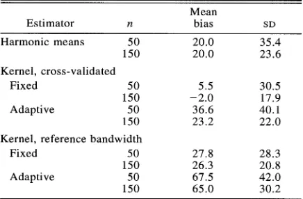
TABLE 3. Percentage bias of estimated areas of complex simulated home ranges, 150 replicates of 15 home range shapes. n = 50 or 150 observations per replicate.

Mean

Estimator n bias SD

Harmonic means 5 0 20.0 35.4 150 20.0 23.6 Kernel, cross-validated

Fixed 50 5.5 30.5 1 50 -2.0 17.9 Adaptive 50 36.6 40.1 150 23.2 22.0 Kernel, reference bandwidth

(7)

FIG.3. Density contours of a complex simulated home range, (A) true density, (B) cross-validated fixed kernel estimate, (C) cross-validated adaptive kernel estimate, (D) h,,, fixed kernel estimate, (E) h,,, adaptive kernel estimate, (F) harmonic mean estimate. Contours represent 95, 72.5, 50, 27.5, and 5% of the volume of the home range estimate; data points mark observation locations.

Pisgah Bear Sanctuary, Pisgah National Forest, North Carolina (Powell 1987, Horner and Powell 1990, Pow-ell et al. 1996).

Data sets for bears that were radio tracked from 1981 through 1990 were submitted to the kernel density estimator for cross validation. Telemetry observations at winter den sites were excluded from this analysis. There were 59.5 2 28.7 observations per home range estimate (mean i 1 SD). Output consisted of the estimated contours of home ranges, the bandwidths (both h,,, and h,,), and the ratio between the cross-validated bandwidth choice and the reference bandwidth choice.

The true size and shape of these ranges is not known, so the performance of the estimator could not be analyzed in this context.

Simulated data: two-ellipse home range

(8)

October 1996 ACCURACY O F KERNEL DENSITY ESTIMATORS

1

A

501

" 1 2 3 4 5 6 7 8 9 10 11 1 2 1 3 1 4 1 5

HOME RANGE

TABLE4. Mean integrated squared error (MISE) for kernel methods. Means are of 2250 replicates (15 home range shapes with 150 replicates each); n = 50 or 150 observa-tions per replicate.

Error

Estimator n Mean SD

LSCVt fixed 50 1.4

x

lo5 4.3

x

lo6 LSCV adaptive 50 6.2 X loz7 2.9 X lozy

h,,, fixed 50 2.8 X loy 9.9 X 1Ol0

h,,, adaptive 50 1.9 X loM 6.5 X

LSCV fixed 150 2.0 X lo3 8.8 X lo4 LSCV adaptive 150 1.4 X l o i y 6.5 X loZ0

h,,, fixed 150 6.3

x

lo5 1.8

x

lo7

h,,, adaptive 150 2.4

x

lo46 1 . 1

x

lo4a

t

LSCV = least squares cross validation.

HOME RANGE

FIG. 4. Mean bias of 150 replicates for each of 15 true home range shapes, estimated by (A) cross-validated fixed kernel, (B) cross-validated adaptive kernel, (C) h,,, fixed kernel, ( D ) h,,,

adaptive kernel, (E) harmonic mean.

TABLE5. Results of least squares cross validation (LSCV) kernel estimation on five black bear home ranges.

H HR

Bcar Year n t ratio$ sizes h,,,, h,,,,'J

Number of radio telemetry locations in the home range.

hcv/hrer

§ Estimated home range size (km2).

11

The LSCV bandwidth (km) for the x axis that was used for this estimate.

(9)

FIG.5 . Telemetry locations with fixed (A, C , E, G, I) and adaptive (B, D, F, H, J) kernel contours for five black bear home ranges: bear 106 (A, B); bear 70 (C, D); bear 163 (E, F); bear 72 (G, H); bear 61 (I, J). Contours and symbols are as in Fig. 3. Axis values are truncated UTM coordinates (km).

estimates of the home range size. Although Boulanger and White (1990) used 1000 replicates, we judged 100 replicates to be adequate since means and standard deviations stabilized with far fewer than this number of replicates (Fig. 2).

Simulated data: complex mixtures

The results of the estimation procedures are illus- trated graphically with one simulated home range (Fig. 3). The parameters of the 10 normal distributions that comprise this home range were presented earlier (Table 1). The numerical results for all replicates follow (Table 3). The cross-validated fixed (Fig. 3B) and adaptive

kernel (Fig. 3C) methods closely estimated the true distribution (Fig. 3A) from which home ranges were simulated, and produced smooth density estimates that show no influence of the evaluation grid. The harmonic mean (Fig. 3F) shows very irregular contours and local minima that result from observations' falling particularly close to evaluation points.

(10)

FIG.5.

sumption of standard normal data (i.e., the reference choice) the density estimate was oversmoothed and re- sulted in a large positive bias in home range size. The harmonic mean had a larger positive bias for these complex home range simulations than did the cross- validated fixed kernel estimates; its standard deviation was approximately the same as those of the cross validated kernel estimators. The accuracy of each estimator varied from one home range shape to another (Fig. 4).

The differences in mean integrated squared error between the various kernel methods were quite large (Ta- ble 4). The cross-validated fixed kernel had the lowest MISE, the adaptive estimates had extraordinarily high MISE.

Real data

Results from five black bears illustrate a range of cross-validated kernel estimates (Table 5, Fig. 5). The contours show the multimodal and often disjunct nature of the home ranges that is typical for these bears, even when sample sizes are large. The adaptive estimates show the contracted inner contours and expanded outer contours that result from this method. Since the true home range cannot be known for free-ranging animals, there is no way to determine the accuracy of these estimates.

Continued.

The kernel method with cross validation produced the most accurate estimates of simulated home ranges. When performing density estimates on data that are multimodal and non-normal, the cross-validated fixed kernel appears to be the best method to use. This cor- roborates Worton's (1995) conclusion that the fixed kernel gives the least biased results, and that proper selection of the smoothing parameter is very important. Although we agree with Worton's (1995) conclusion that the appropriate level of smoothing is the most important factor for obtaining accurate home range size estimates, we make a contrasting conclusion that the choice of whether to use fixed or adaptive kernel density estimation is also important.

We found that the fixed kernel performed better than the harmonic mean estimator that Boulanger and White (1990) found to be the best of the well-known home range estimators. Although they reported a lower bias than we d o for the harmonic mean estimator with the two ellipse simulations, their bias estimate was incor- rect due to their miscalculation of the true area of the simulated distribution.

(11)

width, he apparently used the h,,, bandwidth. Thus, our results for the h,,, bandwidth would substantially agree with his conclusions.

It is interesting that the fixed kernel performed better than the adaptive kernel in all of the tests. Adaptive kernels have been expected to produce better estimates than fixed kernels (Silverman 1986: 110); however, their properties have not been thoroughly explored by statisticians, nor have they been widely applied to real data. This finding is particularly significant for some readily available computer applications of kernel estimation, which primarily provide the adaptive kernel estimate as output. It is possible that implementing the cross validation equation designed for the adaptive kernel (Silverman 1986:106) would improve the adaptive estimates, but this is hard to justify in view of the excellent results of the fixed kernel and the mathematical difficulties with implementing the adaptive cross validation.

Choosing the smoothing parameter by fine-grained least squares cross validation was essential for obtaining accurate estimates. Many of the currently available kernel home range programs do not provide such cross validation. In addition, it is important to collect location data with high precision because LSCV performs quite badly with data that are rounded (i.e., collected on a coarse grid; Silverman 1986, Chiu 1991).

The differences in mean integrated squared error for the different kernel methods were very large, and were strikingly different from the expectation that the adaptive kernel would be the most accurate. Worton (1989b) found lower MISE for adaptive kernels than for fixed kernels tested on bivariate normal data. H e measured MISE at the observations themselves, whereas we measured it at the grid points. Apparently, adaptive kernels give the best density estimate at the actual observation locations, whereas fixed kernels give the best overall surface estimate.

The implementation of any home range estimator will have an important effect on the results. The definition of the harmonic mean home range we used (in- clude all grid points with harmonic mean values that are lower than the highest harmonic mean value at an observation, Ackerman et al. 1990) will make the area estimate highly sensitive to outlying observations. An outlying observation will have a high harmonic mean value, and thus will force the inclusion of many grid points. While it is possible to modify the definition and the methodology of the harmonic mean estimator to improve its accuracy, the necessity of doing so em- phasizes the artificial and inappropriate nature of the harmonic mean as a home range estimator. In contrast, kernel estimators are well defined and tractable.

We attempted to create simulations that would represent reasonable animal home ranges. Nevertheless, the simulated distributions we tested are not actual home ranges, and the results are not strictly indicative

of how the estimators will perform on actual distributions.

The kernel estimates of the black bear home ranges reveal a range of shapes, sizes, and degrees of smoothing. The amount of smoothing varies with the structural irregularity of the data. We feel that the estimates are reasonable representations of these animals' home ranges.

Our simulations were performed with 5 0 and 150 observations per replicate; animal home range studies frequently obtain far fewer than 150 observations per animal. Kernel-based estimates from small samples will be poor at identifying fine structure and will over- estimate home range size. This contrasts with other home range estimation techniques (e.g., minimum con- vex polygon) that show a positive correlation between sample size and home range size (Gautestad and Mys- terud 1993). The more a home range deviates from a smooth unimodal distribution, the larger sample size it will require for accurate estimates.

The fact that the sample size and the data structure affect the degree of smoothing can result in unexpected patterns for LSCV kernel-based estimates of seasonal vs. yearly home ranges. Adding tightly spaced observations (e.g., breeding season observations for a nest- ing animal) to a group of more dispersed (e.g., nonbreeding season) observations can lead to a smaller estimate for the annual home range than for the nonbreeding season home range. This is because the added data from the breeding season causes LSCV to reduce the amount of smoothing compared to that for the nonbreeding data alone. This effect can be prevented in our program by specifying the same value for the annual smoothing parameter as for the nonbreeding season, if desired.

We are most grateful to B. Silverman and D. Nychka for explanations of the kernel estimation procedure. C. Brownie provided suggestions for improving the simulations, J. Bald- win provided explanations of the harmonic mean estimator and comments on a draft of this manuscript. We are especially grateful to B. Worton for a particularly thorough review. Two anonymous reviewers provided valuable comments on a previous draft.

Ackerman, B. B., F. A. Leban, E. 0 . Garton, and M. D. Samuel. 1990. User's manual for program home range. Second edition. Technical Report 15, Forestry, Wildlife and Range Experiment Station. University of Idaho, Moscow, Idaho, USA.

Boulanger, J. G., and G. C. White. 1990. A comparison of home-range estimators using Monte Carlo simulation. Jour- nal of Wildlife Management 54:310-315.

Bowman, A. W. 1985. A comparative study of some kernel- based nonparametric density estimators. Journal of Statis- tical Computing and Simulation 21:313-327.

Breiman, L., W. Meisel, and E. Purcell. 1977. Variable kernel estimates of multivariate densities. Technometrics

19:135-144.

(12)

2085

October 1996 A C C U R A C Y O F K E R N E L DENSITY ESTIMATORS

Calhoun, J. B., and J. U. Casby. 1958. Public Health Mono-

graph Number 55. U.S. Government Printing Office, Wash-

ington, D.C., USA.

Chiu, S. T. 1991. The effect of discretization error on band-

width selection for kernel density estimation. Biometrika

78:436-441.

Dixon, K. R., and J. A. Chapman. 1980. Harmonic mean measure of animal activity areas. Ecology 61:1040-1044.

Epanechnikov, V. A. 1969. Nonparametric estimation of a

multidimensional probability density. Theoretical Proba- bility Applications 14: 153-158.

Fryer, M. J. 1977. A review of some non-parametric methods

of density estimation. Journal of the Institute of Mathe- matics Applications 20:335-354.

Gautestad, A. O., and I. Mysterud. 1993. Physical and bi- ological mechanisms in animal movement processes. Jour- nal of Applied Ecology 30:523-535.

Hayne, D. W. 1949. Calculation of size of home range. Jour-

nal of Mammalogy 30:l-18.

Horner, M. A,, and R. A. Powell. 1990. Internal structure of

home ranges of black bears and analyses of home range overlap. Journal of Mammalogy 71:402-410.

Jennrich, R. I., and F. B. Turner. 1969. Measurement of non- circular home range. Journal of Theoretical Biology 22: 227-237.

Loehle, C. 1990. Home range: a fractal approach. Landscape

Ecology 5:39-52.

Naef-Daenzer, B. 1993. A new transmitter for small animals

and enhanced methods of home-range analysis. Journal of Wildlife Management 57:680-689.

Powell, R. A. 1987. Black bear home range overlap in North

Carolina and the concept of home range applied to black

bears. International Conference on Bear Research and Man- agement 7:235-242.

Powell, R. A., J. W. Zimmerman, D. E. Seaman, and J. F. Gilliam. 1996. Demographic analyses of a hunted black

bear population with access to a refuge. Conservation Bi- ology 10:224-234.

Press, W. H., B. P. Flannery, S . A. Teukolsky, and W. T. Vetterling. 1986. Numerical recipes. Cambridge Univer-

sity Press, Cambridge, UK.

Silverman, B. W. 1986. Density estimation for statistics and

data analysis. Chapman and Hall, London, UK.

Smith, A. T., and E S . Dobson. 1994. A technique for eval-

uation of spatial data using asymmetrical weighted overlap values. Animal Behavior 48: 1285-1292.

Swihart, R. K., and N. A. Slade. 1985. Influence of sampling interval on estimates of home range size. Journal of Wild- life Management 49: 10 19-1025.

Van Winkle, W. 1975. Comparison of several probabilistic

home-range models. Journal of Wildlife Management 39: 118-123.

White, G. C., and R. A. Garrott. 1990. Analysis of wildlife radio-tracking data. Academic Press, San Diego, Califor- nia, USA.

Worton, B. J. 1987. A review of models of home range for

animal movement. Ecological Modelling 38:277-298.

. 1989a. Kernel methods for estimating the utilization

distribution in home-range studies. Ecology 70:164-168.

. 1989b. Optimal smoothing parameters for multi-

variate fixed and adaptive kernel methods. Journal of Sta- tistical Computing and Simulation 32:45-57.

. 1995. Using Monte Carlo simulation to evaluate

(13)

You have printed the following article:

An Evaluation of the Accuracy of Kernel Density Estimators for Home Range Analysis

D. Erran Seaman; Roger A. Powell

Stable URL:

http://links.jstor.org/sici?sici=0012-9658%28199610%2977%3A7%3C2075%3AAEOTAO%3E2.0.CO%3B2-%23

This article references the following linked citations. If you are trying to access articles from an

off-campus location, you may be required to first logon via your library web site to access JSTOR. Please

visit your library's website or contact a librarian to learn about options for remote access to JSTOR.

Literature Cited

Variable Kernel Estimates of Multivariate Densities

Leo Breiman; William Meisel; Edward Purcell

Technometrics, Vol. 19, No. 2. (May, 1977), pp. 135-144.

Stable URL:

http://links.jstor.org/sici?sici=0040-1706%28197705%2919%3A2%3C135%3AVKEOMD%3E2.0.CO%3B2-4

Territoriality and Home Range Concepts as Applied to Mammals

William Henry Burt

Journal of Mammalogy, Vol. 24, No. 3. (Aug., 1943), pp. 346-352.

Stable URL:

http://links.jstor.org/sici?sici=0022-2372%28194308%2924%3A3%3C346%3ATAHRCA%3E2.0.CO%3B2-O

The Effect of Discretization Error on Bandwidth Selection for Kernel Density Estimation

Shean-Tsong Chiu

Biometrika, Vol. 78, No. 2. (Jun., 1991), pp. 436-441.

Stable URL:

http://links.jstor.org/sici?sici=0006-3444%28199106%2978%3A2%3C436%3ATEODEO%3E2.0.CO%3B2-O

Harmonic Mean Measure of Animal Activity Areas

Kenneth R. Dixon; Joseph A. Chapman

Stable URL:

http://links.jstor.org/sici?sici=0012-9658%28198010%2961%3A5%3C1040%3AHMMOAA%3E2.0.CO%3B2-4

http://www.jstor.org

LINKED CITATIONS

(14)

-Physical and Biological Mechanisms in Animal Movement Processes

Arild O. Gautestad; Ivar Mysterud

The Journal of Applied Ecology, Vol. 30, No. 3. (1993), pp. 523-535.

Stable URL:

http://links.jstor.org/sici?sici=0021-8901%281993%2930%3A3%3C523%3APABMIA%3E2.0.CO%3B2-Y

Calculation of Size of Home Range

Don W. Hayne

Journal of Mammalogy, Vol. 30, No. 1. (Feb., 1949), pp. 1-18.

Stable URL:

http://links.jstor.org/sici?sici=0022-2372%28194902%2930%3A1%3C1%3ACOSOHR%3E2.0.CO%3B2-1

Internal Structure of Home Ranges of Black Bears and Analyses of Home-Range Overlap

Margaret A. Horner; Roger A. Powell

Journal of Mammalogy, Vol. 71, No. 3. (Aug., 1990), pp. 402-410.

Stable URL:

http://links.jstor.org/sici?sici=0022-2372%28199008%2971%3A3%3C402%3AISOHRO%3E2.0.CO%3B2-S

Demographic Analyses of a Hunted Black Bear Population with Access to a Refuge

Roger A. Powell; John W. Zimmerman; D. Erran Seaman; James F. Gilliam

Conservation Biology, Vol. 10, No. 1. (Feb., 1996), pp. 224-234.

Stable URL:

http://links.jstor.org/sici?sici=0888-8892%28199602%2910%3A1%3C224%3ADAOAHB%3E2.0.CO%3B2-L

Kernel Methods for Estimating the Utilization Distribution in Home-Range Studies

B. J. Worton

Ecology, Vol. 70, No. 1. (Feb., 1989), pp. 164-168.

Stable URL:

http://links.jstor.org/sici?sici=0012-9658%28198902%2970%3A1%3C164%3AKMFETU%3E2.0.CO%3B2-Y

http://www.jstor.org