Predictive data mining based on similarity and clustering methods.

(1)

PREDICTIVE DATA MINING BASED ON

SIMILARITY AND CLUSTERING METHODS

Sarjon Defit, Mohd Noor Md Sap

Faculty of Computer Science and Information System University Technology of Malaysia, KB. 791

80990 Johor Bahru, Malaysia Telp: (607)-5576160, Fax: (607) 5566155 {[email protected]},{ [email protected]}

Abstract

Predictive data mining is an attractive goal in data mining. It has wide application, including credit evaluation, sales promotion, financial forecasting and market trend analysis. In this paper we propose a predictive data mining model based on the combination of similarity, clustering and predictive modeling. This model is implemented and tested using real estate data. Our study concludes that our predictive data mining model can improve the prediction ability by using all attributes in the different clusters with the nearest distance as input fields. In this paper we explain the importance of data mining, similarity, the proposed predictive data mining model, the testing of the model, discussion and conclusion.

Keywords: Data Mining, Predictive Data Mining, Similarity, Clustering, Predictive Modeling

1. Introduction

With the development of high capacity storage technology, a large amount of data can be stored. The data stored in databases consists of simple information, text document, or complex information such as multimedia, spatial databases, and hypertext documents (Tung, L., Kyung, K., 1997: Olaru,

c.,

Wehenkel, L., 1999; Zaiane, R., 1999; Sarjon, D., Mohd, N., 2000). The stored data carry numerous valuable knowledge that can be extracted using many available tools such as SQL (Structure Query Language) and QBE (Query By Example). Generally these techniques can only extract the meaning of data. We need a technique that can be used to extract not only the meaning but also the knowledge from the large amount of data. One of the tools is data mining. The result of the extracted knowledge can be applied to information management, query processing, decision process, process control and many other applications (Yongjian, 1996; Sarjon, D., Mohd, N., 2000)

(2)

56

There are many definitions of data mining taken from different views. Jiawei, H. et.al (Jiawei, H., Chiang, Y. et.al., 1997) give the definition data mining as the discovery of knowledge and useful information from the large amounts of data stored in databases and Olaru, C. et.al (Olaru, C; Wehenkel,L., 1999) define data mining as the non trivial process of extracting valid, previously unknown, comprehensible and useful information from large databases. McLauren (McLauren,I., 1997) defines data mining as the automatic extraction of non trivial potentially useful, patterns from large databases, while Sheng-Chai, C. et.al (Sheng-Chai, C., Hung-Pin, C. et.al. 1999) defines data mining as the process of extracting valid, previously unknown information from large databases and using it to make crucial business decision. Last, Goebel, M et.al (Goebel, M., Le, G., 1999) define data mining as the extraction of patterns or models from observed value. From the above definitions, we concludes that data mining is the automatic extraction of patterns, previously unknown and potentially useful information from large amount of data in databases and using it to make crucial business decision.

Data Mining is divided into two main categories, namely, descriptive and predictive data mining (Jiawei, H., 1999; Olaru,

c.,

Wehenkel,L., 1999; Zaiane, R., 1999, Sarjon, D., Mohd, N., 2000). The function of descriptive data mining is to describe the general properties of existing data, and to create meaningful subgroups such as demographic cluster. Compared to descriptive data mining, predictive data mining is used to forecast explicit value based on inference on available data.

Predictive data mining is a major task in data mmmg and has a wide application, including credit evaluation, sales promotion, financial forecasting and market trend analysis (Shan, C; 1998; Wei, W., 1999). Many predictive data mining algorithms have been developed in the past research. For example, (Shan,

c.,

1998) proposed predictive data mining method which consists of three steps, namely data generalization, relevance analysis and statistical regression model. In the middle of 1999, (Wei, W., 1999) proposed two predictive data mining methods. The first method is a classification-based method which integrates Attribute Oriented Induction (AOI) with the ID3 decision tree method. The second method is a pattern matching-based method which integrates statistical analysis with Attribute Oriented Induction to predict data values of the attribute of interest based on similar groups of data in databases. These predictive data mining methods provide high prediction quality and it leads to efficient and interactive prediction in large databases. However, these methods still encounter several weaknesses and need further improvement. Some of the weaknesses are as follow:

a. These methods did not pursue a best subset of similarity attributes for prediction (Shan,

c.,

1998)

(3)

b. These methods did not apply special data preprocessing techniques to identify which of data in databases are inaccurate, irrelevant or missing value (Shan,

c.,

1998; Wei, W.,

1999).

Looking at the above mentioned weaknesses, we are interested to overcome the first weakness.

The rest of the paper is organized as follow. Section 2 explains the importance of similarity. The proposed predictive data mining model is given in section 3 and testing of the model in section 4. The results of the experiment and conclusion are given in section 5 and 6.

2. Similarity

Similarity is a measure of similar or dissimilar between two or more attributes in the databases (Everitt, S., 1993; Ronkainen, P., 1998). This is one of the central concepts in data mining and knowledge discovery (Ronkainen, P., 1998; Shan, C., 1998; Wei, W., 1999). In searching patterns and regularities, it is not enough to consider only the equality or inequality of data. Instead, we have to consider how the similarity between two or more attributes (Ronkainen, P., 1998; Balasubramanian, S., Hermann, J. W., 1999).

Ronkainen, P. (Ronkainen, P.,1998) proposed two similarity methods, internal and external measure of similarity. The internal measure of similarity is used to measure the similarity between two attributes, while external measure of similarity is used to measure the similarity between more than two attributes. In this paper, we will use the internal measure of similarity.

The similarity between attributes is needed in some databases and knowledge discovery applications. Some examples of such applications are given in the following:

i) Real estate data contains valuable information about the indicators that affects the movement of the house price. Information about indicator with similar effect pattern can be useful in predicting the house prices.

ii) In financial market data, finding stocks that had last week pnce fluctuation from financial time series data, or identifying companies whose stock price have similar pattern growth.

These examples describe how important and essential the notion of similarity for data mining. Searching for similarity attributes can help the prediction, hypothesis testing and

(4)

58

discovery rules. It is not feasible to use all the attributes in databases to do prediction. In most cases, a few of these attributes are highly similar and valuable for prediction. Thus, the effective similarity is necessary to filter out those attributes which are similar or dissimilar.

The meaning of similarity depends on what kind of similarity we are looking for. Using the different similarity measure can determine two attributes to be very similar by one measure and very different by another. This means that we have to carefully choose one particular measure, or we have to try several measure on the data and then choose the one that suits best our purposes (Ronkainen, P., 1998; Shan, C., 1998).

There is no single definition for similarity. In this paper, we define the similarity between attributes is a complementary notion of distance. A measure d for distance between two attributes should be a metric. There are four standard criteria that can be used to determine whether a similarity measure is a true metric or not (Aldenderfer, S., Blashfield, K., 1984, Everitt,S., 1993; Ronkainen, P., 1998). These are:

i) Symmetry. Given two entities, x and y, the distance, d,. Between them satisfies the expression:

(x.y) d

=

d(y,x) ~

°

(I)

ii) Triangle inequality. Given three entities, x.y.z, the distances between them satisifies the expression

d(x,y)~d(x,z)+d(y,z)

iii) Distinguishability of nonidenticals. Given two entities x and y, If d(x,y) -t:. 0, then x-t:. y

iv) Indistinguishability of identicals. For two identical elements, x and x', d(x,x')

=

°

3. The Predictive Data Mining Model

(2)

(3)

(4)

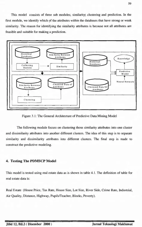
At the present stage we propose a predictive data mining based on the combination of similarity, clustering and predictive modeling (PDMSCP). The general architecture is shown in figure 3.1.

(5)

This model consists of three sub modules; similarity, clustering and prediction. In the

first module, we identify which of the attributes within the databases that have strong or weak

similarity. The reason for identifying the similarity attributes is because not all attributes are

feasible and suitable for making a prediction.

1

Clustered Data of Attributes

Historical Databases

Neural Network

C lu sterin g f···

Figure 3.1:The General Architecture of Predictive Data Mining Model

The following module focuss on clustering those similarity attributes into one cluster

and dissimilarity attributes into another different clusters. The idea of this step is to separate

similarity and dissimilarity attributes into different clusters. The final step is made to

construct the predictive modeling.

4. Testing The PDMSCP Model

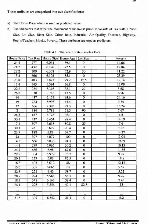
This model is tested using real estate data as is shown in table 4.1. The definition of table for

real estate data is:

Real Estate (House Price, Tax Rate, House Size, Lot Size, River Side, Crime Rate, Industrial,

Air Quality, Distance, Highway, Pupils/Teacher, Blocks, Poverty).

(6)

60

These attributes are categorized into two classifications;

a) The House Price which is used as predicted value.

b) The indicators that affect the movement of the house price. It consists of Tax Rate, House Size, Lot Size, River Side, Crime Rate, Industrial, Air Quality, Distance, Highway, Pupils/Teacher, Blocks, Poverty. These attributes are used as predictors.

Table 4.1 : The Real Estate Samples Data

House Price Tax Rate House Size House Age Lot Size ... Poverty

24.4 277 6.064 59.1 0 14.66

21.2 432 6.176 72.5 0 12.04

22.2 300 6.358 52.9 30 11.22

13.4 666 6.103 85.1 0 23.29

23.8 403 5.877 79.2 12.5 12.14

17.4 345 5.594 36.8 0 13.09

22.2 224 6.316 38.1 22 5.68

26.2 330 6.718 17.5 0 6.56

14 437 6.174 93.6 0 24.16

19 224 5.995 45.4 0 9.74

17 666 7.393 99.3 0 16.74

8 384 6.781 71.3 90 7.67

26.5 187 6.728 36.1 0 4.5

30.1 437 6.454 98.4 0 14.59

17.1 307 6.618 80.8 25 7.6

30.1 281 6.619 70.4 0 7.22

23.9 188 5.87 69.7 0 14.37

22 307 6.072 100 0 13.04

14.5 666 6.833 94.3 0 19.69

14.1 279 5.966 30.2 0 10.13

24.7 666 6.98 67.6 0 11.66

29.8 304 5.972 76.7 0 9.97

20.3 233 6.03 85.5 0 18.8

16.6 403 5.012 88 0 12.12

15.3 305 6.065 7.8 0 5.52

22.8 222 6.43 58.7 0 5.21

28.7 224 5.968 58.5 0 9.29

18.7 348 6.162 38.4 0 7.43

24.1 223 5.856 42.1 82.5 13

...

... ... '" ... ...

.

..

... ... ... ...

.

.. ...

.

..

31.5 307 6.552 21.4 0 6.2

(7)

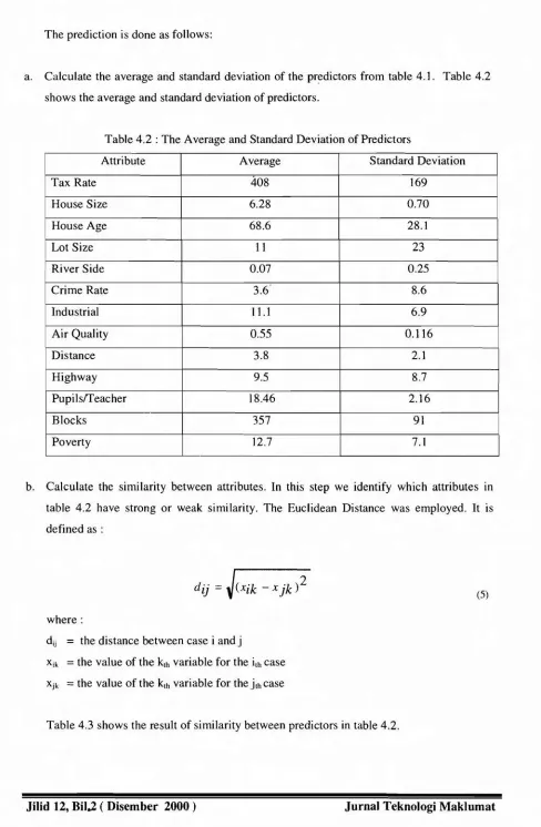
The prediction is done as follows:

a. Calculate the average and standard deviation of the predictors from table 4.1. Table 4.2 shows the average and standard deviation of predictors.

Table 4.2 : The Average and Standard Deviation of Predictors

Attribute Average Standard Deviation

Tax Rate 408 169

House Size 6.28 0.70

House Age 68.6 28.1

Lot Size 11 23

River Side 0.07 0.25

Crime Rate 3.6 8.6

Industrial 11.1 6.9

Air Quality 0.55 0.116

Distance 3.8 2.1

Highway 9.5 8.7

Pupils/Teacher 18.46 2.16

Blocks 357 91

Poverty 12.7 7.1

b. Calculate the similarity between attributes. In this step we identify which attributes in table 4.2 have strong or weak similarity. The Euclidean Distance was employed. It is defined as:

where:

dij

=

the distance between case i andj

Xik

=

the value of the k_th variable for the i_lhcase Xjk

=

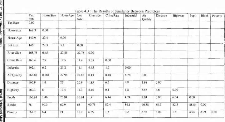
the value of the kthvariable for thejthcase

Table 4.3 shows the result of similarity between predictors in table 4.2.

(5)

(8)

~

...

-s:

_....

J'J

=

...

~

..--e

...

til /'C)

:3

'a' /'C)

..,

N

=

"-' ~

=

..,

=

₌

-""3 /'C) ~

=

e

-e a;9.

s:

~

=

....

Table 4.3 : The Results of Similarity Between Predictors

Tax HouseSize HouseAge Lot Riverside CrimeRate Industrial Air Distance Highway Pupil Block Poverty

Rate Size Quality

Tax Rate 0.00

HouseSize 168.3 0.00

House Age 140.9 27.4 0.00

I I

I

Lot Size 146 22.3 5.1 0.00

River Side 168.75 0.45 27.85 22.75 0.00

Crime Rate 160.4 7.9 19.5 14.4 8.35 0.00

Industrial 162.1 6.2 21.2 16.1 6.65 1.7 0.00

Air Quality 168.88 0.584 27.98 22.88 0.13 8.48 6.78 0.00

Distance 166.9 1.4 26 20.9 1.85 6.5 4.8 1.98 0.00

Highway 160.3 8 19.4 14.3 8.45 0.1 1.8 8.58 6.6 0.00

Pupils 166.84 1.46 25.94 20.84 1.91 6.44 4.74 2.04 0.06 6.54 0.00

Blocks 78 90.3 62.9 68 90.75 82.4 84.1 90.88 88.9 82.3 88.84 0.00

Poverty 161.9 6.4 21 15.9 6.85 1.5 0.2 6.98 5.00 1.6 4.94 83.9 0.00

(9)

c. Clustering the attributes in table 4.3 into clusters based on similarity. We employed the

-single linkage clustering as is given in algorithm 4.1. The inter cluster in this method is

defined as the distance between the closest members of the two clusters.

where :

d(ci, cj) =the inter cluster distance between two singleton cluster ci =(yk) and cj=(yl)

Algorithm 4.1 :The Single Linkage Clustering Algorithm

Start: Cluster C}, C2,.••, Cn. Each containing a single individual.

I. Find nearest pair of distinct cluster, say C, and C; 2. Merge

C

and

c,

3. Delete C,

4. Decrementnumber of cluster by one

5. If number of clusters equal one then stop 6. Else return to I

Table 4.4 shows the result of clustering the predictors in table 4.3.

Table 4.4: The Clustering of Predictors

Number of Cluster Description

Cluster-I {Distance, Pupils}

Cluster-2 { Crime Rate, Highway}

Cluster-3 { River Side, Air Quality}

Cluster-4 { Industrial, Poverty}

Cluster-S {House Size}

Cluster-6 {House Age. Lot Size}

Cluster-7 {Blocks}

Cluster-S {Tax Rate}

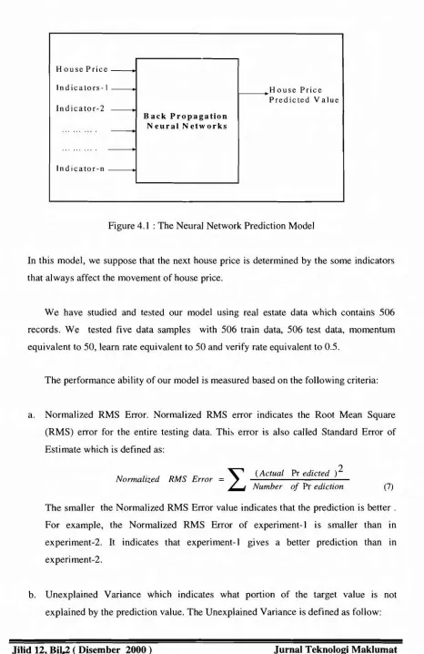
d. Prediction modeling.In this step we employed Back Propagation Neural Network. Figure

4.1 shows the Neural Network Prediction Model.

(10)

64

House Price---.

Indicators-l ---.

Indicator-2 ---.

Back Propagation Neural N etw orks ... ... ... . ---.

lndi c a to r -n - - + I

I---_ _H ouse Price Predicted Value

Figure 4.1 :The Neural Network Prediction Model

In this model, we suppose that the next house price is determined by the some indicators

that always affect the movement of house price.

We have studied and tested our model using real estate data which contains 506

records. We tested five data samples with 506 train data, 506 test data, momentum

equivalent to 50, learn rate equivalent to 50 and verify rate equivalent to 0.5.

The performance ability of our model is measured based on the following criteria:

a. Normalized RMS Error. Normalized RMS error indicates the Root Mean Square

(RMS) error for the entire testing data. This error is also called Standard Error of

Estimate which is defined as:

N I· d RMS E

L

(Actual Pr edicted )

2

ormatze rror =

Number of Pr ediction (7)

The smaller the Normalized RMS Error value indicates that the prediction is better.

For example, the Normalized RMS Error of experiment-l is smaller than In

experiment-2. It indicates that experiment-I gives a better prediction than In

experiment-2.

b. Unexplained Variance which indicates what portion of the target value is not

explained by the prediction value. The Unexplained Variance is defined as follow:

(11)

. (Actual RMS £rror)2

UnexplamedVariance= . . . ; . . . .

-Variance of T arg et Column (8)

The smaller the Unexplained Variance value gives a better prediction. For example, the Unexplained Variance of experiment-3 is smaller than in experiment 4. It indicates that experiment 3 givesa better prediction than in experiment 4.

c. Correlation Coefficient. It is a number between zero and one which indicates how well the prediction is correlated to the actual. A value of one indicates perfect predictions, and a value of zero indicates no relationship between prediction and target. The Correlation Coefficient is defined as follow:

Corr. Coefficiert

=

JO-

Unexplained Variance)

5. The Experimental Results and Discussion

(9)

Inthe following, we demonstrate the results of the experiment on prediction based on table 4.4.

a. Using the attributes in the same cluster as input fields. For example, predict the next house price using attributes in cluster-I. Table 5.1 shows the result of experiment.

Table 5.1: The Result of Experiment

Normalized RMS Error 16.20

Unexplained Variance 0.63

Correlation Coefficient 0.61

(12)

66

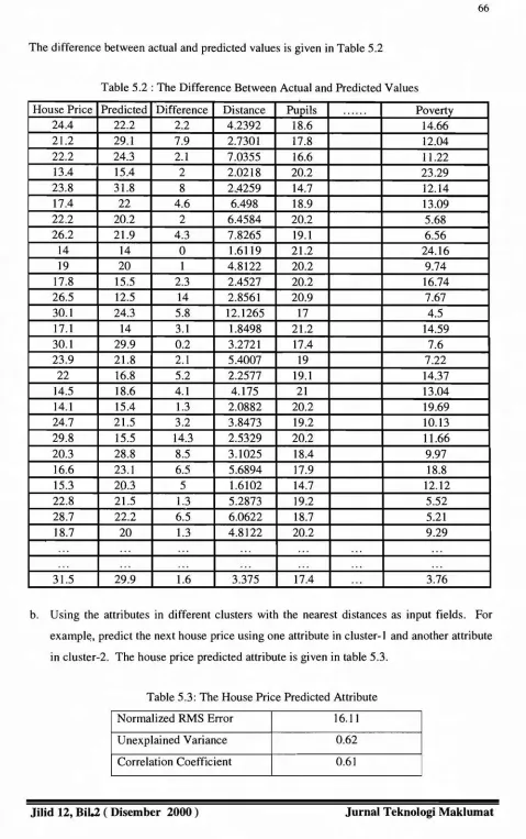
The difference between actual and predicted values is given in Table 5.2

Table 5.2: The Difference Between Actual and Predicted Values

House Price Predicted Difference Distance Pupils ... Poverty

24.4 22.2 2.2 4.2392 18.6 14.66

21.2 29.1 7.9 2.7301 17.8 12.04

22.2 24.3 2.1 7.0355 16.6 11.22

13.4 15.4 2 2.0218 20.2 23.29

23.8 31.8 8 2.:4259 14.7 12.14

17.4 22 4.6 6.498 18.9 13.09

22.2 20.2 2 6.4584 20.2 5.68

26.2 21.9 4.3 7.8265 19.1 6.56

14 14 0 1.6119 21.2 24.16

19 20 1 4.8122 20.2 9.74

17.8 15.5 2.3 2.4527 20.2 16.74

26.5 12.5 14 2.8561 20.9 7.67

30.1 24.3 5.8 12.1265 17 4.5

17.1 14 3.1 1.8498 21.2 14.59

30.1 29.9 0.2 3.2721 17.4 7.6

23.9 21.8 2.1 5.4007 19 7.22

22 16.8 5.2 2.2577 19.1 14.37

14.5 18.6 4.1 4.175 21 13.04

14.1 15.4 1.3 2.0882 20.2 19.69

24.7 21.5 3.2 3.8473 19.2 10.13

29.8 15.5 14.3 2.5329 20.2 11.66

20.3 28.8 8.5 3.1025 18.4 9.97

16.6 23.1 6.5 5.6894 17.9 18.8

15.3 20.3 5 1.6102 14.7 12.12

22.8 21.5 1.3 5.2873 19.2 5.52

28.7 22.2 6.5 6.0622 18.7 5.21

18.7 20 1.3 4.8122 20.2 9.29

...

31.5 29.9 1.6 3.375 17.4 ... 3.76

b. Using the attributes in different clusters with the nearest distances as input fields. For

example, predict the next house price using one attribute in cluster-l and another attribute

in cluster-2. The house price predicted attribute is given in table 5.3.

Table 5.3: The House Price Predicted Attribute

(13)

Table 5.4 shows the difference between actual and predicted values.

Table 5.4 : The Difference Between Actual and Predicted Values

House Price Predicted Difference Crime Rate PUpils ... Poverty 24.4 22.7 1.7 0.13587 18.6 14.66 21.2 23.4 2.2 0.13158 17.8 12.04 22.2 24 1.8 0.1029 16.6 11.22 13.4 17.5 4.1 7.05042 20.2 23.29 23.8 21.7 2.1 1.80028 14.7 12.14 17.4 22.3 4.9 0.13554 18.9 13.09 22.2 19.7 2.5 0.05083 20.2 5.68 26.2 22 4.2 0.19073 19.1 6.56 14 16.3 2.3 0.2909 21.2 24.16 19 19.7 0.7 0.054497 20.2 9.74 17.8 14.8 3 8.24809 20.2 16.74 26.5 17.5 9 0.11432 20.9 7.67 30.1 23.9 6.2 0.01709 17 4.5 17.1 16.3 0.8 0.35233 21.2 14.59 30.1 23.7 6.4 0.6147 17.4 7.6 23.9 22.1 1.8 0.04462 19 7.22

22 22 0 0.06899 19.1 14.37

I 14.5 17 2.5 1.35472 21 13.04

14.1 12.5 1.6 lb.0623 20.2 19.69 24.7 21.8 2.9 0.17505 19.2 10.13 29.8 19.3 10.5 4.64689 20.2 11.66 20.3 22.9 2.6 0.3494 18.4 9.97 16.6 23.3 6.7 0.22927 17.9 18.8 15.3 26.3 11 1.12658 14.7 12.12 22.8 21.8 1 0.09164 19.2 5.52 28.7 22.6 6.1 0.02985 18.7 5.21 18.7 19.7 1 0.06151 20.2 9.29

...

.. .

...

' " ' "

...

.

..

.. .

.31.5 23.7 7.8 0.44178 17.4

...

3.76

c. Using the attributes in different clusters with the furthest distances as input fields. For

example, predict the next house price using one attribute in cluster-I and another attribute

in cluster-8. Table 5.5 shows the house price predicted attribute.

(14)

68

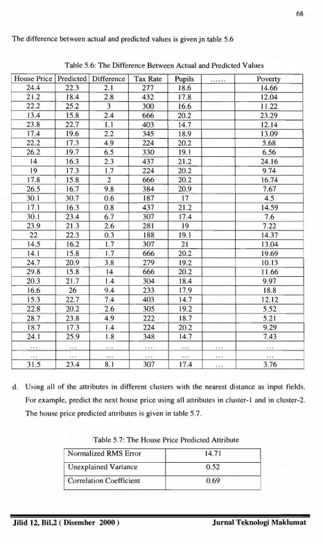
The difference between actual and predicted values is given jn table 5.6

House Price Predicted Difference Tax Rate Pupils ... Poverty

24.4 22.3 2.1 277 18.6 14.66

21.2 18.4 2.8 432 17.8 12.04

22.2 25.2 3 300 16.6 11.22

13.4 15.8 2.4 666 20.2 23.29

23.8 22.7 1.1 403 14.7 12.14

17.4 19.6 2.2 345 18.9 13.09

22.2 17.3 4.9 224 20.2 5.68

26.2 19.7 6.5 330 19.1 6.56

14 16.3 2.3 437 21.2 24.16

19 17.3 1.7 224 20.2 9.74

17.8 15.8 2 666 20.2 16.74

26.5 16.7 9.8 384 20.9 7.67

30.1 30.7 0.6 187 17 4.5

17.1 16.3 0.8 437 21.2 14.59

30.1 23.4 6.7 307 17.4 7.6

23.9 21.3 2.6 281 19 7.22

22 22.3 0.3 188 19.1 14.37

]4.5 16.2 1.7 307 21 13.04

14.1 15.8 1.7 666 20.2 19.69

24.7 20.9 3.8 279 19.2 10.13

29.8 15.8 14 666 20.2 11.66

20.3 21.7 1.4 304 18.4 9.97

16.6 26 9.4 233 17.9 18.8

15.3 22.7 7.4 403 14.7 12.12

22.8 20.2 2.6 305 19.2 5.52

28.7 23.8 4.9 222 18.7 5.21

18.7 17.3 1.4 224 20.2 9.29

24.1 25.9 1.8 348 14.7 7.43

... ... ...

...

.

.. ... . ..

... ...

...

... ...

31.5 23.4 8.1 307 17.4 ... 3.76

d. Using all of the attributes in different clusters with the nearest distance as input fields.

For example, predict the next house price using all attributes in cluster-I and in cluster-2.

The house price predicted attributes is given in table 5.7.

(15)

Table 5.8 shows the difference between actual and predicted values.

Table 5.8: The Difference Between Actual and Predicted Values House Price Predicted Difference Crime Rate Distance

...

Poverty

24.4 20.9 3.5 0.13587 4.2392 14.66

21.2 27.1 5.9 0.13158 2.7301 12.04

22.2 24.4 2.2 0.1029 7.0355 11.22

13.4 15.1 1.7 7.05042 2.0218 23.29

23.8 32.3 8.5 1.80028 2.4259 12.14

17.4 24.4 7 p.13554 6.498 13.09

22.2 23.4 1.2 0.05083 6.4584 5.68

26.2 24.2 2 0.19073 7.8265 6.56

14 12.2 1.8 0.2909 1.6119 24.16

19 20.7 1.7 0.054497 4.8122 9.74

17.8 14.7 3.1 8.24809 2.4527 16.74

26.5 15.4 11.1 0.11432 2.8561 7.67

30.1 24.4 5.7 0.01709 12.1265 4.5

17.1 15 2.1 0.35233 1.8498 14.59

30.1 32.2 2.1 0.6147 3.2721 7.6

23.9 24.1 0.2 0.04462 5.4007 7.22

22 23.3 1.3 0.06899 2.2577 14.37

14.5 15.3 0.8 1.35472 4.175 13.04

14.1 13.1 1 10.0623 2.0882 19.69

24.7 17.6 7.1 0.17505 3.8473 10.13

29.8 17.3 12.5 4.64689 2.5329 11.66

20.3 26.8 6.5 0.3494 3.1025 9.97

16.6 24.4 7.8 0.22927 5.6894 18.8

15.3 19.2 3.9 1.12658 1.6102 12.12

22.8 23.9 1.1 0.09164 5.2873 5.52

28.7 24.4 4.3 0.02985 6.0622 5.21

18.7 20.7 2 0.06151 4.8122 9.29

24.1 24.5 0.4 0.03445 6.27 7.43

...

.

..

.

.. ' "

...

31.5 32.9 1.4 0.44178 3.375 ... 3.76

e. Using all of the attributes in different clusters with the furthest distances as input fields. For example, predict the next house price using all attributes in cluster-I and in cluster-S. Table 5.9 shows the house price predicted attribute.

(16)

70

The difference between actual and predicted values is given in table 5.10.

House Price Predicted Difference Tax rate Distance ... Poverty

24.4 23.9 0.5 277 4.2392 14.66

21.2 17.5 3.7 432 2.7301 12.04

22.2 19.7 2.5 300 7.0355 11.22

13.4 12.9 0.5 666 2.0218 23.29

23.8 26 2.2 403 2.4259 12.14

17.4 18.4 1 345 6.498 13.09

22.2 21.4 0.8 224 6.4584 5.68

26.2 19.1 7.1 330 7.8265 6.56

14 17.6 3.6 437 1.6119 24.16

19 18.4 0.6 224 4.8122 9.74

17.8 13.9 3.9 666 2.4527 16.74

26.5 17.8 8.7 384 2.8561 7.67

30.1 41.1 11 187 12.1265 4.5

17.1 17.6 0.5 437 1.8498 14.59

30.1 28.2 1.9 307 3.2721 7.6

23.9 26.1 2.2 281 5.4007 7.22

22 20.6 1.4 188 2.2577 14.37

14.5 17.9 3.4 307 4.175 13.04

14.1 13.1 1 '666 2.0882 19.69

24.7 20.1 4.6 279 3.8473 10.13

29.8 14.1 15.7 666 2.5329 11.66

20.3 22 1.7 304 3.1025 9.97

16.6 21.3 4.7 233 5.6894 18.8

15.3 21.1 5.8 403 1.6102 12.12

22.8 25.6 2.8 305 5.2873 5.52

28.7 28.9 0.2 222 6.0622 5.21

18.7 18.4 0.3 224 4.8122 9.29

24.1 27.8 3.7 348 6.27 7.43

... ... ... .., _." ... ...

..,

.

,

.

.,

.

.,. ... ...

.

..

31.5 28.4 3.1 307 3.375 ... 3.76

In the following we illustrate the comparison among the results. Table 5.11 summarizes the

results of Normalized RMS Error, Unexplained Variance and Correlation Coefficient. Graph

5.1 shows the comparison among the results.

(17)

Table 5.11: The Resultsof Normalized RMS Error,Unexplained Variance and Correlation Coefficient

Normalized RMS Unexplained Correlation Error Variance Coefficient Experiment-I 16.20 0.63 0.61

Experiment-2 16.11 0.62 0.61

Experiment-S 16.7 0.68 0.57

Experiment-4 14.71 0.52 0.69

Experiment-5 15.38 0.57 0.66

Graph 5.1:The Comparison Among the Results

t

·

Normalized RMS ErrorI

_ _ Unexplained Variance

.. Correlation Coefficien-.!J

20

15

10

5

o

r--·

-!

l -__.. .. .

The previousresult sof the experiment showsthat :

a) Using all attributes in different clusters with the furthest distances as input field gives a better prediction. The prediction has Normalized RMS Error equivalent to 14.71, Unexplained Variance equivalent to 0.52 and Correlation Coefficient equivalent to 0.69 Using the similarity techniquewe can pursue the best subset of similarity attributes to do prediction. This means that the combination of distance, pupils, crime rate and highway attributesas predictors in real estate data can improve the prediction ability.

(18)

72

6. Conclusion

Similarity is one of the important techniques in predictive data mining. Not all attributes

within databases are feasible and suitable to do prediction. Therefore, we need to identify

which of the attributes that have strong or weak similarity. At the present stage, we propose a

predictive data mining model based on similarity method which consists of three main steps,

similarity, clustering and predictive modeling. This model has been implemented and tested

using real estate data. The result of the experiment shows that:

a) Using all attributes in different clusters with the nearest distances as input fields could

give a better prediction.

b) Using similarity technique can improve the ability of making a prediction.

(19)

References

Aldenderfer, S., Blashfield,K. (1984). "Cluster Analysis", Stage Publication

Balasubramanian, S., Hermann, J. W., (1999). "Using Neural Networks to Generate Design Similarity Measures".

Everitt, S. (1993). "Cluster Analysis", Third Edition, New York, Halsted Press

Goebel, M., Le, G. (1999). " A Survey of Data Mining and Knowledge", SIGKDD Exploration Volume I, Issue I, Page 20-23

Jiawei, H. (1999). "Characteristic Rules"; In W. Kloesgen and J. Zytkow (eds). Handbook of Data Mining and Knowledge Discovery, Oxford University Press, 1999

Jiawei, H., Chiang, Y. et.al, (1997). " DBMiner: A System for Data Mining in Relational Databases and Data Warehouse", Proc. 1996 Int'I Conf. on Data Mining and Knowledge Discovery (KDD'96) Porland, Oregon, August 1996, pp 250-155

McLaren, I., (1997). "Data Mining: Finding Business Value in Data". Available online via URL : http://homelclara.net/imclaran/dmpaper.html

Olaru,

c.,

Wehenkel, L. (1999). "Data Mining". IEEE Computer Application in Power, July 1999

Ronkainen, P. (1998). " Attribute Similarity Event Sequence Similarity in Data Mining", Ph. Lie Thesis, Report C-1998-42, University of Helsinki, Department of Computer Science, October 1998

Sarjon, D., Mohd, N. (2000

). " Data Mining: A Preview", Journal of Information Technology", Jilid 12, Bil I, Jun 2000,. page 57-84

Shan,

c.,

(1998). " Statistical Approach to Predictive Modeling in Large Databases", MSc Thesis, Computing Science, Simon Fraser University, March 1998

(20)

74

Sheng-Chai, C., Hung-Pin, C. et.a\. (1999). "A Forecasting Approach for Stock Index Future Using Grey Theory and Neural Networks". IEEE, 1999

Tung, L., Kyung, K. (1997). "Data Mining Applications in Singapore". Available online via

URL: http://www.sbanet.uca.edu/DOCS/981csb/q005 .

Wei, W., (1999). " Predictive Modeling Based on Classification and Pattern Matching

Method", MSc Thesis, Computing Science, Simon Fraser University, Augustus 1999

Wuthrich, B., Permunetilleke, P. et.a\. (1998a). "Daily Prediction of Major Stock Indices

From Textual WWW Data".

Wuthrich, B., Permunetilleke, P. et.a\. (l998b. "Daily Stock Market Forecast From Textual

Web Data", IEEE, 1998.

Zaiane, R. (1999). " Introduction to Data Mining". CMPUT690 Principles of Knowledge

Discovery III Databases. Available online via URL

http://www.cs.ualberta.cal-zaiane/courses/cmput690/noteslchapterlIindex .html