An Analysis of Local Out-of-Plane Buckling of Ductile Reinforced Structural Walls Due to In-Plane Loading.

(1)

ABSTRACT

HERRICK, CHRISTOPHER KELLY. An Analysis of Local Out-of-Plane Buckling of Ductile Reinforced Structural Walls Due to In-Plane Loading. (Under direction of Mervyn J. Kowalsky.)

(2)

(3)

An Analysis of Local Out-of-Plane Buckling of Ductile Reinforced Structural Walls Due to In-Plane Loading

by

Christopher Kelly Herrick

A thesis submitted to the Graduate Faculty of North Carolina State University

in partial fulfillment of the requirements for the degree of

Master of Science

Civil Engineering

Raleigh, North Carolina 2014

APPROVED BY:

_______________________________ Mervyn J. Kowalsky

Committee Chair

_______________________________ James M. Nau

(4)

ii DEDICATION

I dedicate this thesis to my better half, Christine Nguyen. Thank you for your boundless assistance, never-ending encouragement and seemingly infinite patience and love that led to this being possible.

(5)

iii BIOGRAPHY

(6)

iv

ACKNOWLEDGMENTS

I would like to thank my graduate advisor Dr. Mervyn Kowalsky for his time, effort and patience throughout my time as a graduate student. I am also grateful to Dr. James Nau, whose endless words of advice and support have guided my educational career to date. Towards Dr. Rudolf Seracino I also extend a special thank you, for being member on my committee and providing me his expertise on reinforced concrete.

I would like to thank Dr. Sri Sritharan for providing many of the pictures within this thesis. I would also like to thank Dr. Murthy Guddati for providing his insight on analytical methods for modeling buckling.

I must also extend my gratitude to my friends at the Constructed Facilities Laboratory: Yuhao Feng, Steven Fulmer, Chad Goodnight, Nicole King, Easa Khan and many others, all of whom who not only put up with my extended, over-complicated structural engineering discussions, thought experiments and “what-if” questions, but also who shared their time, knowledge, and experience with me despite this.

(7)

v

CHAPTER 4. RESEARCH METHODS ... 40

4.1 General Discussion ... 40

4.2 Cumbia ... 40

4.2.1 Variance of Confinement ... 41

4.2.2 Calculation of Longitudinal Steel Reinforcement Ratio ... 43

4.2.3 Calculation of Plastic Hinge Lengths ... 44

4.2.4 Shear Strength ... 45

CHAPTER 5. EXAMINATION OF PRIOR EXPERIMENTAL RESULTS ... 47

(8)

vi

5.2.1 Goodsir [17]... 48

5.2.2 He and Priestley [48] ... 51

5.2.3 Ji [22] ... 54

5.2.4 Jiang [23] ... 56

5.2.5 Lefas and Kotsovos [26][27] ... 58

5.2.6 Oesterle et al. [39][40] ... 60

5.2.7 Zhang [53] ... 62

5.2.8 Zhou [54] ... 63

5.2.9 Comparison of Experimental Results with Predictions ... 65

5.3 Experimental Tests of Prism Specimens... 69

5.3.1 Azimikor et al. [3] ... 69

5.3.2 Chai and Elayer [7] ... 71

5.3.3 Chrysandis and Tegos [9][10] ... 72

5.3.4 Creagh et al. [11] ... 74

5.3.5 Goodsir [17] ... 76

5.3.6 Comparison of Prism Results... 78

5.4 Conclusions from Prior Experimental Testing ... 80

CHAPTER 6. PARAMETRIC STUDIES ... 82

6.2 Parametric Study: Phase I ... 84

6.2.1 Introduction ... 84

6.2.2 Phase I Results ... 85

6.2.3 Comparison with Code Requirements ... 93

6.3 Parametric Study: Phase II ... 94

6.3.2 Phase II Results ... 95

6.4 Parametric Study: Phase III ... 107

6.4.2 Generation of Aspect Ratio Limit Curves ... 107

6.5 Parametric Study Conclusions ... 111

CHAPTER 7. CASE STUDIES... 113

7.2 General Model Information ... 113

7.2.1 Overview ... 113

7.2.2 General Material Properties ... 114

(9)

vii

7.2.4 Frame Elements ... 115

7.2.5 Structural Wall Elements ... 116

7.2.6 Foundation Elements ... 116

7.2.7 Floor Elements ... 117

7.2.8 Structural Damping ... 117

7.2.9 Vertical Loads ... 118

7.2.10 Ground Motions ... 119

7.3 Canterbury Television (CTV) ... 123

7.3.1 Description ... 123

7.3.2 Observed Damage ... 126

7.3.3 Model Material Properties ... 129

7.3.4 Model Results ... 131

7.4 Pacific Brands House ... 140

7.4.4 Model Results ... 145

7.5 Pyne Gould Corporation (PGC) Building ... 152

7.5.4 Model Response ... 158

7.6 Case Study Conclusions ... 169

CHAPTER 8. CONCLUSIONS AND RECOMMENDATIONS ... 170

8.1 Summary ... 170

8.2 Recommendations for Future Research ... 171

8.3 Recommendations for Consideration of Wall Designs ... 172

8.4 Recommendations for Future Field Examinations of Damaged Buildings ... 173

CHAPTER 9. BIBILIOGRAPHY ... 174

APPENDICES... 181

Appendix A. Code for CumbiaWall (and with example input) ... 182

Appendix B. Parametric Study Reference Data ... 205

(10)

viii

LIST OF TABLES

Table 1 Limit state strains used in CumbiaWall ... 83

Table 2 Variables and typical ranges considered for Phase I of the parametric study ... 84

Table 3 Variables and typical ranges considered for Phase II of the parametric study ... 94

Table 4 Properties assumed for strain-based aspect ratio limits ... 108

Table 5 Earthquake record station locations[19] ... 119

Table 6 Adopted start and end record times ... 123

Table 7 Concrete material properties adopted for modeling the CTV ... 129

Table 8 Steel material properties adopted for modeling the CTV ... 130

Table 9 Soil stiffnesses adopted from Hyland's modeling of the CTV[20] ... 131

Table 10 Material properties adopted for modeling the Pacific Brands House ... 144

Table 11 Steel material properties adopted for modeling the Pacific Brands House ... 144

Table 12 Material properties adopted for modeling the Pyne Gould Corporation building . 157 Table 13 Steel material properties adopted for modeling the Pyne Gould Corporation building ... 157

Table 14 List of wall models and parameters for Phase I parametric study ... 205

Table 15 List of wall models and parameters for Phase II parametric study ... 207

Table 16 Prior Experimental Wall Tests - Loading and Geometry ... 215

Table 17 Prior Experimental Wall Tests - Material Properties ... 218

Table 18 Prior Experimental Wall Tests - Reinforcing Details ... 220

Table 19 Prior Experimental Wall Tests - Displacements and Normalized Results ... 223

Table 20 Prior Experimental Prism Tests - Loading and Geometry ... 238

Table 21 Prior Experimental Prism Tests - Material Properties ... 240

Table 22 Prior Experimental Prism Tests - Reinforcing Details ... 241

(11)

ix

LIST OF FIGURES

Figure 1 Example buildings with structural walls (Left[41], Right: Photo courtesy of Sri

Sritharan)... 1

Figure 2 Global out-of-plane instability ... 2

Figure 3 Local buckling of an L-Wall (Photos courtesy of Sri Sritharan) ... 3

Figure 4 Typical structural wall geometries and reinforcing patterns. From left to right: a rectangular wall with distributed reinforcement, a barbell wall with concentrated reinforcement and a T-wall with concentrated reinforcement. ... 8

Figure 5 Lateral instability of Wall 2 (Left) and Wall 3 (Right) as tested by Goodsir [17] ... 10

Figure 6 Depiction of buckling damage seen in Wall 2 [17] ... 11

Figure 7 Goodsir’s proposed buckling failure mechanism [17]... 12

Figure 8 Prism elements as tested by Goodsir [17]... 13

Figure 9 Geometry of a strip of buckled wall of length ℓo ... 14

Figure 10 Strain profile for cross section of a buckled wall’s core with a distance z between longitudinal reinforcement ... 15

Figure 11 Strain profile for a cross section of buckled wall of thickness "b" ... 17

Figure 12 Cross section of wall compression zone experiencing buckling ... 18

Figure 13 Internal forces for the buckling end region of a wall [46] ... 19

Figure 14 Boundary element dimensions[45] ... 29

Figure 15 Magnitude of seismic events following the Darfield Earthquake (Data: Geonet[19]) ... 30

Figure 16 Ground accelerations from Darfield Earthquake [41] ... 31

Figure 17 Examples of differential settling (Left) and liquefaction (Right) [18] ... 32

Figure 18 Darfield Earthquake and Subsequent Aftershocks [16]... 34

Figure 19 Ground accelerations from Christchurch Earthquake [41] ... 35

Figure 20 Examples of liquefaction (Left) and differential settling (Right) [15] ... 37

Figure 21 Two different rock falls near Redcliffs, east of Christchurch [15][11] ... 37

Figure 22 Post-earthquake collapse of the Canterbury Television building (Left[20]) and Pyne Gould Corporation building (Right[4]) ... 37

Figure 23 Damage incurred by the Pacific Brands House (Courtesy of Sri Sritharan) ... 38

Figure 24 Example of sub-dividing a rectangular wall (Left) and a barbell wall (Right) for analysis ... 42

Figure 25 Typical reinforcing layout for Goodsir's rectangular walls [17] ... 49

Figure 26 Typical reinforcing layout for Goodsir's T-wall [17] ... 50

Figure 27 Typical local buckling damage seen in Goodsir’s walls [17] ... 51

(12)

x

Figure 29 Web out-of-plane curvature in He and Priestley's masonry T-walls [48] ... 53

Figure 30 Reinforcing details for specimens tested by Ji [22] ... 54

Figure 31 Buckling of rectangular wall (Left) and cracking of barbell wall from Ji's tests (Right) [22]... 55

Figure 32 Details for standard (left) and energy dissipating (right) specimens tested by Jiang [23] ... 56

Figure 33 Damage seen at the end of Jiang's rectangular wall tests [23] ... 57

Figure 34 Dimensions for wall specimens tested by Lefas and Kostovos[26][27] ... 58

Figure 35 Typical damage occurring in Lefas and Kostovos' walls under monotonic loading (Left) and cyclic loading (Right) [27] ... 59

Figure 36 Typical reinforcing layout for rectangular (Left), barbell (Middle) and double flanged walls (Right) tested by Oesterle et al. [39] ... 60

Figure 37 Failure modes in walls tested by Oesterle et al: Local buckling (Left), rebar buckling and fracture (Middle), and concrete crushing (Right) [39] ... 61

Figure 38 Typical reinforcement layout for walls tested by Zhang [53] ... 62

Figure 39 Typical damage observed by Zhang [53] ... 62

Figure 40 Reinforcing layout for walls tested by Zhou [54] ... 63

Figure 41 Damage seen in walls tested by Zhou: concrete crushing in a standard wall with no axial load (Left) and crushing in toe regions of a diagonally reinforced wall with axial load (Right) [54] ... 64

Figure 42 Wall experimental displacements normalized to PPBM displacements ... 65

Figure 43 Wall experimental displacements normalized to CEBM displacements ... 66

Figure 44 Typical reinforcement and GFRP layout for walls tested by Azimikor et al. (left), and local buckling typical of prisms tested by Azimikor (right) [3] ... 70

Figure 45 Typical geometry and reinforcing details for prisms tested by Chai and Elayer [7] 71 Figure 46 Typical buckling (Left) and crushing of cover concrete following buckling (right) in prisms tested by Chai and Elayer [7]... 72

Figure 47 Typical geometry and reinforcing details for prisms tested by Chrysandis and Tegos [3] ... 73

Figure 48 Prism specimen failure due to crushing and spalling (left) and buckling (right) [3] 74 Figure 49 Typical geometry and reinforcing details for prisms tested by Creagh [11] ... 75

Figure 50 Prism specimen failure due to brittle crushing (left) and ductile buckling (right) [11] ... 75

Figure 51 Reinforcing layout typical of Goodsir's prisms tests [17] ... 76

(13)

xi

Figure 53 Experimental prism strains normalized to PPBM strains ... 79 Figure 54 Experimental prism strains normalized to CEBM strains ... 79 Figure 55 Effect of wall length (Lw) on buckling capacity and strain-displacement response 86

Figure 56 Effect of wall height (Hw) on buckling capacity and strain-displacement response87

Figure 57 Phase I: Effect of wall thickness (tw) on buckling capacity and strain-displacement

response... 87 Figure 58 Phase I: Effect of concrete strength (fc') on buckling capacity and

strain-displacement response ... 88 Figure 59 Phase I: Effect of steel strength (fy) on buckling capacity and strain-displacement

response... 89 Figure 60 Phase I: Effect of longitudinal steel ratio (ρl) on buckling capacity and

strain-displacement response ... 90 Figure 61 Phase I: Effect of transverse steel ratio (ρt) on buckling capacity and

strain-displacement response ... 90 Figure 62 Phase I: Effect of axial load ratio (ALR) on buckling capacities and

strain-displacement response ... 91 Figure 63 Phase I: Effect of plastic hinge length (Lp) on buckling capacities and

strain-displacement response ... 92 Figure 64 Phase II: Effect of varying wall length (Lw) and wall thickness (tw) on buckling

capacities and strain-displacement response ... 96 Figure 65 Phase II: Effect of varying wall height (Hw) and wall thickness (tw) on buckling

capacities and strain-displacement response ... 97 Figure 66 Phase II: Effect of varying steel strength (fy) and wall thickness (tw) on buckling

capacities and strain-displacement response ... 99 Figure 67 Phase II: Effect of varying concrete strength (fc') and wall thickness (tw) on

buckling capacities and strain-displacement response ... 100 Figure 68 Phase II: Effect of varying longitudinal steel ratio (ρl) and wall thickness (tw) on

buckling capacities and strain-displacement response ... 101 Figure 69 Phase II: Effect of varying transverse steel ratio (ρt) and wall thickness (tw) on

buckling capacities and strain-displacement response ... 102 Figure 70 Phase II: Effect of varying axial load ratio (ALR) and wall thickness (tw) on

buckling capacities and strain-displacement response ... 104 Figure 71 Phase II: Effect of varying plastic hinge length factor (Lp) and wall thickness (tw)

on buckling capacities and strain-displacement response ... 105 Figure 72 Wall aspect ratios for walls of varying heights and longitudinal steel ratios

calculated using PPBM ... 109 Figure 73 Wall aspect ratios for walls of varying heights and longitudinal steel ratios

calculated using CEBM ... 110 Figure 74 Location of case study buildings and recording Stations (Image Courtesy of

(14)

xii

Figure 75 Darfield acceleration time histories from station CCCC North (top) and East (bottom) [19] ... 121 Figure 76 Darfield acceleration time histories from station REHS North (top) and East

(bottom) [19] ... 121 Figure 77 Christchurch acceleration time histories from station CCCC North (top) and East

(bottom) [19] ... 122 Figure 78 Christchurch acceleration time histories from station REHS North (top) and East

(bottom) [19] ... 122 Figure 79 View of the southeast corner of the CTV building prior to the Christchurch

earthquake (Photo courtesy of Phillip Pearson, Derivative work from Schwede66)[20] . 124 Figure 80 Location and shape of the CTV's North Core and South Wall[20] ... 125 Figure 81 The CTV building, immediately following collapse[20] ... 127 Figure 82 Photo of the base of CTV's South wall, exhibiting slight out-of-plane

deformation[20]... 128 Figure 83 Location of soil springs on foundation elements[20] ... 130 Figure 84 CTV model with all elements visible (left), and with slab and roof elements hidden (right) ... 131 Figure 85 CTV structural model with wall and foundation elements visible ... 132 Figure 86 Response of CTV's top floor center of mass at roof height to REHS Darfield load

history ... 133 Figure 87 Response of CTV's top floor center of mass to REHS Christchurch and sequential

load histories ... 133 Figure 88 Naming convention for selected wall ends in CTV analysis model ... 134 Figure 89 Strain demands in extreme longitudinal steel in South Wall end region CTV-1 . 135 Figure 90 Strain demands in extreme longitudinal steel in South Wall end region CTV-2 . 136 Figure 91 Strain demands in extreme longitudinal steel in South Wall end region CTV-3 . 136 Figure 92 Strain demands in extreme longitudinal steel in South Wall end region CTV-4 . 137 Figure 93 Strain demands in extreme longitudinal steel in North Core end region CTV-5 . 138 Figure 94 Strain demands in extreme longitudinal steel in North Core end region CTV-6 . 138 Figure 95 Strain demands in extreme longitudinal steel in North Core end region CTV-7 . 139 Figure 96 Strain demands in extreme longitudinal steel in North Core end region CTV-8 . 139 Figure 97 North-east face of the Pacific Brands House prior to the Christchurch earthquake

(left), and the building's location and orientation (Courtesy of Google maps) ... 141 Figure 98 Floor plan of assumed beam and column locations for modeling the PBH ... 141 Figure 99 Buckling of PBH's L-wall as seen from the building's interior (courtesy of Sri

Sritharan)... 142 Figure 100 Buckling of PBH's L-wall as seen from the building's exterior (courtesy of Sri

(15)

xiii

Figure 102 PBH model with all elements visible (left), and with slab and roof elements

hidden (right) ... 145

Figure 103 PBH structural model with wall and foundation elements visible ... 145

Figure 104 PBH response to REHS Darfield load history at roof height of center of mass . 146 Figure 105 PBH response to REHS Christchurch and sequential load histories ... 147

Figure 106 Naming convention for selected wall ends in CTV analysis model ... 148

Figure 107 Strain demands in extreme longitudinal steel in L-Wall end region PBH-1 ... 149

Figure 111 View of the southeast corner of the PGC building prior to the Christchurch and Darfield earthquakes[4] ... 152

Figure 112 Bottom floor plan (left) and typical upper floor plan (right) of the PGC building[4] ... 153

Figure 113 The PGC building post-event[4] ... 155

Figure 114 PGC model with all elements visible (left), and with slab and roof elements hidden (right) ... 158

Figure 115 PGC structural model with wall and foundation elements visible ... 158

Figure 116 PGC response to REHS Darfield load history at roof height of center of mass . 159 Figure 117 PGC response to REHS Christchurch and sequential load histories ... 160

Figure 118 Naming convention for selected wall ends in PGC analysis model (first floor) 161 Figure 119 Naming convention for selected wall ends in PGC analysis model (second floor) ... 162

Figure 120 Strain demands in extreme longitudinal steel in end region PGC-1 ... 163

(16)

1

CHAPTER 1. INTRODUCTION

1.1Background

Reinforced concrete and masonry structural walls have been a staple lateral force resisting system in multi-story buildings for the past century. Though they are commonly referred to as shear walls, these walls are typically designed to respond in a ductile and flexural manner through adequate detailing of critical regions to prevent brittle modes of failure. To prevent confusion between the name of the system and the failure mode, this thesis refers to them henceforth as “structural walls” or simply “walls”. Figure 1 displays two examples of structural wall buildings: the hotel on the left has interior walls of various geometries, while the office on the right has two L-walls on either side of its exterior. Both structures have additional columns and beams to distribute floor loads.

(17)

2

Wall systems are efficient at supporting both vertical gravity loads as well as in-plane lateral loads such as wind or seismic demands, but are relatively weak in the out-of-plane direction. Structural walls often have boundary elements at their ends, which typically are more heavily reinforced. Thicker boundary elements may be added to further improve lateral stability and load capacity. Nevertheless, due to limitations imposed by either function or aesthetic requirements, thin walls without boundary elements are occasionally designed and implemented. In such cases, many current standards and codes prescribe limits to aspect ratios or suggest varying methods of design for loads that may induce lateral instability. Most of these limits only consider global lateral instability, where the entire length of the wall is expected to buckle in an elastic fashion seen in Figure 2.

(18)

3

This global buckling mechanism contrasts with another type of lateral instability emphasized in prior work by Goodsir [17], Paulay and Priestley [46] and Chai and Elayer [7]: locally concentrated, out-of-plane buckling resulting from large inelastic load reversals. Figure 3 shows one such example of local buckling found in the Pacific Brands House building in Christchurch, New Zealand resulting from the 2011 Christchurch earthquake. It should be noted that only the end region of the wall has buckled, not its entire length and the remainder of the wall was left relatively undamaged.

(19)

4

While this specific structure experienced local buckling and did not collapse, such a failure leads to a rapid strength loss in the damaged wall. This results in the redistribution of the wall’s demands to other elements in the building, possibly causing additional failures in the surrounding structural elements. If the structure cannot reach equilibrium, this could lead to a complete collapse.

The research presented aims to review existing plastic buckling models in light of the 2010 and 2011 New Zealand earthquakes to support the need for their continued improvement, verification, and implementation to prevent future structural buckling failures.

1.2Motivation and Objective

(20)

5

that out-of-plane instability of walls was not considered in these investigations and may have still played a part in their collapse.

Previous work has identified out-of-plane stability as an important issue in structural walls and created phenomenological models to relate the steel tensile strain required to induce the onset of buckling; however, there have been few instances of verifying their accuracy using results from actual seismic events. Few codes directly address the inelastic buckling failure mode, and instead provide limits to prevent elastic buckling. Most notably, New Zealand's current structural standards include an adaptation of the current models, but the general lack of verification using field data brings such methods into question. This thesis evaluates the accuracy of buckling models at predicting the onset of plastic buckling, and assesses current code practices' effectiveness at preventing such a failure mode.

1.3Research Goals and Scope

(21)

6

(22)

7

CHAPTER 2. BACKGROUND

2.1General Information

2.1.1 Wall Background

Structural walls are commonly used to resist both axial and lateral forces in multi-story buildings. They are efficient at resisting both in-plane elastic horizontal loads such as wind and larger inelastic seismic loadings, provided they are designed to be ductile and are adequately detailed against shear and lateral instability. In a majority of cases where they are expected to resist extreme seismic loads, structural walls are designed to respond in a flexural nature by forming plastic hinges at their base to dissipate energy through the yielding of longitudinal steel and degradation of material in their end regions.

(23)

8

Figure 4 Typical structural wall geometries and reinforcing patterns. From left to right: a rectangular wall with distributed reinforcement, a barbell wall with concentrated reinforcement and a T-wall with

concentrated reinforcement.

For a given material, shape and area of longitudinal reinforcement, structural walls have similar flexural strengths regardless of the reinforcing arrangement. Distributed reinforcing steel such as that in Figure 4above increases shear resistance, while slightly reducing the cross-section's first yield moment, and causes little change in overall strength[47]. Despite this, present day codes typically focus on reinforcing and confinement requirements in wall end regions. Additionally, due to their design requirements, materials, and aesthetic implications, over-sized end regions are generally only implemented when a design's load

(24)

9

necessitates their use. The resulting concentrations of longitudinal reinforcement in thin wall end regions have yet to be fully examined and reconciled against the plastic local buckling failure mode due to a general lack of field information and test data that warrants further research.

2.2Literature Review

There exists extensive research on structural walls regarding their design, analysis, characteristics and behavior. As such, a full review of literature regarding structural walls is infeasible and will not be done here; instead this section focuses on literature pertaining to inelastic lateral instability. Goodsir[17] proposed an initial mechanism and model for the calculation of wall buckling loads and their resulting out-of-plane displacements based on a number of experimental tests. Paulay and Priestley [46] developed a more refined version of this model and proposed a method for the calculation of a wall stability criterion. This model was then further refined by Chai and Elayer [7] to include additional effects of reinforcing steel hysteretic response and to account for additional experimental data. These works and their proposed models are discussed at length below, followed by a review of current design codes and their standards relating to the design of walls to prevent lateral instability. Outside of this section, the Paulay and Priestley Buckling Model and the Chai and Elayer Buckling Model are referred to as PPBM and CEBM, respectively.

2.2.1 Design of Coupled Wall-Frame Structures for Seismic Actions, Goodsir [17]

(25)

10

adequately detailed regions to ensure sufficient energy dissipates through flexural deformations. In addition to performing non-linear time history analyses, Goodsir constructed and experimentally tested four 1:3 scale structural wall-frame systems using the proposed design method. While the walls displayed both good hysteretic behavior and energy dissipation, two failed due to local out-of-plane instability. Figure 5 displays the buckled end region of these two test specimens. A simplified illustration of the buckling damage experienced by Wall 2 is shown in Figure 6.

(26)

11

Figure 6 Depiction of buckling damage seen in Wall 2 [17]

(27)

12

and additional load cycles are possible. It is likely that some residual out-of-plane displacement still exists as in Figure 7(c) due to the inability of the wall to fully recover to its original undeformed shape.

Figure 7 Goodsir’s proposed buckling failure mechanism [17]

(28)

13

Figure 8 Prism elements as tested by Goodsir [17]

From the resulting prism test data, Goodsir proposed a model based on Euler buckling theory, from which critical buckling loads and their corresponding out-of-plane displacements can be calculated. The critical buckling load takes the form of (1.1), where Et

is the longitudinal steel’s tangent modulus of elasticity and _eis the effective height of the end region of the wall andI is the moment of inertia of the reinforcing steel about the wall’s

weak axis.

2

t cr

e

E I

(29)

14

When this axial load capacity is exceeded by the axial force applied to the longitudinal steel, the specimen is considered to have failed due to local lateral instability. The out-of-plane displaced shape was assumed to have constant curvature as seen in Figure 9. Solving for the radius of curvature R, and assuming the structural wall’s total out-of-plane displacement  is relatively small, gives (1.2). The buckling length o was assumed to be

the full length of the prism units.

Figure 9 Geometry of a strip of buckled wall of length ℓo

2

8

o

R



(30)

15

Figure 10 displays the assumed distribution of longitudinal steel residual strain across the core of the wall, without the inclusion of the cover. Solving for the radius of curvature in terms of the residual strain in the longitudinal steel results in (1.3), where

z

is the out-of-plane distance between the two layers of reinforcement.

Figure 10 Strain profile for cross section of a buckled wall’s core with a distance z between longitudinal reinforcement

sm z R



 (1.3)

Solving (1.2) and (1.3) for the out of plane displacement  , results in (1.4), allowing for the calculation of out-of-plane displacements for a given tension residual strain.

2

8

s

z



(31)

16

Goodsir calculated the predicted buckling loads using (1.1) and the buckling displacements using (1.4) for the nine prisms tested and compared them to the measured experimental data. Only one specimen’s behavior was closely approximated with the proposed equations. The large disparity between experimental response and the predicted behavior was attributed to bond degradation between the longitudinal steel and the surrounding concrete. This occurred due to the fact that tensile loads were applied directly to the longitudinal steel reinforcement and compressive loads were applied to the face of the concrete only, rather than to the entire top and bottom face of the specimen. Insufficient length to transfer these stresses from reinforcing steel to the surrounding concrete led to a strength loss under repeated load cycles.

Acknowledging the need for additional experimental data, Goodsir notes a number of additional factors that likely affect the mechanism described: disturbed aggregate, shear forces, cyclic loading, axial load level, cover spall, transverse reinforcement spacing and the scale of the tested walls. None of these effects were explicitly tested or expanded on within the experimental portion of this study, but the possible scope of each is discussed briefly and the importance of further study discussed.

2.2.2 Stability of Ductile Structural Walls, Paulay and Priestley [46]

(32)

17

to the out-of-plane eccentricity ratio and 2) a stability criterion, the maximum eccentricity ratio sustainable by a given structural wall.

Paulay and Priestley assumed the buckling region corresponded to the plastic hinge region at the base of the wall and took the maximum curvature within the region to be constant, following Goodsir’s approach to solve for the radius of curvature as (1.5).

2

8

o

R



 (1.5)

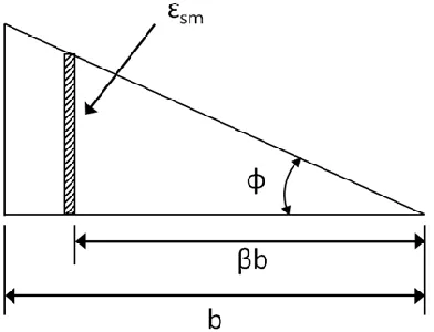
Where Goodsir assumed a strain distribution only between longitudinal reinforcement, Paulay and Priestley assumed the strain to be distributed as shown in Figure 11, where b is the thickness of the wall and b is the transverse distance between the wall’s edge and the extreme layer of reinforcing steel. Solving for the radius of curvature in terms of the residual strain in the longitudinal steel results in (1.6).

Figure 11 Strain profile for a cross section of buckled wall of thickness "b"

sm b R 



(33)

18

Solving (1.5) and (1.6) for the eccentricity ratio , given as   b, results in the final form (1.7), which can be used to calculate the eccentricity ratio imparted by a given residual strain. Conversely, it can be used to calculate the tensile strain associated with a wall’s maximum supported eccentricity ratio.

2

8 sm o

b

 



 

 _ _

  (1.7)

Where:

b

 = distance from the interior side of the wall to the extreme longitudinal reinforcement

sm



= residual strains in the extreme longitudinal steel

o = height of the buckled region

 = out-of-plane displacement of the wall

To develop an upper limit to the eccentricity ratio, Paulay and Priestley used force and moment equilibrium over an assumed compression zone as seen in Figure 12. This compression zone utilizes an equivalent stress block in both directions, where



is the compression zone’s depth of the in-plane direction and

a

is the compression zone’s depth in the out-of-plane direction.

Figure 12 Cross section of wall compression zone experiencing buckling

α

(34)

19

Considering the in-plane direction for a given length of the end region



and using the notation found in Figure 13, the concrete compressive force, C_c can be shown to be (1.8),

where



l is the longitudinal reinforcement ratio in the compression zone undergoing

buckling.

Figure 13 Internal forces for the buckling end region of a wall [46]

1 l y c

b f

C  

 



 



 

 

(35)

20

Solving for the ratio  in the out-of-plane direction and assuming an equivalent rectangular stress block results in (1.9).

' 1

1

2 0.85

c c

C

f b





 

 _  _

  (1.9)

Substituting (1.8) into (1.9) and rearranging to solve for the maximum eccentricity ratio,



_cr gives (1.10), where m is the mechanical reinforcement ratio for the end region. The right hand limit represents the wall failing if the out-of-plane displacement causes the load resisted by the section to extend outside the lateral boundaries of the wall. When this critical value is exceeded, the structural wall fails due to out-of-plane instability and buckles.



2



'

0.5 1 2.35 5.53 4.70 0.5 ; l y

cr

c

f

m m m m

f



       (1.10)

Paulay and Priestley calculated the expected longitudinal steel residual strains in the plastic hinge region to cause buckling for “Wall 2” tested by Goodsir [16]

and compared it to strains measured prior to buckling. The authors also used their buckling model to calculate ultimate displacement ductility for a series of masonry T-section walls previously tested by Priestley, Seible and Calvi[48]. In both instances, the predictions showed relatively close agreement with results from the experimental tests given the somewhat coarse assumptions made by the model.

(36)

21

making assumptions regarding axial load, geometry, and reinforcement detailing results in a simplified design expression for minimum thickness of the form (1.12). For singly reinforced walls, the thickness calculated, b increases by a factor of 1.26.

2 8 sm o b       _ _

  (1.11)

0.019 p

b 



 (1.12)

2.2.3 Lateral Stability of Reinforced Concrete Columns under Axial Reversed Cyclic Tension and Compression, Chai and Elayer [7]

Chai and Elayer performed a series of tests on reinforced concrete columns to simulate the end region of a structural wall and adjusted the model proposed by Paulay and Priestley to account for the new experimental data. Paulay and Priestley[46] previously derived the tensile strain,



_sm necessary to induce local lateral instability, repeated as (1.13). However, this method does not account for the hysteretic behavior for the reinforcing steel. In order to adjust for this, they proposed another form of



sm shown as (1.14).

2 8 sm o b   _ _ 

  (1.13)

* sm e r a

      (1.14)

Where: e

 = strain elastically recovered during initial reloading r

 = additional reloading strain required to yield the reinforcement in compression *

a

(37)

22

Both the elastic strain, _e and recovery strain,_rwere assumed to be proportional to the yield strain of the longitudinal steel, of the forms   _e  ₁ _y and   _r  ₂ _y. During experimental testing ₁ was found to range from 1 to 1.5 and ₂ was found to vary from 3 to 5. In order to calculate the residual tension strain *_a, Chai and Elayer[7] proposed (1.15), a modified version of Paulay and Priestley’s model.

2

* 2

a

o b

  _ _ 

  (1.15)

Where the previous model assumed a constant curvature throughout the plastic hinge region, Chai and Elayer[7] assumed a more realistic (but less conservative) sinusoidal curvature distribution. They also recommended slightly conservative values of ₁1 and

2 2

  , which results in lower values of strain being supportable prior to buckling. This simplifies the expression to (1.16), the final form for the maximum tensile strain _sm. For comparison, Paulay and Priestley’s[46]

formulation is provided again as (1.17).

2

2 ₃

sm y

o b

  _ _  

  (1.16)

2

8

sm

o b

  _ _ 

  (1.17)

(38)

23



2



'

0.5 1 2.35 5.53 4.70 0.5 ; l y

cr

c

f

m m m m

f



       (1.18)

Following Goodsir’s method of testing prisms[17], fourteen 4x8 inch rectangular column prisms were constructed and experimentally tested to help verify the accuracy of the new model. It was observed that the new modified strain equation (1.16) showed better agreement with the test results than Paulay and Priestley’s[46]

prior strain equation (1.17). However, both were conservative, underestimating the maximum tensile strain supportable prior to buckling upon a load reversal.

2.2.4 Minimum thickness of ductile RC structural walls, Chai and Kunnath[8]

Chai and Kunnath calculated minimum thicknesses for walls of varying heights, lengths, wall-to-floor ratios, and steel reinforcement ratios when subjected to ground motions. Acceleration demands with a peak ground acceleration of 0.4g were selected for analysis, corresponding to UBC seismic intensities designed for in "zone IV" seismic areas. Site effects such as soil variance and differences in attenuation across seismic frequencies were accounted for by varying peak ground acceleration to peak ground velocity ( / )a v

ratios. Required thicknesses were calculated using Chai and Elayer's[7] buckling strain formulation and Paulay and Priestley's[46] stability criterion, which were compared to thicknesses required by New Zealand Standards of 1995[36] (NZS) and the Uniform Building Code of 1996[51] (UBC).

(39)

24

walls tending to result in a longer period and acceleration spectrum demand. Similarly, smaller wall-to-floor area ratios resulted in a general increase in required wall thickness. Minimum wall thickness was insensitive to changes the tributary floor weight, and instead was overly affected by changes in wall height, with shorter walls resulting in larger required thicknesses. Lower levels of longitudinal reinforcement resulted in thinner required thicknesses, but the effect was less pronounced as low levels of reinforcement ratio.

Comparing the authors' calculated thicknesses to those required by NZS and UBC, the author's calculated required thickness agreed better with those determined by NZS in most cases. Taller, slender (large H_w t_w ratio), and more square (small H_w L_w ratio) walls showed poorer agreement between minimum thicknesses. Walls with above average ( / )a v

seismic ratios, large reinforcement ratios and large wall-to-floor ratios were also found to show poorer agreement among calculated thickness requirements. Paulay and Priestley suggest that prior to possible code revision, additional experimental research on plastic buckling be performed to assess the accuracy of the existing code requirements and buckling models.

2.3Design Code Considerations

(40)

25

limitations on aspect ratios, geometry, and reinforcement ratios, or design methods that indirectly result in limitations on such properties.

2.3.1 Uniform Building Code 1996 Vol. 2 [51]

The Uniform Building Code (UBC) of 1996 attempts to prevent lateral instability in walls resisting both axial and flexural loads by requiring a minimum wall thickness sixteen times the wall's clear (between floors) height, shown as (1.19). While this limitation is likely too simple to accurately design against plastic buckling, it does ensure some level of out-of-plane stiffness. Unfortunately, the limit does not scale with wall heights, resulting in an mistakenly constant minimum thickness as long as story height does not change.

16 cl w

H

t  (1.19)

(41)

26

2.3.2 American Concrete Institute Building Code Requirements (ACI 318-08)[1]

Wall detail requirements in ACI are similar to those in the UBC(1996)[51] in that lateral stability is considered for wall design, but plastic buckling is not directly addressed. Second order analyses based on applied loads, limits to out-of-plane service, minimum wall thicknesses, and specially reinforced boundary element requirements all are similar in function to those found in the UBC and do not provide a reliable and accurate method to prevent local plastic buckling.

Empirically designed walls have a unique design methodology with additional wall thickness requirements similar to the UBC's approach, and are shown as (1.20). It should be noted that these requirements generally result in a smaller thickness being required than those required by (1.19), and despite empirical walls limiting eccentric loading, plastic buckling does not require out-of-plane loads to occur.

100

25 25

u u

w w w

H L

t  and t  and t  mm (1.20)

(42)

27

boundary elements are not required by NCh to have additional transverse reinforcement and confinement and instead are simply required to resist applied overturning demands. This allowance was made following the good performance of buildings with poorly confined and unconfined end regions in the Viña del Mar 1985 earthquake. This change is expected to result in poorer performance of structural walls during seismic events where cyclic loads are likely to cause rapid spalling and a loss of poorly confined core concrete.

2.3.4 New Zealand Concrete Structures Standard (NZS 3101:1995,2006) [36][46]

The New Zealand Concrete Structures Standard currently provides guidelines that are meant to prevent plastic lateral instability in thin walls. NZS 3101:1995[36] requires for walls to meet the minimum required thickness, b_req as calculated using (1.21), (1.23) and (1.24). These equations are simplified approximations from Paulay and Priestley's[46] research and recommendations. NZS 3101:2006[37] changed the calculation of b_req to (1.22) , adding a factor _r to account for whether a wall is reinforced in a single layer or multiple layers and simplifying the calculation of _ to the factor  , which has predetermined constant values.



2



2



(NZS :1995)

1700 3101

m r w

req

k A L

b 



 

 (1.21)



2



(NZS : 2006)

1700 3101

r m r w

req

k A L

b  





 (1.22)



0.25 0.055



1.0

(43)

28 ' 0.3 0.1 2.5 l y c f f 

    (1.24)

Where: req

b = Required wall thickness

_ = Displacement ductility demand on the wall r

 = 1.0 for doubly reinforced walls and 1.25 for singly reinforced walls  = 5 for limited ductile plastic regions, 7 for ductile plastic regions

r

A = Aspect ratio (total wall height divided by wall length) w

L = Wall length

n

L = Wall clear height between floors

l

 = Longitudinal reinforcement ratio in the end region of the structural wall y

f = Steel yield stress '

c

f = Concrete compressive stress

When (1.22) controls the thickness of the wall at the end regions, NZS 3101:1995[36] provides additional requirements suggested in Paulay and Priestley's work [46], shown as (1.25) and utilizes dimensions depicted in Figure 14. These additional limits aim to prevent the design of boundary elements prone to lateral instability. Though NZS specifically imposes limits to prevent plastic buckling, the codified equations are heavily simplified expressions for generalized wall systems, possibly resulting in a loss of accuracy in cases where wall properties or seismic demands differ from those assumed.

2 1 1 10 w wb b

(44)

29

(45)

30

CHAPTER 3.EARTHQUAKES OF INTEREST

3.1Introduction

On September 4, 2010, a series of large seismic events began to occur around the area of Christchurch, NZ over a year's time. This section gives a general overview of the two most largest events: the Darfield and Christchurch earthquakes. The Darfield event was followed by several thousand smaller, successive aftershocks. Despite many seismologists considering the Christchurch event to be an aftershock of the Darfield earthquake, it will be discussed as a separate earthquake due to the earthquake's impact on the people and infrastructure of New Zealand. The general progression and magnitude of these events can be seen in Figure 15. Size and darkness of the circles corresponds to the relative magnitude of each event. Additional information regarding each event is provided in the following sections.

Figure 15 Magnitude of seismic events following the Darfield Earthquake (Data: Geonet[19])

Darfield Earthquake Sept. 4, 2010

Christchurch Earthquake February 22, 2011

Major Aftershock Sept. 8, 2010

Minor Aftershock Dec. 26, 2010

(46)

31

3.2Darfield Earthquake (September 4th, 2010)

The Darfield earthquake (also referred to as the Canterbury earthquake) occurred at 4:35 am (NZDT) on September 4, 2010 with a moment magnitude of 7.1 Mw. The epicenter

was located 10 km southeast of the city Darfield and was relatively shallow with a focus approximately 10 km deep[11]. Figure 16 contains accelerations measured during the event by seismographs stations in the surrounding area: red arrows display the maximum vertical acceleration while blue arrows indicate the maximum horizontal acceleration recorded, independent of their direction of travel. The relative size of the arrows corresponds to the magnitude of the acceleration. The largest peak ground accelerations near the area were 1.26 g vertically and 0.76 g horizontally. All stations surrounding the surface rupture had vertical-horizontal acceleration ratios greater than 1.5. These large vertical accelerations are thought to have exacerbated damage caused by the already large horizontal motions[11].

Figure 16 Ground accelerations from Darfield Earthquake [41]

Darfield Earthquake Epicenter

(47)

32

The soil in the area is largely variable, but typically consists of a mix of fine particles from glacial silts/clay particles and some volcanic rock. This soft soil resulted in a large amount of seismic attenuation before reaching Christchurch, with demands generally lessening as they approached the city center. The epicenter also occurred in largely rural area away from larger structures. For both of these reasons, the Darfield earthquake resulted in no deaths and only two injuries: one from a falling chimney and another from broken glass [11]. Damage was primarily limited to small residential properties (typically unreinforced masonry buildings) and occurred as a result of differential foundation settling caused by stress-induced lateral spreading and liquefaction. Areas subjected to liquefaction also experienced sand boils, where a fine soil particles and water were forced to the surface, leaving behind deposits[18] as seen in Figure 17.

(48)

33

Examining damage occurring beyond that caused by geotechnical issues, damage was concentrated in the many unreinforced masonry (URM) buildings within the Darfield region. A follow-up investigation surveyed 595 of the 958 URM structures in the area and found 125 to be unsafe for continued use, and 167 required repairs before continued use. Some URM buildings that had undergone partial or full seismic retrofitting withstood the earthquake with only minor damage. Those without retrofits fared poorly due to having limited deformation capacities. Buildings also experienced non-structural damage such as broken windows, minor damage to cosmetic elements, and varying levels of damage to building components and contents [11].

3.3Darfield Aftershocks

In the weeks following the Darfield earthquake, thousands of aftershocks were reported to have Richter magnitudes of ML > 2 and eleven larger aftershocks of ML > 5.0

occurred around the fault line. Again, these events were characterized by large vertical-horizontal acceleration ratios. A major ML 5.2 aftershock struck September 8, 2010. This

(49)

34

Figure 18 Darfield Earthquake and Subsequent Aftershocks [16]

Damage from the Darfield aftershocks was typically less serious in magnitude, but of a similar nature to that of the primary earthquake: damage due to foundation spreading and liquefaction and a concentration of damage in unreinforced masonry buildings. Despite these aftershocks, many businesses reopened within two weeks of the initial event. Buildings too damaged to be repaired and deemed unsafe and unstable were demolished in the following weeks and months [11].

Darfield Earthquake, September 4th

(50)

35

3.4Christchurch Earthquake

The Christchurch earthquake (also referred to as the Lyttelton aftershock) occurred at 12:51 pm (NZDT) on February 22, 2011 as a continuation of the seismic events following the Darfield earthquake. The epicenter of the moment magnitude 6.3 Mw earthquake was located

8km southeast of Christchurch, the largest city-center on the South Island. The event was relatively shallow with a focus approximately 4km deep.[15]

Figure 19 Ground accelerations from Christchurch Earthquake [41]

Figure 19 contains accelerations measured during the event: red arrows display the maximum vertical acceleration while blue arrows indicate the maximum horizontal

Christchurch Building District

(51)

36

acceleration recorded, independent of their direction of travel [41]. Again, recorded vertical accelerations were larger than expected, often exceeding the horizontal accelerations by a factor of 2. When compared to the same depiction of the Darfield event in Figure 16 it can be seen that due to the close proximity of the epicenter, peak ground accelerations within Christchurch are much larger, often exceeding 1g inside the Christchurch Building District (CBD) and nearing 2g’s in the surrounding areas.

Again, the soil in the area was comprised of fine particles from glacial silts and clay particles and volcanic rock. Despite the soft soil, the proximity of the event to the CBD led to 185 deaths and a large number of injuries as a result of liquefaction, rock falls and structural damage leading to the collapse of many buildings. Liquefaction was much more pronounced during this event, affecting as much as 50% of Christchurch and the surrounding areas [15]. Figure 20 demonstrates the severity of the liquefaction and differential settling, while Figure 21 shows two rock falls near Redcliffs, a town East of Christchurch.

(52)

37

Figure 20 Examples of liquefaction (Left) and differential settling (Right) [15]

Figure 21 Two different rock falls near Redcliffs, east of Christchurch [15][11]

Figure 22 Post-earthquake collapse of the Canterbury Television building (Left[20]) and Pyne Gould

(53)

38

Figure 23 Damage incurred by the Pacific Brands House (Courtesy of Sri Sritharan)

(54)

39

model and Chai and Elayer's buckling model to help assess the models' accuracy. These structures, the damage they incurred, the non-linear analyses performed, and their respective results are discussed in CHAPTER 7.

It should be noted that additional buildings (most notably the Smith City Parking Deck, among others) also experienced excessive damage or collapses. These structures are not discussed here due to having no structural walls or because their walls were formed a “closed” shear core that lacked significant instability to be considered within the scope of this thesis. Beyond these specific buildings, hundreds of unreinforced masonry (URM) structures collapsed or experienced heavy damage. These collapses caused relatively few deaths or injuries due to local authorities closing or limiting access to many of these buildings after initial damage from the Darfield event. URM buildings retrofitted to more current standards prior to the Christchurch event generally sustained less damage than those left un-renovated. Steel structures fared particularly well, with only a few structures being red-tagged as unusable[11].

3.5Christchurch Aftershocks

(55)

40

CHAPTER 4. RESEARCH METHODS

4.1General Discussion

As previously mentioned, this project utilized a range of methods and tools to calculate displacements and strains within walls subjected to various axial and horizontal loadings. A modified version of Cumbia[30] was used to estimate force-displacement responses of individual members for comparison with prior experimental results and to conduct a parametric study on the selected buckling models. The three buildings selected as part of a case study were modeled in the analysis program SAP2000v14[13] and were subjected to non-linear time history analyses. Specifics regarding the program Cumbia and its modification for use with wall systems are given below. Due to the range of information conveyed, each of the three analyses performed in SAP2000v14 are discussed at length in Section 7.2.

4.2Cumbia

(56)

41

capacities, as suggested by Priestley, Calvi and Kowalsky[47]. Cumbia was originally intended for the sectional analysis of rectangular or circular members rather than walls, leading to a modifications being made to account for this difference. The modified program is referred to as CumbiaWall to prevent confusion between the original program and the adjustments made for analyses performed in this thesis. Additional information regarding the operation of Cumbia and the methods it uses to calculate values for displacement, strains, and forces can be found in the user manual[31]. Code for the modified version of CumbiaWall and an example of its input is provided in Appendix A. The program was neither created nor tested for general use, and great care should be taken in verifying any output provided.

4.2.1 Variance of Confinement

Cumbia calculates an average level of confinement for an entire cross-section. While this approximation negligibly affects results for smaller, more regular cross-sections, it may lead to inaccurate results when analyzing structural walls. This is because walls often have additional reinforcement in their end regions and significantly less confined web regions. To adjust for this, CumbiaWall divides the cross-section into sub-sections where confinement is calculated individually. Figure 24 shows two examples of the sub-division's implementation.

(57)

42

simplify connecting sub-sections' geometries and was found to have negligible effect on results for the cases considered.

Figure 24 Example of sub-dividing a rectangular wall (Left) and a barbell wall (Right) for analysis

It is important to note that this approach can result in high levels of concrete strength in end regions and low levels of concrete strength in webs. While it is likely some interaction between end region confining steel and the web leads to a gradual transition between end region concrete strength and web concrete strength, CumbiaWall models the transition as a discrete change at the end region and web interface. Though such an instantaneous drop in strength is unlikely, crushing of web concrete occurs in walls with thicker boundary elements

Confined Region1

Confined Region 2

Confined Region 3 Unconfined Region 1

Unconfined Region 2

(58)

43

and sparse web confinement and is typically concentrated at the ends of the web. This suggests the concrete strength "transition zone" between levels of confinement is relatively short in length, and therefore its effect was assumed to be negligible.

4.2.2 Calculation of Longitudinal Steel Reinforcement Ratio

CumbiaWall was also utilized to calculate the displacement at which the selected buckling models predict failure. As previously discussed, both models’ stability criterion is based upon the mechanical reinforcement ratio, '

/ l y c

(59)

44 4.2.3 Calculation of Plastic Hinge Lengths

While Cumbia calculates plastic hinge lengths for a member in single bending following the recommendations from Priestley, Seible and Calvi[48] of the form (1.26), CumbiaWall uses a conservative modification (1.27) as suggested by Priestley, Calvi and Kowalsky[47] based upon previous work by Paulay and Priestley[45]. The new method utilizes the effective height of the wall instead of the contraflexure length. The additional term 0.1Lw is introduced to adjust for additional strain penetration induced by the larger amounts of tension shift commonly found in wall systems. Similarly, (1.28) is a modification suggested for masonry walls by Priestley, Calvi and Kowalsky[47], which takes into account the typical reduced bond capacity and increased strain penetration seen in prior experimental work.

2

P c sp sp

L   k L L  L (1.26)

0.1 2

P e w sp sp

L  k H  L L  L (1.27)

0.04 0.1 3

P e w sp sp

L  H  L L  L (1.28)

Where:

k = 0.2 u 1 0.08

y f f           c

L = distance to point of contraflexure, typically L for members in single bending e

H = wall effective height, taken as 2

3 Hw    

  , the height of the wall sp

L = 0.022f d_y _bl u

f = ultimate strength of local longitudinal reinforcement y

f = yield strength of local longitudinal reinforcement bl

(60)

45 4.2.4 Shear Strength

Cumbia[30] also calculates the shear strength envelope using the revised UCSD shear model[25]. The structural walls examined in this thesis are generally tall and slender, with a response dominated by flexural action. Due to this, CumbiaWall assumes shear strength to be a non-issue. CumbiaWall calculates shear deformations using the same method as Cumbia following the procedure outlined by Montejo[31] and initially provided by Priestley, Calvi and Kowalsky[47] as outlined below.

5 6

s g

A  A (1.29)

' ' y eff c y M I E

 (1.30)

eff s sg

I A k

L

 (1.31)

,

eff s eff sg

g I

k k

I

 (1.32)

2 , 0.25 0.6 0.25 10 y

s cr s

y y

k  E D

 



 (1.33)

(61)

46

(62)

47

CHAPTER 5. EXAMINATION OF PRIOR EXPERIMENTAL RESULTS

5.1Introduction

Many past researchers have performed experimental tests on structural wall systems and their boundary elements while focusing on other topics such as the effects of seismic detailing, ductility, and nearly countless other topics. Where out-of-plane failures occur during these tests, many authors attribute the failure to a general lateral instability, but few distinguish between a global, elastic failure of an entire specimen and the local, plastic failure of a wall’s end region. Aside from the prior works reviewed, little to no research examines the failure mechanism of plastic out-of-plane buckling in great depth. Additionally, the prior models have been compared with a small selection of experimental wall test results, providing a limited understanding of the models’ accuracy. To address this, this section reviews a large number of prior experimental tests and compares their results with those predicted by models proposed by Paulay and Priestley [46] and Chai and Elayer[7].

(63)

48

comparison of each specimen’s results with those predicted by the selected buckling models. In all, sixty-three tests on structural walls and forty-three tests on boundary prism elements are examined. Appendix C contains tables of information for each wall and prism specimen considered: Table 16 through Table 18 contains loading, dimensions, material properties and reinforcement details for wall specimens. The same information for prism specimens is provided in Table 20 through Table 22.

5.2Experimental Tests of Structural Walls

5.2.1 Goodsir [17]

(64)

49

(65)

50

(66)

51

Due to the slenderness of the walls, all four specimens experienced lateral instability in their end regions and buckled locally. The T-section experienced lateral instability only in its web, but continued to sustain loads in the reverse direction until the flange failed in compression under successively larger compressive cycles. Figure 27 displays the typical buckling failure mode. The buckled end region is circled, and the displaced shape’s centerline is traced with a dashed line.

Figure 27 Typical local buckling damage seen in Goodsir’s walls [17]

5.2.2 He and Priestley [48]

(67)

52

scaled dynamic loadings. In both cases an additional compressive axial load was applied. Walls were subjected to a pair of load reversals to a pre-determined ductility level, followed by a load cycle to half-yield and another cycle to quarter-yield. If a wall continued to sustain load, the process was repeated by incrementing the loading of the first two cycles to induce a higher level of ductility. The half-yield and quarter-yield cycles remained constant in magnitude throughout the test, only the "ductile" cycles were incremented. All walls had uniform amounts of longitudinal steel along their web and flange, which was placed in a single layer at the center of the masonry blocks and grouted in place. Horizontal reinforcing steel consisting of a single rebar per layer was typically spaced closer together in the web than the flange. Figure 28 shows the typical reinforcing pattern for these T-walls.

(68)

53

In a majority of the nine tests, the walls failed with their web in compression. It is important to note again that the specimens only have a single layer of reinforcement and are significantly less stable laterally. Prior to failure, there was little indication of an impending failure beyond small out-of-plane deflections. As a result, it is difficult to determine if walls failed due to local instability or due to bar buckling. Inspection of images preceding collapse led to assuming that four walls buckled due to lateral instability. The walls that buck