Clock Synchronization in Wireless Sensor Networks: Performance Analysis and Protocol Design.

(1)

ABSTRACT

GONG, FENGYUAN. Clock Synchronization in Wireless Sensor Networks: Performance Analysis and Protocol Design. (Under the direction of Dr. Mihail L. Sichitiu.)

Time synchronization is a fundamental problem in any distributed system. In particular, wireless sensor networks (WSNs) require scalable, energy efficient time synchronization for implementing dis-tributed tasks on multiple sensor nodes. We propose an energy efficient Coefficient Exchange Synchro-nization Protocol (CESP) based on a receiver-receiver synchroSynchro-nization scheme, which minimizes the impact of access-time delays. Most of the existing synchronization protocols focus on improving the synchronization accuracy by assuming the availability of MAC-level timestamping with little concern for power consumption. The proposed time synchronization protocol achieves high synchronization ac-curacy similar to the classic Reference Broadcast Synchronization (RBS) protocol without requiring packet-level timestamping but with a significant reduction on communication overhead to achieve low power consumption.

Different synchronization schemes and hardware systems are able to achieve widely different lev-els of synchronization accuracy. Since synchronization accuracy is very sensitive to random delays and clock rate fluctuations, we evaluate the pairwise synchronization error as a function of random delays and clock drifts, to quantitatively evaluate synchronization performance as a function of the relevant parameters, such as the beacon interval, the number of beacons per synchronization period, and the measurement point. The synchronization error is analyzed for different state-of-the-art pairwise syn-chronization schemes, based on one-way sender-receiver, two-way sender-receiver and receiver-receiver approaches, using application layer or medium access control (MAC) layer timestamping. The models are validated through numerical and experimental results.

(2)

Clock Synchronization in Wireless Sensor Networks: Performance Analysis and Protocol Design

by Fengyuan Gong

A dissertation submitted to the Graduate Faculty of North Carolina State University

in partial fulfillment of the requirements for the Degree of

Doctor of Philosophy

Computer Engineering

Raleigh, North Carolina

2016

APPROVED BY:

Dr. Harilaos Perros Dr. Mihail Devetsikiotis

Dr. Rudra Dutta Dr. Mihail L. Sichitiu

(3)

DEDICATION

(4)

BIOGRAPHY

(5)

ACKNOWLEDGEMENTS

I would first like to thank my advisor Dr. Mihail L. Sichitiu for his tremendous help during my entire course of Ph.D. study. Dr. Sichitiu not only guides me conducting research using scientific method and thinking, but also leads me to be self-motivated and self-learning. Dr. Sichitiu is more like a friend than an advisor, sharing his thoughts on research, careers, life, and everything.

I would also like to thank my advisory committees, Dr. Harilaos Perros, Dr. Mihail Devetsikiotis, and Dr. Rudra Dutta for their continuous support and advising.

I would also like to acknowledge Dr. Alexandra Duel-Hallen, Dr. Gregory T. Byrd, Marhn Fullmer, lab-mates, and all my friends who supported and helped me.

(6)

LIST OF TABLES

(9)

LIST OF FIGURES

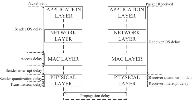
Figure 1.1 Delay stack model between transmitter and receiver. . . 2

Figure 3.1 Pairwise synchronization topologies where a slave node(s) wants to obtain an estimate of a master node’s time: (a) sender-receiver based synchronization, where the slave node directly synchronizes with the master node; (b) receiver-receiver based synchro-nization, where the slave node synchronizes with the master node with the help of a common reference node. . . 18 Figure 3.2 One-way sender-receiver synchronization timing diagram during the transmission and

reception of thekth synchronization packet, where thetM aster andtSlave denote the

time scales at the master and slave nodes, respectively. . . 19 Figure 3.3 Two-way sender-receiver synchronization timing diagram during the transmission and

reception of thekth synchronization packet and reply. . . 19 Figure 3.4 Receiver-receiver synchronization timing diagram during the transmission and

recep-tion of the kth synchronization packet. . . 20

Figure 4.1 Example of a multihop network topology using CESP and RBS: (a) the physical graph specifying physical connectivity; (b) CESP synchronization logical graph with dash line drawn between nodes that can receive from a common reference node (marked in

<> on each edge), and therefore can synchronize their clocks to each other; (c) RBS synchronization logical graph if RBS does not enable reference node to forward local timestamps of master node; (d) CESP synchronization spanning tree corresponding to (b) with node 1 as the root; (e) RBS synchronization spanning tree corresponding to (c) with node 1 as the root. . . 29 Figure 4.2 Probability distribution function of sender-side uncertainty with mean of 6.31msand

standard deviation of 3.05ms. . . 31 Figure 4.3 Comparison of the average synchronization errors performance while changing the

number of broadcast beacons used by the algorithm when the beacon interval is fixed at ∆Tb = 1s in a 6 h trace and the moving average coefficients of CESP-MA are set

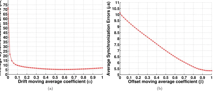
to α= 0.55 andβ= 1, with and without MAC-layer timestamping. . . 32 Figure 4.4 Synchronization error performance of CESP-MA whenk= 12 and ∆Tb= 10swith a

minimum synchronization error of 5.33µs, which improves error performance by 15.8% and 24.2% compared with RBS and CESP (mean(RBS) = 6.33µs;mean(CESP) = 7.03µs) while: (a) changing the drift moving average coefficientαwhen fixingβ at 1, and; (b) changing the offset moving average coefficientβ when fixingαat 0.55. . . 33 Figure 4.5 CESP synchronization accuracy performance averaging over 1000 Monte Carlo rounds

by simulating different packet error rate using the experimental trace without MAC-layer timestamping whenk= 5, ∆Tb= 1s,α= 0.55, andβ = 1. . . 33

Figure 4.6 Physical graph of the triangle topology where node 1 is the root node. . . 34 Figure 4.7 Synchronization logical graph of triangle topology with dash-dot line drawn between

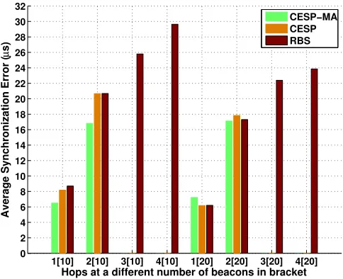
nodes that have received from a common reference node (marked in<> beside each edge) for (a) CESP and CESP-MA, and (b) RBS. . . 35 Figure 4.8 Multihop synchronization error performance of triangle topology at a different number

of broadcast beacons used by the algorithm when fixing the beacon interval at ∆Tb=

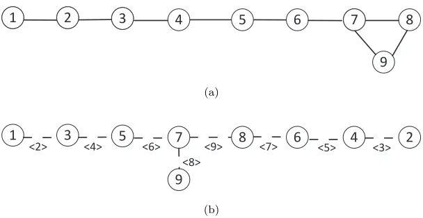
10susing RBS, CESP and CESP-MA in a 6 h trace. . . 35 Figure 4.9 Multihop chain topology: (a) physical graph where node 1 is the root node; (b)

(10)

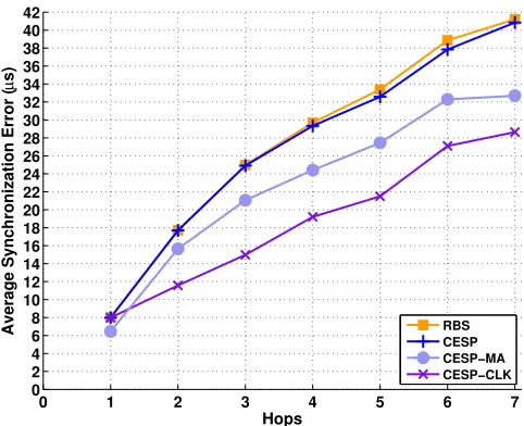
Figure 4.10 Multihop synchronization error performance of chain topology as a function of the number of synchronization hops from the reference node at the number of broadcast beacons used in the algorithm k = 10 when fixing the synchronization period at

Ts= 2.5 minutes using RBS, CESP, CESP-MA and CESP-CLK in a 6 h trace. . . 37

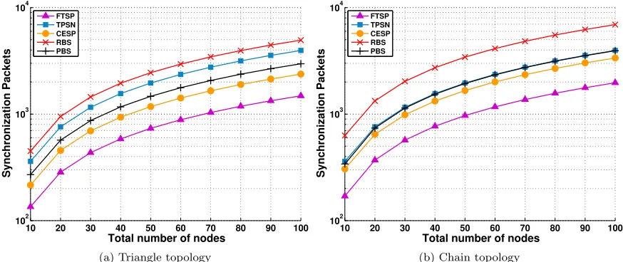
Figure 4.11 CESP power savings over state-of-the-art protocols in multiple topology as a function of the number of beacons used by the algorithm. . . 40 Figure 4.12 Number of synchronization packets sent and received in the triangle and chain topologies. 41

Figure 5.1 Pairwise synchronization error analysis diagram, where ED represents the effective delay defined in Definition 1, and the dot line denotes the source of the effective delay by either MAC-layer or APP-layer timestamping, whereas the dash line only applies when using APP-layer timestamping. . . 43 Figure 5.2 Comparison of numerical synchronization error and theoretical results for one-way

sender-receiver schemes while varying (a) ∆Tb; (b)k; (c) ∆t. . . 56

Figure 5.3 Comparison of numerical synchronization error and theoretical results for two-way sender-receiver schemes while varying (a) ∆Tb; (b)k; (c) ∆t. . . 57

Figure 5.4 Comparison of numerical synchronization error and theoretical results for receiver-receiver schemes while varying (a) ∆Tb; (b)k; (c) ∆t. . . 57

Figure 5.5 PDF of: (a) OS delay with a mean of 1.291msand a standard deviation of 9.344µs; (b) OS and access delays with a mean of 6.31msand a standard deviation of 3.05ms. 59 Figure 5.6 Comparison of experimental synchronization error and theoretical results for one-way

sender-receiver schemes while varying (a) ∆Tb; (b)k; (c) ∆t. . . 60

Figure 5.7 Comparison of experimental synchronization error and theoretical results for two-way sender-receiver schemes while varying (a) ∆Tb; (b)k; (c) ∆t. . . 61

Figure 5.8 Comparison of experimental synchronization error and theoretical results for receiver-receiver schemes while varying (a) ∆Tb; (b)k; (c) ∆t. . . 61

Figure 6.1 Simulation topologies of (a) pairwise where slave node 2 synchronizes with master (reference) node 1; (b) two-hops where nodes 2 and 3 synchronize with the reference node 1, and slave node 4 synchronizes with master nodes 2 and 3; (c) grid network with 100 nodes where corner nodes 1, 10, 91, and 100 are reference nodes and each node only connects with its horizontal and vertical neighbours. . . 70 Figure 6.2 Comparison of the pairwise synchronization offset and skew performance in constant

temperature environment while changing the STD of measurement noise when fixing the skew noise STD in a 10 minutes trace. . . 72 Figure 6.3 Time series of the real skew and the accumulated offset in comparison with the

es-timated skew and offset using FTSP, TSVP, Kalman-Temp, and Kalman-CONST in constant temperature environment when the measurement noise and skew noise STDs are 10ms and 5ppm, respectively. . . 73 Figure 6.4 Comparison of the pairwise synchronization offset and skew performance in constant

temperature environment while changing the STD of skew noise when fixing the mea-surement noise STD in a 10 minutes trace. . . 74 Figure 6.5 Variable temperature trace used in the simulations. . . 74 Figure 6.6 Comparison of the pairwise synchronization offset and skew performance in a

temper-ature varying environment while changing the STD of measurement noise when fixing the skew noise STD in a 10 minutes trace. . . 75 Figure 6.7 Comparison of the pairwise synchronization offset and skew performance in a

(11)

Figure 6.8 Comparison of the multihop synchronization offset and skew performance of node 4 in Fig. 6.1(b) while changing the STD of measurement noise when fixing the skew noise STD in a 10 minutes trace, where nodes 3 and 4 are at constant temperature and node 2 is at variable temperature. . . 77 Figure 6.9 Comparison of the multihop synchronization offset and skew performance of node 4 in

Fig. 6.1(b) while changing the STD of skew noise when fixing the measurement noise STD in a 10 minutes trace. . . 78 Figure 6.10 Comparison of the large scale (shown in Fig. 6.1(c)) network-wide multihop

(12)

Chapter 1

Introduction

In this chapter, Section 1.1 presents the overview of wireless sensor networks (WSNs) and clock synchro-nization. Sections 1.2 and 1.3 present the motivation and contributions of this thesis, respectively. The outline of this thesis is shown in Section 1.4.

1.1 Overview

1.1.1 Wireless Sensor Networks

Recent developments in microelectromechanical systems (MEMS) and signal processing enable inte-gration of distributed sensing, computing, and communications into low-cost, low-power devices called wireless sensor nodes. These sensor nodes cooperate to forward packets through multihop communication and form WSNs. The increasing interest in WSNs leads to a variety of possible promising applications: home appliance control, military surveillance, environmental and human health monitoring [1]. In most applications, WSNs have limited energy resources, unreliable sensor nodes, and are often large scale.

1.1.2 Clock Synchronization

(13)

(MAC) [2]. Since sensor networks are expected to work for extended periods of time once deployed, it is common to set sensor nodes in sleep mode periodically to conserve the limited battery energy. Maintain-ing a relative time reference is essential for wakMaintain-ing up sensor nodes at coordinated times such that data exchange can be successful. It is thus highly desirable to use a simple and efficient clock synchronization mechanism where all timestamps refer to a single reference clock instead of multiple local clocks. Perhaps the two most important (and conflicting) requirements for such a synchronization protocol are high syn-chronization accuracy, and low power consumption. In many applications, a maximum synsyn-chronization error has to be maintained, which dictates the need for resynchronization, which in turn determines the power consumption.

Exchanging timing messages between nodes is commonly used for network time synchronization. When a node timestamps a synchronization packet for transmission at the application (APP) layer, multiple delays are encountered until the packet is successfully received and decoded at the intended receiver(s). These delays leading to inaccuracy in synchronization, can be classified into six main cate-gories [2] as shown in Fig. 1.1:

APPLICATION

LAYER

APPLICATION

LAYER

NETWORK

LAYER

NETWORK

LAYER

MAC LAYER

PHYSICAL

LAYER

PHYSICAL

LAYER

Sender OS delay

Receiver OS delay

Packet Sent _{Packet Received}

Access delay

Sender interrupt delay

Receiver interrupt delay

Sender quantization delay Receiver quantization delay

Transmission delay

Propagation delay

(14)

• OS delay: represents the delay from the APP-layer request down to the MAC-layer at the

trans-mitter (or MAC-layer up to APP-layer at the receiver), and it is highly dependent on the operating system (OS) scheduling and potential queues in the network and MAC layers;

• Access delay: due to the broadcast nature of wireless medium sharing, the packet has to wait until

the node can access the channel. In WSNs, this delay usually contributes greatly to the variability of packet delay in WSNs, and varies significantly with the MAC protocol used by the nodes and medium utilization;

• Interrupt delay: includes the delay from OS interrupts due to CPU multitasking, and it is highly

platform dependent with random variations;

• Quantization delay: models the delay due to round-off errors introduced by the digital system, and

it is dependent on the accuracy of system clock ticks;

• Transmission delay: includes the delay of transmitting the packet bit-by-bit by the transmitter,

and it is proportional to the packet’s length and inversely proportional to the transmission data rate;

• Propagation delay: models the delay necessary for the signal to travel from the transmitter to the

receiver, and it is proportional to the link length, and inversely proportional to the propagation speed.

(15)

1.2 Motivation

In WSNs without MAC-layer timestaming, the access delays usually dominate overall synchronization accuracy. Other factors resulting in inaccuracy of synchronization performance such as quantization delays, interrupt delays, and stability of the crystal oscillators are usually a much smaller source of inaccuracy than the access delays. Synchronization methods based on timing packet exchanges between a sender and a receiver are vulnerable to sender OS and access time uncertainties unless MAC-layer timestamping is used [4, 5]. Many recent time synchronization protocols [6–12] assume that MAC-layer timestamping is supported by the radio hardware while neglecting the fact that packet-level timestamping is not provided by all radio chipsets. To provide MAC-layer timestamping for transmitted packets, the radio chipset has to accept the bytes of the packet one after the other and signal the OS in some way that the current transmission is under way. Then, the OS has to modify the bytes of the packet currently being transmitted on the fly. Some system-on-a-chip devices [13–15] do integrate MAC timers and packet-level interrupts to support MAC-layer timestamping, but many modern radio modules for Zigbee [16], WiFi [17], and Bluetooth [18] are abstracting communication primitives at the packet level (i.e., the OS has to provide the packet to be sent with no further chance of modifying it). Thus, MAC-layer timestamping may not be available in many of the WSNs of the future. Furthermore, MAC-MAC-layer timestamping is of little use outside accurate time synchronization; hence, there is very little incentive on the chip manufacturers to provide support for it.

To remove sender-dependent randomness, when MAC-layer timestamping is not available, receiver-receiver synchronization schemes exchange received timestamped packets between receiver-receivers to achieve better synchronization accuracy at the expense of additional communication overhead [19]. Thus, it is important to design a synchronization protocol to reduce communication overhead without reducing the synchronization precision.

In addition to random delays, clock rate fluctuations result in clock drift between a pair of nodes over a period of time. To compensate for clock drift, linear regression has been employed on many time synchronization protocols [3, 4, 7, 9, 12, 19–29] to establish a linear model between clocks at different sensor nodes for long-term synchronization with low communication overhead. Thus, it is important to analyze the impact of random delays and clock rate fluctuations on pairwise synchronization using linear regression.

(16)

drift and offset, it performs poorly when environment factors affect the clock frequency often [30]. Accurate clock drift estimation is the key for providing long-term synchronization since the clock offset is accumulated through clock drifting; therefore, it is important to accurately model the clock drift according to its physical characteristics. Among the many environmental factors that affect the clock drift (e.g., temperature, humidity, source voltage), temperature is the dominant factor that significantly affects the clock drift’s performance. To compensate for the influence of temperature change on the clock drift, researchers proposed offline calibration methods to estimate the real clock drifts at various temperatures such that compensation is achieved during deployment based on the calibration table [31]. Instead of using offline calibration, recently, some researchers proposed to apply the Kalman filter to dynamically compensate for the clock drift online while assuming a constant clock drift model [32, 33]. However, the environment temperature may vary in most applications. Thus, it is important to model the clock drift as a function of the measured environmental temperature, while employing the Kalman filter to accurately track the drift changes taking into account the physical characteristics of the clocks. To extend pairwise synchronization to network-wide synchronisation, spanning tree based solutions are prone to propagate synchronization errors rapidly throughout the network such that leaf nodes may not be well synchronized with the root node [6]. Thus, it is important to design a protocol to reduce error propagation while utilizing multiple neighbours’ information asynchronously in a fully-distributed approach.

1.3 Contribution

The main contributions of this thesis are summarized as follows.

(17)

ac-curacy. CESP mainly focuses on pairwise synchronization with an extension to the multihop network synchronization based on the spanning tree and adaptive clock speed adjustment discussed in [12,19,34]. The performance of CESP is compared with the original receiver-receiver synchronization protocol, i.e., reference broadcast synchronization (RBS) [19], and other well-known time synchronization protocols.

Second, we model the relative synchronization error as a function of random delays and clock rate fluc-tuations in Chapter 5. The model can be used to predict the resulting performance of a synchronization scheme in a given system, and even to further design the parameters of the system (e.g., resynchroniza-tion period, number of probes, etc) required to achieve a desired accuracy. To quantitatively analyze the impact of random delays and clock rate fluctuations on synchronization accuracy, we focus on the er-ror performance in one-way sender-receiver, two-way sender-receiver and receiver-receiver schemes with APP-layer or MAC-layer timestamping while employing linear regression by changing three key parame-ters: the beacon interval, the number of beacons per synchronization period, and the measurement point (i.e., when is the synchronization accuracy checked relative to the synchronization period).

Third, we model the clock drift as a function of environmental temperature according to its physical characteristics, and to apply the Kalman filter to dynamically compensate for changes in the nodes’ clock drifts and offsets instead of using offline calibration in Chapter 6. We further extend pairwise synchronization into a temperature-compensated Kalman based distributed synchronization protocol namedTKDS, where each node utilizes multiple neighbours information asynchronously to reduce error propagation through the multi-hop network.

Although particularly useful in WSNs, the protocols (and models) presented in this thesis can also be used to synchronize nodes (and to evaluate the performance of time synchronization) on any com-munication network that allows the reception of broadcast packets on a bidirectional data transmission link.

1.4 Outline

(18)

(19)

Chapter 2

Related Work

Clock synchronization has been extensively studied in the past decades. Nodes equipped with Global Positioning System (GPS) can be easily synchronized in outdoor environments [35], but this may not be a desirable solution when considering the size, cost, power consumption, and availability of GPS reception. The most well-known and widely adopted online synchronization protocol in the Internet is Network Time Protocol (NTP) devised by Mills [36], where clients synchronize their local clocks to time servers through analysis of the round trip delay. However, using NTP leads to relatively low accuracy in synchronizing large-scale WSNs due to the non-deterministic access delays when accessing the medium, and to a large amount of communication overhead from maintaining the NTP connections. The recent high-precision synchronization standard IEEE 1588 [37] has improved synchronization accuracy up to sub-microsecond precision in the Internet by processing messages at lower physical layers, but requires frequent resynchronization and a large amount of communication overhead.

Since traditional clock synchronization schemes used in the wired network are not suitable for WSNs, Elson et al. [38] originally proposed a low-power, post-facto synchronization scheme implemented by RITS [25]. Recently, many high-accuracy and low-power synchronization protocols have been proposed; these approaches can be roughly categorized in the following three fundamental schemes based on how pairwise synchronization is performed.

One-way sender-receiver (1-way S-R)schemes synchronize multiple receivers with a single sender that

(20)

MAC-layer timestamping to achieve high precision. Recently, Lenzen et al. [6] showed that the global error of FTSP increases exponentially with the size of network, and proposed a scalable PulseSync protocol that overcomes the scalability drawback by rapid information flood. However, Yildirim et al. [7] pointed out possible drawbacks of rapid flooding and proposed a slope estimation strategy with minimum variance for linear regression [21], whereas Ferrari et al. [8] utilized interference during flooding constructively to propose a new flooding architecture.

Two-way sender-receiver (2-way S-R) schemes involve interactive pairwise communication between

a sender and a receiver [5, 10, 11, 24, 28, 35, 39–42]. Ganeriwal et al. [5] originally proposed the timing-sync protocol for sensor networks (TPSN) by using MAC-layer timestamping to remove the access delay uncertainties, but requiring relatively frequent resynchronization to achieve high precision due to the lack of clock drift compensation. To compensate for clock drift, TSVP [28] employs linear regression on TPSN, and maximum likelihood estimators are applied for jointly drift and offset estimations [43, 44].

Receiver-receiver (R-R)schemes achieve pairwise synchronization between pairs of receiving nodes

af-ter receiving beacons broadcasted from a common reference node [3,19,20,23]. Elson et al. [19] originally proposed the reference broadcast synchronization (RBS) to eliminate the sender-side delay nondeter-minism by exchanging all the received beacons’ timestamps between pairwise receivers, achieving a high pairwise accuracy of around 10 µs even without MAC-layer timestamping. Currently, no other time-synchronization protocol comes close to this precision without MAC-layer timestamping. To minimize power consumption, PBS [20] in receiver-receiver schemes overhears beacon exchange without sending extra synchronization packets. Recently proposed, CESP [3, 23] achieves a similar accuracy as RBS, but at a reduced communication overhead by exchanging synchronization coefficients.

(21)

clock distribution network from the multihop routing tree to have nodes choosing their synchronization neighbours that offer the greatest frequency stability. To derive the shortest-path spanning tree that achieves the optimal global synchronization, Karp et al. [34] used a maximum likelihood formulation on RBS [19] by modelling a minimum variance estimate based on global information.

A challenge in tree-based multihop synchronization is that the directly connected neighbouring nodes may not synchronize well if they are on different paths of the spanning tree [11]. Requiring no refer-ence node or tree construction, many fully-distributed synchronization protocols have been proposed by averaging out the local information only, mainly formulated as the consensus-based [10, 46–48] or gradient-based [11, 49–52] approaches assuming that the communication delay is negligible. To analyze the impact of random delays in consensus-based approaches, He et al. [53] proposed the weighted maxi-mum time synchronization (WMTS) and showed that only the clock skew (i.e., the derivative of offset) can be synchronized within acceptable accuracy. Recently, Leng et al. [54] proposed a distributed syn-chronization algorithm based on belief propagation by estimating only the clock offsets, achieving a better synchronization accuracy than consensus-based algorithms under Gaussian random delays, which is further extended to a joint estimation of both drift and offset in [55]. Ahmad et al. [56] derived a message-passing method for the clock offsets tracking in the presence of exponential random delays. However, none of the above synchronization algorithms considers the clock rate fluctuations with tem-perature changes.

In reality, the common assumption that the clock drift remains constant over a certain period of time is not valid in applications with frequent temperature fluctuations. To compensate for clock drift affected by temperature changes, Schmid et al. [30] first designed a software compensated crystal oscillator (SCXO) using measurements of the differential drift, and then proposed a temperature compensated time synchronization (TCTS) exploiting the on-board temperature sensors to prolong the resynchronization period in dynamic environments [57]. Yang et al. [31] proposed to directly remove the clock skew during the external synchronization and then to dynamically compensate the effect of the clock skew according to the working temperature. Recently proposed, TACO [58] estimates the correlation between temperature and clock drifts by solving a constrained least square problem and continuously adjusts the local time based on the environmental temperature measurements.

(22)

is related to that of the previous instant. Therefore, instead of discarding the previous estimated clock parameters, Freris et al. [59] proposed a stochastic model for clock skew using the Kalman filter. Hamilton et al. [32] proposed the adaptive clock estimation and synchronization (ACES) to track both the clock offset and skew by assuming that the clock skew follows the first-order Gauss-Markov model, which is further extended to theP-order auto-regressive model in [33,60]. To adaptively adjust to the environment changes, Yang et al. [61] employed the interactive multi-model Kalman filter (IMM) to combine the estimation results from different Kalman filters, which is further extended to an additional information aided multi-model Kalman filter (AMKF) in [62]. Different from the above tracking algorithms for pairwise synchronization only, Luo et al. [63] proposed a distributed Kalman filter to achieve global synchronization in a synchronous approach, where a node can not perform the calculation until receiving all the information from its neighbours. Different from the previous approaches, Chapter 6 focuses on modelling the clock skew based on its physical characteristic with the environmental temperature, and applying the Kalman filter to dynamically compensate for the temperature change in an asynchronous and fully-distributed approach.

To minimize power consumption, Schmid et al. [64] proposed a virtual high-resolution time (VHT) by combining slow and fast clocks to enable power-proportional applications. Li et al. [65] proposed a fluorescent lighting approach (FLIGHT) to achieve a low-power and accurate clock calibration by exploiting the light intensity changes. Recently, Zhong et al. [27] proposed the on-demand synchronization (ODS) to adaptively adjust each clock’s calibration interval individually without using the traditional periodic synchronization.

Clock synchronization bounds in WSNs are addressed in TinySync and MiniSync [24, 40], showing that the exact drift and offset values can be well estimated and bounded in a tight deterministic range. Lenzen et al. [26] proposed the upper and lower bounds of the global skew in multihop synchronization networks. Fundamental limits on clock synchronization are further derived in [66, 67] showing that the offset can not be estimated accurately in either sender-receiver or receiver-receiver schemes.

(23)

software handling code. These approaches only work for a fixed choice of hardware and software settings, which limit their applicability. The more general approaches achieving high-precision time synchroniza-tion [4,5,27,42,64] require MAC-layer timestamping availability such as those provided by the Telos [13] and Mica [14] platforms. Different from the previous approaches, Chapter 4 focuses on achieving accurate and power-efficient time synchronization in multichip systems with the integration of any microcontroller (e.g., BeagleBone Black) and individual RF module (e.g., WiFi, Zigbee, and Bluetooth), where the RF module does not support MAC-layer timestamping. The proposed CESP employs a receiver-receiver synchronization scheme to achieve high accuracy without MAC-layer timestamping, while relying on a low communication overhead by first processing a large number of received beacons and only exchanging a single synchronization coefficient packet to achieve low power consumption.

(24)

Chapter 3

System Model and Notation

In this chapter, Section 3.1 and 3.2 present the clock model and the model of the skew as a function of temperature, respectively. Section 3.3 shows the notations used for the analysis. The system models of pairwise synchronization are shown in Section 3.4.

3.1 Clock Model

An ideal clock used as the perfect time reference is theoretically assumed ticking at a constant nominal frequency with zero uncertainty, similar to the International Atomic Time (TAI) provided by a high stability atomic clock [68]. Every practical clock deviates from its nominal frequency due to the imper-fection in manufacturing and environmental changes such as temperature, pressure and voltage. This deviation is represented by the clock’s absolute drifta(t) defined as:

a(t) = f(t)

f0

, (3.1)

wheref(t) is the clock’s actual hardware frequency at TAI timetandf0 is the nominal frequency. The

(25)

the nominal frequency:

s(t) =f(t)−f0

f0 (3.2a)

=a(t)−1, (3.2b)

wherea(t) is the absolute drift of the clock at time instant t.

Consider a node i with its initial clock time Ti(t0) at TAI time t0. Given the node’s absolute drift

ai(t), its hardware clock at TAI timet (t > t0) can be accurately modelled as:

Ti(t) =

Z t

t0

ai(τ)dτ+Ti(t0) (3.3a)

= ¯ai(t0, t)·(t−t0) + ¯bi(t0, t), (3.3b)

where ¯ai(t0, t) denotes the equivalent average drift between TAI time oft0 andt, and ¯bi(t0, t) denotes

the equivalent average offset:

¯

ai(t0, t) =

Rt

t0ai(τ)dτ t−t0

, (3.4a)

¯_b_i₍_t₀_{, t}_{) =}_T_i₍_t₀₎_. _(3.4b)

Since the hardware clocks drift away at different rates, nodes usually map their hardware clocks to logical clocks to achieve a common time reference. The relative clock offset and the relative drift are the two important parameters relating the local timestamps of two nodes; the relative offset and relative drift refer to the time difference between the two clocks and the relative difference between the rates of two clocks, respectively. The local hardware clocks of two nodes are related as:

Tj(t) = Z Ti(t)

Ti(t0)

aij(τ)dτ+Tj(t0) (3.5a)

= ¯aij(Ti(t0), Ti(t))·(Ti(t)−Ti(t0)) + ¯bij(Ti(t0), Ti(t)), (3.5b)

where ¯aij(Ti(t0), Ti(t)) and ¯bij(Ti(t0), Ti(t)) denote the equivalent average relative drift and relative

(26)

fromt0to t, respectively:

¯

aij(Ti(t0), Ti(t)) = RTi(t)

Ti(t0)aij(τ)dτ Ti(t)−Ti(t0)

, (3.6a)

¯

bij(Ti(t0), Ti(t)) =Tj(t0). (3.6b)

When ¯aij(Ti(t0), Ti(t)) remains constant for a time period (i.e., from Ti(t0) to Ti(t)), the equivalent

average relative drift is denoted by ¯aij, where ¯aij = ¯aj/¯ai = ¯aij(Ti(t0), Ti(t)). Therefore, node i can

convert its hardware clock into a corresponding logical clock with respect to nodej given thei’s relative drift and offset.

To model the system discretely, we sample the continuous time t periodically to obtain a discrete event sequence based on the nth sample. When sampling at thenth interval, the relative offset θij[n]

and relative driftaij[n] between nodesi andj refer to the time difference between the two clocks and

the relative difference between the rates of two clocks, respectively:

aij[n] = aj[n] ai[n]

(3.7a)

=1 +sj[n] 1 +si[n]

(3.7b)

≈1 +sj[n]−si[n], (3.7c)

θij[n]≈θij[n−1] + (sj[n]−si[n])Tu, (3.7d)

where Tu denotes the sample interval, sj[n] and si[n] denote the local skews of nodes j and i when

sampling at thenthTu, respectively. The discrete skew is just the integral of real-time skew over sample

interval (i.e., s[n] =RTu

0 s(t)dt). Denotesij[n] =sj[n]−si[n] as therelative skew between nodesi and

j in intervaln. Therefore, nodei can convert its local hardware time to neighbourj in intervaln using the relative skew and offset:

(27)

3.2 Temperature Skew Model

The clock skew is physically related to the environmental temperature as follows when periodically sampling at the sample interval [58]:

si[n] =siτe0 +ki(τie[n]−τe0)

2₊_w

i[n], (3.9)

where siτe0 denotes the node i’s clock skew at the reference temperature τe0; ki denotes the node i’s

temperature skew coefficient; τie[n] denotes the node i’s measured environmental temperature at the nth sample interval;wi[n] denotes the random skew noise due to other environmental factors and the

quantization errors during temperature sampling; we assumewi[n]∼N(0, σ2w) [31]; we also assume that

each node has on-board temperature sensor such that it can measure the environmental temperature, and the reference temperature τe0 is known (usually available in the oscillator’s datasheet); however,

different sensor nodes may have different siτe0 and ki; the Kalman filter will estimate the values for siτe0 and ki as well as the relative offsets. The parameters siτe0 and ki vary with humidity, voltage of

the power source, age of the oscillator, etc [58]. This variation makes offline calibration inaccurate in different deployment environments.

3.3 Notation

In what follows we need to refer to various timestamps and delays. To clearly specify the source and destination of an event as well as the time reference used, we introduce the following notations.

The notation T_scalen1,event,n2(i) represents noden1’s local hardware timestamp at the APP-layer (T′ at

the MAC-layer or ˜T as the general form to denote either at the APP-layer or MAC-layer) with respect to a timescalewhen anevent relating to theith packet occurs between nodesn1 andn2, wheren1(orn2)

may denote a master (m), a slave (s), a reference (r) node or a combination of these nodes;scale may denote the time reference with respect to the TAI (U), the master (M), the slave (S) or the reference (R) node; and event may denote a packet transmission (tx) or reception (rx). For example,TMm,tx,s(i)

is the APP-layer timestamp with respect to the master’s time scale when the master transmits theith packet to the slave.

(28)

an event relating to theith packet between nodes n1 and n2, where D denotes the source delay such

as OS, access, interrupt, quantization, transmission or propagation delay, denoted asO, A, I, Q, X, P, respectively. We denote the mean and variance of Dn1,event,n2_scale (i) as µDevent

n1 and σ

2

Devent n1

, respectively. For example, Im,tx,s

M (i) is the interrupt delay with respect to the master’s time scale when the master

transmits theith packet to the slave, which is a random variable with a meanµ_Itx

m and a varianceσ

2

Itxm.

The notations ˆad

sm, ˆbsmd and ˆǫsyncd denote the relative drift, offset and error estimates affected by

random delays (d), respectively; ˆaf

sm, ˆbsmf and ˆǫsyncf denote the relative drift, offset and error estimates

affected by changes in clock drifts (fluctuations, f), respectively. The relative drift, offset and error estimates affected by both random delays and clock drifts are denoted by ˆasm, ˆbsmand ˆǫsync, respectively.

We denote the mean and variance of the equivalent average relative drift and offset between nodesn1

andn2 asµan1n2 andσ

2

an1n2, respectively.

3.4 Pairwise Synchronization

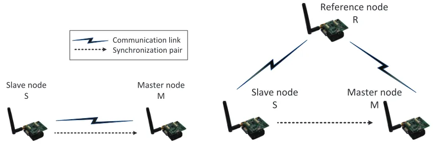
Pairwise synchronization approaches can be classified in two fundamental different schemes based on either receiver measurements or receiver-receiver measurements as shown in Fig. 3.1. The sender-receiver approaches can be further classified in one-way and two-way sender-sender-receiver approaches. In what follows we show how packet transmission in each approach relates to the timing information using the notations we introduced in the previous section.

3.4.1 One-way Sender-Receiver

In this scheme shown in Fig. 3.1(a), the master node periodically broadcasts beacon packets containing its local timestamps every beacon interval ∆TB

M as shown in Fig. 3.2. Once the periodic sending timer

fires at the master node, an APP-layer timestamp Tm,tx,s

M (k) of the kth packet is generated after the

interrupt delay Im,tx,s

M (k) and quantization delay Q m,tx,s

M (k). When available, to remove some of the

sender-side uncertain delays, the MAC-layer timestampT′m,tx,s

M (k) is generated after the sender-OS delay Om,tx,s

M (k) and access delay A m,tx,s

M (k). Once the master transmits the packet out with a transmission

delay Xm,tx,s

M (k), the slave receives the packet after a propagation delay P s,rx,m

S (k) and then forwards

the packet to the upper layers. The receiving MAC-layer timestamp T′s,rx,m

S (k) is generated after the

receiver interrupt delayIs,rx,m

S (k) and quantization delayQ s,rx,m

(29)

Slave node S

Master node M

Communication link Synchronization pair

(a) Sender-Receiver based synchronization

Reference node

R

Slave node

S

Master node

M

(b) Receiver-Receiver based synchronization

Figure 3.1: Pairwise synchronization topologies where a slave node(s) wants to obtain an estimate of a master node’s time: (a) sender-receiver based synchronization, where the slave node directly synchronizes with the master node; (b) receiver-receiver based synchronization, where the slave node synchronizes with the master node with the help of a common reference node.

Ts,rx,m

S (k) is generated after the receiver-OS delayO s,rx,m

S (k). Since the master and slave nodes do not

have the same hardware clock rates with respect to the TAI time scale, relative drift is applied while converting the elapsed time from TAI to the other time scales; for example, Im,tx,s

M (k) = ¯amIUm,tx,s(k)

andOs,rx,m

S (k) = ¯asOs,rU x,m(k). After receiving multiple synchronization beacons, the slave estimates its

relative drift and offset with respect to the master by linear regression. FTSP [4] and PSMV [21] are two examples of one-way sender-receiver synchronization protocols.

3.4.2 Two-way Sender-Receiver

In this scheme depicted in Fig. 3.1(a), the slave node unicasts a synchronization probe packet including local timestamp ˜Ts,tx,m

S (k) to the master node every beacon interval ∆TSB as shown in Fig. 3.3. After

receiving the packet at local timestamp ˜Tm,rx,s

M (k), the master node sends a reply packet back including

its timestamp ˜Tm,tx,s

M (kR) as well as the probe packet’s sending and receiving timestamps, where kR

denotes the kth reply. The slave node then receives the reply at local timestamp ˜Ts,rx,m

S (kR). After

receiving the reply, the slave node can employ linear regression between the average timestamp of the sending probe and receiving reply (i.e., ( ˜Ts,tx,m

S (k) + ˜T s,rx,m

S (kR))/2) and the average timestamp of

receiving probe and sending reply (i.e., ( ˜Tm,rx,s M (k) + ˜T

m,tx,s

M (kR))/2) to estimate the relative drift and

(30)

. . .

Master

t

Slave

t s r m, ,x _{( )}

S k P , , ( ) x mt s M k

I Q_Mmt s, ,x ( )k O_Mmt s, ,x ( )k A_Mm t s, ,x ( )k X_Mmt s, ,x ( )k

, , ( ) x

sr m S k

I Q_Ss r m, ,x ( )kOs r m_S, ,x ( )k

, , ( )

x s r m

S k

x

, , ( )

x m t s

M k

x

' , , ( )

x

s r m

S k

x

' , , ( )

x m t s

M k x B M T D , , ( +1) x mt s M k

I mt s, ,x ( +1)

M k Q B M T D

Ideal beacon generation time

Sender (master node) interrupt delay of thekth beacon Sender quantization delay

Sender OS delay Sender access delay

Sender transmission delay

Sender (master node) APP-layer timestamp

Sender MAC-layer timestamp

Receiver propagation delay Receiver interrupt delay

Receiver quantization delay Receiver OS delay

Receiver APP-layer timestamp Receiver (slave node) MAC-layer timestamp

Sender interrupt delay of thek+1th beacon

Figure 3.2: One-way sender-receiver synchronization timing diagram during the transmission and re-ception of the kth synchronization packet, where the tM aster and tSlave denote the time scales at the

master and slave nodes, respectively.

the relative offset as the difference between the average timestamp of receiving probe and sending reply and the average timestamp of sending probe and receiving reply [5]. TPSN [5] and TSVP [28] are two examples of two-way sender-receiver synchronization protocols.

Master t Slave t , , ( ) x mr s M k P , , ( ) x st m S k I st m, ,x( )

S k Q st m, ,x( )

S k

O st m, ,x( )

S k

A st m, ,x( )

S k X , , ( ) x mr s M k I mr s, ,x( )

M k

Q mr s, ,x( )

M k

O , ,x( ) R

mt s M k

I , ,x( )

R st m M k X , , ( ) x R sr m S k

P , ,x( )

R

sr m S k

I , ,x ( )

R

sr m

S k

Q , ,x ( )

R sr m S k O , , ( ) x R mt s M k

Q , ,x( )

R

mt s

M k

O , ,x( )

R mt s M k A B S T D ' , , ( ) x

s t m

S k x s, , ( ) x t m S k x

' , ,s

( )

x

m r

M k

x , ,s

( )

x

m r

M k

x , ,

(_R)

x

m t s

M kR

x ' , ,

( )

x R

m t s

M k x R ' , , ( ) x R

s r m

S k x R , , ( ) x R

s r m

S k x R

. . .

, , ( +1) x

s t m

S k I B S T D

Sender (slave node) interrupt delay of thekth probe Sender quantization delay

Sender OS delay Sender access delay

Sender APP-layer timestamp of the probe

Sender interrupt delay of thek+1th probe

Receiver (master node) propagation delay Receiver interrupt delay

Sender (slave node) interrupt delay of thekth probe reply Sender quantization delay

Sender OS delay

Sender transmission delay Sender access delay

Receiver (slave node) propagation delay of thekth probe reply Receiver interrupt delay

Receiver APP-layer timestamp Receiver (master node) MAC-layer timestamp of the probe

Sender (master node) APP-layer timestamp of the probe reply

Receiver (slave node) APP-layer timestamp Receiver MAC-layer timestamp of the probe reply Sender MAC-layer timestamp

Sender MAC-layer timestamp

(31)

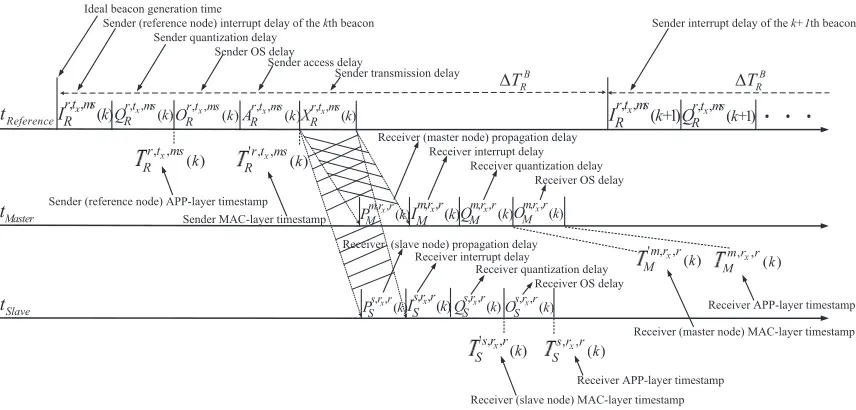
3.4.3 Receiver-Receiver

In this scheme shown in Fig. 3.1(b), the reference node broadcasts a beacon packet every beacon interval ∆TB

R. Although the master and slave nodes experience the same sender-side delays (i.e.,D r,tx,m

R (k) =

Dr,tx,s

R (k), where D∈(I, Q, O, A, P)), the receiver-side delays vary for the two receiving nodes as

they experience different propagation, interrupt, quantization and receiver-OS delays (i.e., in general,

Dm,rx,r

M (k)6=D

s,rx,r

S (k) whereD∈(P, I, Q, O)) as shown in Fig. 3.4. Once receiving multiple

synchroniza-tion beacons from the reference node, the slave node estimates its relative drift and offset with respect to the master by employing linear regression between the local receiving timestamps of the slave and the master’s (i.e., between ˜Ts,rx,r

S (k) and ˜T m,rx,r

M (k)). RBS [19] and CESP [3, 23] are two examples of

receiver-receiver synchronization protocols.

, , ( )

x r t ms

R k

x

, ,

( )

x s r r

S k

x

, ,

( )

x

m r r

M k x B R T D ' , , ( ) x r t ms

R k

x

' , , ( )

x s r r

S k

x

' , ,

( )

x m r r

M k x Master t Slave t Reference t , , ( ) x mr r M k O , , ( ) x

m r r

M k Q , , ( ) x mr r M k I , , ( ) x

m r r

M k

P

, ,

( )

x

s r r

S k

P s r r, ,x ( )

S k

I Q_Ss r r, ,x ( )k s r r, ,x ( )

S k

O

, ,

( )

x

r t ms

R k

O

, ,

( )

x

r t ms

R k

Q r t ms, ,x ( )

R k

A , ,

( )

x r t ms

R k

I r t ms, ,x ( )

R k

X r t ms, ,x ( +1)

. . .

R k

Q , ,

( +1)

x r t ms

R k I B R T D

Sender (reference node) interrupt delay of thekth beacon

Sender quantization delay Sender OS delay

Sender access delay

Sender (reference node) APP-layer timestamp Sender MAC-layer timestamp

Sender interrupt delay of thek+1th beacon

Receiver (master node) propagation delay Receiver interrupt delay

Receiver (slave node) propagation delay Receiver interrupt delay

Receiver APP-layer timestamp Receiver (slave node) MAC-layer timestamp

Receiver APP-layer timestamp

Receiver (master node) MAC-layer timestamp

(32)

Chapter 4

Coefficient Exchange

Synchronization Protocol

In this chapter, Section 4.1 presents the design of CESP protocol. Section 4.2 shows the experimental results of the proposed CESP. The summary of this chapter is shown in Section 4.3.

4.1 CESP Algorithm

In this section, pairwise synchronization using CESP is explained first, followed by an extension for global synchronization and an improved algorithm (CESP-MA) based on moving average coefficients to achieve better synchronization accuracy while still preserving a low communication overhead.

4.1.1 CESP Pairwise Synchronization

Assume there areN sensor nodes scattered in an area, each sensor node with a unique ID number (≥1). A typical receiver-receiver pairwise synchronization topology is shown in Fig. 3.1(b), where sensor node

Rworks as a reference node that periodically broadcasts beacon packets for synchronization, and sensor nodesS, M are receiving nodes where nodeS works as a slave node that wants to synchronize with its master node M by estimating asm and bsm (assuming asm and bsm remain constants for an extended

(33)

Section 4.1.4. For now assume the reference node is already chosen and known to both the master and slave nodes, and that the slave node knows its synchronization master node. Each beacon packet carries a timestamp, which records reference node’s local time when the packet is generated at the application layer. CESP divides the time into synchronization periods and uses information collected in each syn-chronization period to synchronize the clocks at the end of the period. CESP utilizes the timestamps in beacon packets to synchronize each receiving node with a common reference node first, and then ex-changes local synchronization coefficients between receiving nodes for receiver-receiver synchronization. The CESP can be decomposed into the following three phases (also summarized in Algorithms 1-3):

Local Synchronization

To enable synchronization, beaconpackets from reference nodes are broadcasted periodically. The time interval between two consecutive beacon packets is abeacon intervaldenoted as ∆Tb. Asynchronization

periodTsis defined as the time it takes to sendk beacons:

Ts= ∆Tb·k. (4.1)

Each beacon packet includes the ID of the reference node, the time the packet was generated, and a period number (incremented by the reference node at the end of each synchronization period). Each receiving node stores the information in the received beacons (reference node ID, beacon number, syn-chronization period, sending timestamp) and each beacon’s local receiving timestamp in a circular buffer of sizek.

At the end of a synchronization period (detected by the receiving nodes as an increase in the syn-chronization period number), the receiving nodes employ a least square linear regression between the received timestamps and the timestamps in the beacons (similar to the way FTSP [4] works). It is pos-sible that the number of received beacon packetsNr is smaller thank during a synchronization period

(34)

Coefficient Exchange

Once a master node generates its local relative drift and offset estimates with respect to a reference node, a coefficient exchange packet is constructed with the following fields: <src id, ref id, hash code,

ref drift, ref offset>, wheresrc idandref iddenote the node ID of master node and its reference node,

respectively (i.e., nodesM andR in Fig. 3.1(b));hash codeis an integer computed by a hash function with the received beacon numbers as input (i.e., the hashes computed by two receiving nodes match only if they receive the same beacons); ref drif tand ref of f setare the relative drift and offset estimates of master node with respect to the reference node. The master node M then unicasts its coefficient exchange packet to reference nodeR. The reference node broadcasts the received coefficient exchange packets such that the slave node(s) can receive a copy of master node’s local synchronization coefficients. When a slave node receives a broadcast coefficient exchange packet originating at its master, it initiates the receiver-receiver pairwise synchronization phase.

Pairwise Synchronization

To synchronize with a master node receiving from a common reference node, a slave node needs both its own and its master node’s coefficients relative to the common reference node. Denote by ˆasr and ˆbsr

the slave node’s relative drift and offset coefficients with respect to the common reference nodeR and denote by ˆamr and ˆbmr the synchronization coefficients of the master node with respect to the same

reference nodeR. Pairwise synchronization coefficients of the slave node with respect to its master node can be derived as:

ˆ

asm=

ˆ

asr

ˆ

amr

, (4.2)

ˆ

bsm=

ˆ_b_sr₋ˆ_b_mr ˆ

amr

, (4.3)

where ˆasmand ˆbsmare the relative clock drift and offset estimates when a slave node synchronizes to its

master node. We will show in Section 4.2 that when the slave and the master receive different subsets of the beacons from the reference node, sender-side uncertainties (i.e., sender OS and access delays) significantly degrade the accuracy of the synchronization protocol. Therefore, the slave node updates its current estimated relative drift and offset as ˆasm and ˆbsm only if its locally computed hash code

(35)

are used to check if the slave node receives the same copy of beacons as the master node. Different sets of received beacons in the slave and master nodes could result in synchronization inaccuracy when estimating pairwise relative drift and offset due to the effects of different access delays. If the pairwise hash codes do not match, the slave node continues to use the previously computed ˆasm and ˆbsm as its

best estimates of the current relative drift and offset. If MAC-layer timestamping is available, CESP does not require hash codes due to the elimination of sender-side uncertainties.

Algorithm 1: CESP Reference Node Algorithm

Input: Synchronization period (sync period) and beacon interval (beacon int).

Init() begin

beacon num= 0;

sync period num= 0;

set periodic timer (beacon int); end

On Timer Fired() begin

broadcast beacon pkt (beacon num, sync period num, ref timestamp, ref ID);

beacon num++;

if beacon num mod ⌈sync period/beacon int⌉== 0 then

sync period num++;

beacon num= 0; end

On Receive Coefficient Packet() begin

broadcast received coefficient exchange packet; end

4.1.2 Comparison with RBS

(36)

Algorithm 2: CESP Master Node Algorithm

Input: Pairwise synchronization reference node ID (sync ref ID).

Init() begin

curr sync period= 0;

received beacons= []; end

On Receive Beacon() begin

extractbeacon num,sync period num,ref timestamp,ref IDfrom beacon;

if sync ref ID ==ref IDthen /* only process beacons from the assigned reference node */

if curr sync period 6=sync period numthen /* end of current synchronization period */

compute relative drift and offset to reference node and hash code from received beacons; send coefficient exchange packet(master ID, ref ID, master hash, master coef f) to the assigned reference node;

curr sync period=sync period num;

received beacons= [];

store the received beacons in circular buffer: received beacons; end

additional benefit of CESP is that the reference nodes broadcast the received synchronization coefficients from each master node thus enabling pairwise synchronization even when the master and slave are not within each other’s communication range.

4.1.3 CESP with Moving Average Coefficients (CESP-MA)

Moving average is commonly used to smooth short-term fluctuations to achieve a long-term stability [69]. The estimated relative drift and offset can employ moving average to filter out measurement noise to improve estimation. Algorithm 4 shows an improved algorithm named CESP-MA that uses exponentially weighted moving average on the estimated synchronization coefficients to achieve better synchronization accuracy. CESP-MA works the same as CESP regarding reference and master nodes but uses a slightly different approach on computing the newly estimated relative drift and offset regarding slave nodes: the synchronization coefficients are calculated not only based on the newly computed relative drift and offset, but also using the prior estimates as follows:

ˆ

aM A(n) = (1−α)·ˆaM A(n−1) +α·ˆaCESP(n), (4.4)

(37)

Algorithm 3: CESP Slave Node Algorithm

Input: Pairwise synchronization reference node ID (sync ref ID) and master node ID (sync master ID).

Output: The current estimated relative drift and offset with respect to the master node.

Init() begin

curr sync period= 0;

current relative drift and offset (aCESP,bCESP) = [1,0];

end

On Receive Beacon() begin

extractbeacon num,sync period num,ref timestamp,ref IDfrom beacon;

if sync ref ID ==ref IDthen /* only process beacons from the assigned reference node */

if curr sync period 6=sync period numthen /* end of current synchronization period */

compute relative drift and offset to reference node and hash code (slave hash) from received beacons;

curr sync period=sync period num;

store the received beacons in circular buffer: received beacons; end

extractmaster ID, ref ID, master hash,master coef f from synchronization coefficient exchange packet;

if sync ref ID ==ref IDandsync master ID ==master ID then /* only process coefficients from the assigned reference and master nodes */

if slave hash== master hashorcurr sync period == 1 then

calculate new estimated relative drift and offset (new drift, new offset) using (4.2),(4.3); ˆ

aCESP = new drift;

(38)

where ˆaM A(n) and ˆbM A(n) denote the slave’s estimated relative drift and offset to its master at the end

of nth synchronization period of CESP-MA; ˆaM A(n−1) and ˆbM A(n−1) denote the prior estimated

relative drift and offset at the end of (n−1)th synchronization period of CESP-MA; ˆaCESP(n) and

ˆ_b_CESP₍_n_{) denote the relative drift and offset calculated at the end of} _n_{th synchronization period of}

CESP; α and β denote the moving average coefficients for the estimated relative drift and offset of CESP-MA, respectively.

The performance of CESP-MA is improved by using prior estimates rather than restarting from scratch every synchronization period. We will show in the evaluation sections that CESP-MA is not very sensitive to the moving average coefficientsα.

Algorithm 4: CESP-MA Slave Node Algorithm

Input: Pairwise synchronization reference node ID (sync ref ID), master node ID (sync master ID) and moving average coefficients α, β.

Output: The current estimated relative drift and offset at the end ofnth synchronization period.

Init(); /* same as CESP Algorithm 3 */;

On Receive Beacon(); /* same as CESP Algorithm 3 */;

extractmaster ID, ref ID, master hash,master coef f from synchronization coefficient exchange packet;

if sync ref ID ==ref IDandsync master ID ==master ID then /* only process coefficients from the assigned reference and master nodes */

if slave hash== master hashorcurr sync period == 1 then

calculate new estimated relative drift and offset (new drift, new offset) using (4.2),(4.3); if curr sync period == 1 then

ˆ

aCESP−M A= ˆaCESP;

ˆ

bCESP−M A= ˆbCESP;

else ˆ

aCESP−M A(n) = (1−α)·aˆCESP−M A(n−1) +α·ˆaCESP(n);

ˆ

bCESP−M A(n) = (1−β)·ˆbCESP−M A(n−1) +β·ˆbCESP(n);

end

4.1.4 Multihop Network Synchronization

(39)

the synchronization logical graph. To improve CESP multihop synchronization precision, the adaptive clock speed adjustment algorithm proposed in [12] can be employed to show the feasibility of achieving high synchronization accuracy in Fig. 4.10.

The synchronization graph [19] is a subset of the physical graph in sender-receiver based synchro-nization protocols such as FTSP, TPSN and TinySync. However, the two are not directly related in the case of receiver-receiver based synchronization schemes such as RBS and CESP. For example, Fig. 4.1(a) shows an example of a physical graph. Figures 4.1(b) and 4.1(c) show the corresponding synchronization logical graphs for CESP and RBS, respectively, if RBS does not enable reference node forwarding of local timestamps from master nodes. Finally, Figs 4.1(d) and 4.1(e) show a spanning tree based on synchro-nization logical graph such that each node in the network knows its reference node and its master node. Each node can work as a master, a slave, a reference node, or a combination of these roles, and each pair of master and slave nodes could have multiple choices for their reference node. In the example shown in Fig. 4.1, CESP enables pairwise synchronization even when pairwise receiving nodes are not within each other’s communication range by using the reference node to broadcast synchronization coefficients such that slave node 5 can still synchronize with one of the master nodes 1,2,4 via the help of reference node 3 (whereas slave node 5 is unsynchronized in RBS), and the number of hops needed for network wide synchronization is reduced: RBS has to use two hops to synchronize the network, whereas CESP can use only a single hop. If RBS enables reference nodes to forward local timestamps of master nodes, the synchronization logical graph of RBS is identical to the one of CESP.

4.2 Experimental Results and Analysis

To test protocols’ performance in a realistic testbed, we conduct experiments on TelosB [13] platform using TinyOS [71] version 2.1.2 to measure synchronization error and the number of synchronization packets sent and received using CESP and CESP-MA in comparison with other well-known synchro-nization protocols.

4.2.1 Experimental Setup

(40)

3

4 5

1

2

(a)

1

2 3

4 5

<1or4>

<3> <2>

<3>

<3> <2>

<3> < < <

<2or3>

(b)

1

2 3

4 5

<1or4>

<2> <3>

<3> <2>

(c)

1

2 3 4 5

<3> <2> <3> <3>

(d)

1

2

4

3

5

<3> <2>

<3>

(e)

Figure 4.1: Example of a multihop network topology using CESP and RBS: (a) the physical graph specifying physical connectivity; (b) CESP synchronization logical graph with dash line drawn between nodes that can receive from a common reference node (marked in<>on each edge), and therefore can synchronize their clocks to each other; (c) RBS synchronization logical graph if RBS does not enable reference node to forward local timestamps of master node; (d) CESP synchronization spanning tree corresponding to (b) with node 1 as the root; (e) RBS synchronization spanning tree corresponding to (c) with node 1 as the root.

Overview of TelosB and TinyOS

The core processing unit of TelosB is Texas Instruments MSP430 microcontroller which uses an external 32KHz crystal oscillator with tolerance of 5-30ppm as the clock source of internal digitally controlled oscillator (DCO) that may operate up to 8MHz. TinyOS is an operating system designed for low-power wireless embedded systems in a structure of components and interfaces [71]. The Timer component provides timing precision of milliseconds, a cycle of a 32kHz clock or microseconds. In the experiment, reference nodes periodically broadcast beacon packets triggered by milliseconds timer. All the received and transmitted packets’ local timestamps are generated by theCounter component that handles timer overflow and uses a microseconds timer to provide high precision timestamping. MSP430 can enable MAC-layer timestamping using the start-of-frame delimiter (SFD) interrupt supported by the CC2420 radio stack, which eliminates sender OS, receiver OS and access delays.

Sensor Nodes Configuration

Clock Synchronization in Wireless Sensor Networks: Performance Analysis and Protocol Design.

ABSTRACT

DEDICATION

BIOGRAPHY

ACKNOWLEDGEMENTS

TABLE OF CONTENTS

LIST OF TABLES

LIST OF FIGURES

Chapter 1

Introduction

1.1

Overview

1.1.1

Wireless Sensor Networks

1.1.2