PARK, HEE MUN. Use of Falling Weight Deflectometer Multi-Load Level Data for
Pavement Strength Estimation. (Under the direction of Y. Richard, Kim).
The objective of this study is to describe a mechanistic-empirical approach to
developing an analysis method for assessing pavement layer conditions and estimating
the remaining life of flexible pavements using multi-load level Falling Weight
Deflectometer (FWD) deflections. A dynamic finite element program, incorporating a
stress-dependent soil model, was developed to generate the synthetic deflection database.
Based on this synthetic database, the relationships between surface deflections and
critical pavement responses, such as stresses and strains in each individual layer, have
been established.
A condition assessment procedure for pavement layers using multi-load level
FWD deflections is presented in this study. The results indicate that the proposed
procedure can estimate the base and subgrade layer conditions. However, large
variations were observed in the relationships between the DBCI and dεsg values and the subgrade CBR values for aggregate base pavements. A FWD test with a load of 53 kN or
less does not result in any apparent nonlinear behavior of the subgrade in aggregate base
pavements. With regard to the condition assessment of the asphalt concrete (AC) layer,
the AC layer modulus and the tensile strain at the bottom of the AC layer are found to be
better indicators than the deflection basin parameter.
The procedures for performance prediction of fatigue cracking and rutting are
developed for flexible pavements. The drastically increasing trend in fatigue cracking
Predicted rut depths using both single and multi-load level deflections show good
agreement with measured rut depths over a wide range of rutting potential. However, the
procedure using single load level deflections consistently underpredicts the rut depths.
This observation demonstrates that the rutting prediction procedure using multi-load level
deflections can estimate an excessive level of rutting quite well and, thus, improve the
FOR PAVEMENT STRENGTH ESTIMATION
by
HEE MUN PARK
A dissertation submitted to the Graduate Faculty of North Carolina State University
in partial fulfillment of the requirements for the Degree of
Doctor of Philosophy
DEPARTMENT OF CIVIL ENGINEERING
Raleigh
2001
APPROVED BY:
BIOGRAPHY
Hee Mun Park was born on Jan 10, 1971 in Kwangju, Korea. He received his B.S.
degree in Civil Engineering in 1996 from Hanyang University in Seoul. In 1998, he
received M.E. in Civil Engineering from Texas A&M University at College Station in
Texas. From August 1998, he began to work on his Doctor of Philosophy degree in Civil
Engineering at North Carolina State University, under the direction of Dr. Y. Richard
ACKNOWLEDGEMENTS
I would like to express my gratitude to my advisor Dr. Y. Richard Kim for all the
encouragement, help, and guidance that he has given to me during the course of my
graduate study.
I would also like to thank Dr. Roy H. Borden, Dr. S. Ranji Ranjithan , Dr. Murthy N.
Guddati for their advices and concerns in helping me to accelerate the growth of my
doctoral studies.
My thank must go to some of my fellow graduate students for all sorts of help and
friendship. These include Bing Xu and Sungho Mun.
This research was sponsored by the North Carolina Department of Transportation
(NCDOT). I would like to thank the Pavement Management Unit of NCDOT for their
efforts in performing FWD tests and data collections.
Thanks are given to my wife, Hyekyoung Yang, my parents, and family for their love,
TABLE OF CONTENTS
LIST OF TABLES ………...……….vi
LIST OF FIGURES ………..vii
1 INTRODUCTION ...……….1
1.1 Background ………..…………..………1
1.2 Objectives and Scope ……….………...3
2 LITERATURE REVIEW ………5
2.1 Falling Weight Deflectometer (FWD) ………5
2.2 Dynamic Cone Penetrometer (DCP) ………7
2.3 Stress-State Dependent Soil Model ………8
3 FORWARD MODELING OF PAVEMENTS ……….……….…11
3.1 General Description of Finite Element Model ………..11
3.2 Dynamic Finite Element Model ………..………13
3.3 Verification of Finite Element Model ………..………15
4 DEVELOPMENT OF PAVEMENT RESPONSE MODELS …………..25
4.1 Existing Pavement Response Models ………..…26
4.1.1 Fatigue Cracking ………..…26
4.1.2 Rutting ………..28
4.2 Synthetic Pavement Response Databases ………..29
4.3 Parametric Sensitivity Analysis of Pavement Responses ………..30
4.4 Pavement Response Model for Fatigue Cracking Potential …………..32
4.5 Pavement Response Model for Rutting Potential ………..36
5 DEVELOPMENT OF TEMPERATURE CORRECTION FACTORS …..40
5.1 Selection of Pavement Sections ………..41
5.2 Synthetic Pavement Response Databases ………..42
5.3 Mid-Depth Temperature Prediction ………..43
5.4 Effect of Load Level on Temperature Correction of FWD Deflections …..44
5.5 The Effective Radial Distance for Temperature Correction of FWD Deflections ………..45
5.6 Temperature Correction of Deflections at Radial Offset Distance …..48
6 CONDITION ASSESSMENT OF PAVEMENT LAYERS USING
MULTI-LOAD LEVEL FWD DEFLECTIONS ………..………56
6.1 Full Depth Pavements ………..………56
6.1.1 Subgrade …………...………...56
6.2 Aggregate Base Pavements ………..64
6.2.1 AC Layer ………..64
6.2.2 Base Layer ………..74
6.2.3 Subgrade ………..79
6.2.4 Validation of Condition Assessment Procedure Using NCDOT Data ………..85
6.2.5 Effect of Load Level on Nonlinear Behavior of a Pavement Structure ………..89
6.3 Summary ………..97
7 DEVELOPMENT OF MULTI-LOAD LEVEL DEFLECTION ANALYSIS METHODS ………..99
7.1 Pavement Performance Model ………..99
7.1.1 Fatigue Cracking ………..99
7.1.2 Permanent Deformation ………101
7.2 Remaining Life Prediction Method ………102
7.2.1 Cumulative Damage Concept ………104
7.2.2 Traffic Consideration ………108
7.2.3 Performance Prediction for Fatigue Cracking ………109
7.2.4 Performance Prediction for Rutting ………118
7.3 Summary ………113
8 CONCLUSIONS AND RECOMMENDATIONS ………139
8.1 Conclusions………...139
8.2 Recommendations……….140
LIST OF TABLES
Table 3.1. Layer Thicknesses and Material Properties for the Linear Elastic Analysis .. 16
Table 3.2. The Coefficient of K-θ Model for the Nonlinear Elastic Analysis ... 16
Table 3.3. Layer Thicknesses and Material Properties Used in Dynamic Finite Element Analysis ... 21
Table 4.1. SSR Design Criteria during Critical Period (after Thompson, 1989) ... 29
Table 4.2. Nonlinear Elastic Synthetic Database Structures ... 30
Table 4.3. Deflection Basin Parameters ... 31
Table 4.4. Parametric Analysis Results for Full-Depth Pavements ... 31
Table 4.5. Parametric Analysis Results for Aggregate Base Pavements ... 32
Table 5.1. Pavement Test Sections... 42
Table 5.2. Results of T Test ... 44
Table 5.3. C0-value for Each Region and the State... 50
Table 6.1. Results of Coring for Full Depth Pavements ... 60
Table 6.2. Criteria for Poor Subgrade in Full Depth Pavements... 61
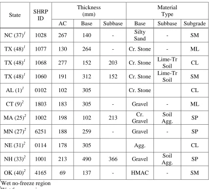
Table 6.3. Characteristics of Pavement Test Sections in LTPP Data ... 65
Table 6.4. Area with Fatigue Cracking in LTPP Test Sections ... 67
Table 6.5. A Summary of Coring and DCP Testing for Aggregate Base Pavements... 75
Table 6.6. Criteria for Poor Base Layer in Aggregate Base Pavements ... 76
Table 6.7. Criteria for Poor Subgrade Layer in Aggregate Base Pavements ... 81
Table 6.8. Results of Visual Distress Survey in NCDOT Test Sections... 85
Table 7.1. Typical Permanent Deformation Parameters for Flexible Pavement Materials (after Bonaquist, 1996)... 102
Table 7.2. Calculation of Damage due to Mixed Load Groups ... 106
Table 7.3. Magnitude of Distress Related to Cracking for Each Category... 111
Table 7.4. The VESYS Rutting Parameters (after Park, 2000, and Kenis, 1997)... 119
Table 7.5. Magnitude of Distress Related to Rutting for Each Category... 123
Table 7.6. Measured Rut Depths for LTPP Test Sections ... 123
LIST OF FIGURES
Figure 1.1. Different effects of multi-load levels on deflections from pavements with
different strengths... 3
Figure 2.1. Pavement responses under FWD loading. ... 6
Figure 2.2. A typical deflection basin. ... 6
Figure 2.3. A schematic of the dynamic cone penetrometer. ... 7
Figure 3.1. Surface deflections in a two-layer pavement system... 17
Figure 3.2. Surface deflections in a three-layer pavement system... 17
Figure 3.3. Surface deflections in the nonlinear analysis... 19
Figure 3.4. Variations of vertical stress... 19
Figure 3.5. Variations of horizontal stress. ... 20
Figure 3.6. Stress-dependent modulus distribution... 20
Figure 3.7. A schematic of sample specimen... 22
Figure 3.8. Comparison of displacement-time histories obtained from NCPAVE and ABAQUS (2x2 mesh). ... 22
Figure 3.9. Displacement-time histories in 100x100 mesh size specimen... 23
Figure 3.10. Displacement - time histories of a pavement structure under FWD loading. ... 23
Figure 3.11. Computed deflection basin. ... 24
Figure 4.1. Area Under Pavement Profile. ... 27
Figure 4.2. The relationship between the tensile strain at the bottom of the AC layer and the BDI (40 kN load level)... 34
Figure 4.3. The relationship between the tensile strain at the bottom of the AC layer and the AUPP (40 kN load level)... 34
Figure 4.4. Comparison of εac predictions from the BDI and AUPP for asphalt concrete pavements... 35
Figure 4.5. The relationship between the compressive strain on the top of the base layer and the BDI for aggregate base pavements (40 kN load level)... 37
Figure 4.6. The relationship between the compressive strain on the top of the subgrade and the BDI for full depth pavements (40 kN load level). ... 38
Figure 4.7. The relationship between the compressive strain on the top of the subgrade and the BCI for aggregate base pavements (40 kN load level). ... 39
Figure 5.1. Predicted mid-depth temperature versus measured mid-depth temperature.. 43
Figure 5.2. Effect of multi load level on temperature-dependency of deflections for US 264... 45
Figure 5.3. Deflection versus mid-depth temperature for: (a) US 264; (b) US 17... 47
Figure 5.4. Effective radial distance versus AC layer thickness for all pavement sites... 48
Figure 5.6. NCDOT corrected center deflection versus mid-depth temperature for: (a) eastern region; (b) central region; (c) western region. ... 53 Figure 5.7. LTPP corrected center deflection versus mid-depth temperature for: (a) eastern region; (b) central region; (c) western region. ... 54 Figure 5.8. The distribution of n value for LTPP temperature correction procedure. ... 55
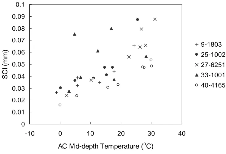
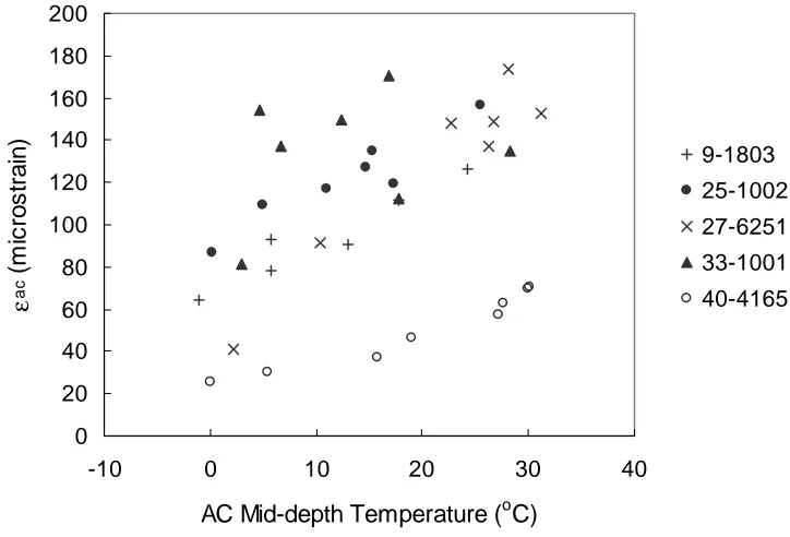
Figure 6.1. Adjusted BDI as a subgrade condition indicator for full depth pavements. .. 62 Figure 6.2. Adjusted DBDI as a subgrade condition indicator for full depth pavements.62 Figure 6.3. Adjusted εsg as a subgrade condition indicator for full depth pavements... 63 Figure 6.4. Adjusted dεsg as a subgrade condition indicator for full depth pavements.... 63 Figure 6.5. SCI versus AC mid-depth temperature for LTPP test sections in a wet no-freeze region. ... 69 Figure 6.6. SCI versus AC mid-depth temperature for LTPP test sections in a wet freeze region... 69 Figure 6.7. DSCI versus AC mid-depth temperature for LTPP test sections in a wet no-freeze region. ... 70 Figure 6.8. DSCI versus AC mid-depth temperature for LTPP test sections in a wet freeze region. ... 70 Figure 6.9. εac versus AC mid-depth temperature for LTPP test sections in a wet
no-freeze region. ... 71 Figure 6.10. εac versus AC mid-depth temperature for LTPP test sections in a wet freeze
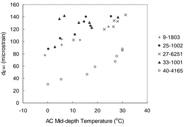
region... 71 Figure 6.11. dεac versus AC mid-depth temperature for LTPP test sections in a wet
no-freeze region. ... 72 Figure 6.12. dεac versus AC mid-depth temperature for LTPP test sections in a wet freeze
region... 72 Figure 6.13. Eac versus AC mid-depth temperature for LTPP test sections in a wet no-freeze region. ... 73 Figure 6. 14. Eac versus AC mid-depth temperature for LTPP test sections in wet no-freeze region. ... 73 Figure 6.15. Determination of base layer thickness for the SR 2026 section. ... 75 Figure 6.16. Adjusted BDI as a base condition indicator for aggregate base pavements.77 Figure 6.17. Adjusted DBDI as a base condition indicator for aggregate base pavements.
... 77 Figure 6.18. Adjusted εabc as a base condition indicator for aggregate base pavements. 78 Figure 6.19. Adjusted dεabc as a base condition indicator for aggregate base pavements.
... 78 Figure 6.20. Adjusted BCI as a subgrade condition indicator for aggregate base
pavements... 82 Figure 6.21. Adjusted DBCI as a subgrade condition indicator for aggregate base
pavements... 82 Figure 6.22. Adjusted εsg as a subgrade condition indicator for aggregate base
pavements... 83 Figure 6.23. Adjusted dεsg as a subgrade condition indicator for aggregate base
Figure 6.25. Esg as a subgrade condition indicator for aggregate base pavements. ... 84
Figure 6.26. Magnitudes of εac for the US 264, US 74, and US 421 sections in 1995 and 2001... 86
Figure 6.27. Magnitudes of εabc for the US 264 and US 74 sections in 1995 and 2001. . 87
Figure 6.28. Magnitudes of εsg for the US 264, US 74, and US 421 sections in 1995 and 2001... 87
Figure 6.29. Percent of increase in εac between 1995 and 2001 for the US 264, US 74, and US 421 sections. ... 88
Figure 6.30. Percent of increase in εabc between 1995 and 2001 for the US 264 and US 74 sections. ... 88
Figure 6.31. Percent of increase in εsg between 1995 and 2001 for the US 264, US 74, and US 421 sections. ... 89
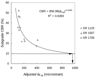
Figure 6. 32. Normalized deflections at SR 1125. ... 91
Figure 6.33. Normalized deflections at SR 1706. ... 91
Figure 6.34. Subgrade CBR value versus deflection ratio for full depth pavements. ... 92
Figure 6.35. Base CBR value versus deflection ratio for aggregate base pavements. ... 92
Figure 6.36. Subgrade CBR value versus deflection ratio for aggregate base pavements. ... 93
Figure 6.37. Deflection ratio versus AC mid-depth temperature for pavements with a gravel base layer... 95
Figure 6.38. Deflection ratio versus AC mid-depth temperature for pavements with a crushed stone base layer... 95
Figure 6.39. Deflection ratio versus AC mid-depth temperature for pavements with a HMAC base layer... 96
Figure 6.40. Effect of subgrade soil type on nonlinear behavior of a pavement structure. ... 96
Figure 6.41. The flow chart of the procedure for assessment of the pavement layer conditions for aggregate base pavements... 98
Figure 7.1. Conceptual flowchart of the multi-load level data analysis method for remaining life prediction. ... 107
Figure 7.2. Change in area with fatigue cracking measured for pavement with excessive levels of fatigue cracking. ... 112
Figure 7.3. Change in area with fatigue cracking measured for pavement with nominal and moderate levels of fatigue cracking... 112
Figure 7.4. Relationship between area with fatigue cracking versus annual precipitation for LTPP test sections. ... 113
Figure 7.5. Predicted and measured damage ratios due to fatigue cracking for the 37-1027 section (wet no freeze region). ... 114
Figure 7.6. Predicted and measured damage ratios due to fatigue cracking for the 48-1068 section (wet no freeze region). ... 114
Figure 7.7. Predicted and measured damage ratios due to fatigue cracking for the 25-1002 section (wet freeze region). ... 115
Figure 7.9. Predicted and measured damage ratios due to fatigue cracking for the
48-1077 section (wet no freeze region). ... 116
Figure 7.10. Predicted and measured damage ratios due to fatigue cracking for the 48-1060 section (wet no freeze region). ... 116
Figure 7.11. Predicted and measured damage ratios due to fatigue cracking for the 9-1803 section (wet freeze region). ... 117
Figure 7.12. Predicted and measured damage ratios due to fatigue cracking for the 27-6251 section (wet freeze region). ... 117
Figure 7.13. Predicted and measured damage ratios due to fatigue cracking for the 40-4165 section (wet freeze region). ... 118
Figure 7.14. Change in AC mid-depth temperatures recorded in spring/summer season from the 48-1060 section... 121
Figure 7.15. Change in AC mid-depth temperatures recorded in spring/summer season from the 48-1060 section... 121
Figure 7.16. Predicted rut depths using the deflections at monthly and average spring/summer AC mid-depth temperatures for the 48-1060 section. ... 122
Figure 7.17. Predicted rut depths using the deflections at monthly and average spring/summer AC mid-depth temperatures for the 48-1060 section. ... 122
Figure 7.18. Predicted and measured total rut depths for the 37-1028 section. ... 125
Figure 7.19. Predicted and measured total rut depths for the 48-1077 section. ... 126
Figure 7.20. Predicted and measured total rut depths for the 48-1068 section. ... 126
Figure 7.21. Predicted and measured total rut depths for the 48-1060 section. ... 127
Figure 7.22. Predicted and measured total rut depths for the 9-1803 section. ... 127
Figure 7.23. Predicted and measured total rut depths for the 25-1002 section. ... 128
Figure 7.24. Predicted and measured total rut depths for the 27-6251 section. ... 128
Figure 7.25. Predicted and measured total rut depths for the 33-1001 section. ... 129
Figure 7.26. Predicted and measured total rut depths for the 40-4165 section. ... 129
Figure 7.27. Comparison of predicted and measured rut depths for the LTPP test sections (single-load level)... 130
Figure 7.28. Comparison of predicted and measured rut depths for the LTPP test sections (multi-load level)... 130
Figure 7.29. Predicted layer rut depths for the 37-1018 section. ... 131
Figure 7.30. Predicted layer rut depths for the 48-1068 section. ... 131
Figure 7.31. Predicted layer rut depths for the 48-1077 section. ... 132
Figure 7.32. Predicted layer rut depths for the 48-1060 section. ... 132
Figure 7.33. Flow chart for the remaining life prediction procedure for fatigue cracking. ... 135
Figure 7.34. Flow chart for the remaining life prediction procedure for rutting... 136
Figure 7.35. The worksheet for the calculation of the damage ratios due to fatigue cracking for the 38-1018 section... 137
CHAPTER 1
INTRODUCTION
1.1 Background
The Falling Weight Deflectometer (FWD) is an excellent device for evaluating the
structural capacity of pavements in service for rehabilitation designs. Because the FWD
test is easy to operate and simulates traffic loading quite well, many state highway
agencies utilize it widely for assessing pavement conditions.
Generally, surface deflections obtained from FWD testing have been used to
backcalculate in situ material properties using an appropriate analysis technique, or to
predict the pavement responses and then determine the strength and remaining life of the
existing pavement. The typical testing program consists of three drops of the FWD, each
with a load of approximately 40 kN although the FWD is capable of imparting multiple
load levels ranging from about 13 kN to about 71 kN, with little additional effort in
operation.
Multi-load level deflection data could result in significant enhancement of
pavement engineers’ ability to estimate the strength and remaining life of pavements. To
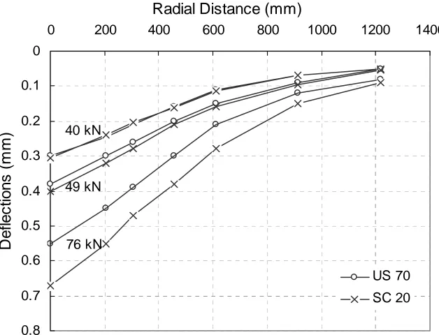
illustrate this point, deflection data under multi-load levels are plotted in Figure 1.1 for
US 70 section (140 mm thick AC layer and 279 mm thick aggregate base) and Section 20
(229 mm thick AC full depth) of US 421. At the time of FWD testing, the US 70 section
was one year old and in good condition, whereas some surface cracks were visible in US
remaining lives. However, the deflection basins of these two pavements under a 40 kN
load were identical. Using the current method based on single-load level (40 kN) data
would result in the same overlay thickness being used for both pavements in spite of their
different strengths and conditions.
The effect of these different strengths of these two pavements becomes evident
when multi-load level data are compared. As shown in Figure 1.1, Section 20 underwent
a greater increase in deflections as the load level increased than US 70 section did. It is
well known that the elastic moduli of unbound materials are stress dependent. When a 40
kN load is used in FWD testing, the resulting stress and strain levels are low enough to
neglect the errors associated with using a stress dependent material model. However, the
analysis of higher load level deflections requires consideration of the nonlinear behavior
of materials. The nonlinear behavior of pavement material induced by multi-load levels
necessitates the use of the finite element method with a stress dependent material model.
It seems clear that this added information would provide another dimension in our
pavement analysis and would improve our knowledge of the relative urgency of various
pavement rehabilitation projects. Although this information can be obtained at no
additional cost in terms of testing time, traffic control requirements for field
investigations, and changes to the equipment, the lack of a reliable analysis method of
multi-load level data prohibits pavement engineers from taking advantage of this readily
Figure 1.1. Different effects of multi-load levels on deflections from pavements with different strengths.
1.2 Objectives
and
Scope
The objective of this study is to describe a mechanistic-empirical approach to developing
an analysis method for assessing pavement layer conditions and estimating the remaining
life of asphalt concrete pavements using multi-load level FWD deflections. The static
and dynamic finite element programs incorporating a stress dependent soil model were
developed to generate the synthetic deflection database. Based on this synthetic database,
the relationships between surface deflections and critical pavement responses, such as
stresses and strains in each individual layer (Pavement Response Models), have been
established. Pavement response models and field databases such as coring, destructive
testing, and visual distress surveys were employed to develop relationships between
40 kN
49 kN
76 kN 0
0.1
0.2
0.3
0.4
0.5
0.6
0.7
0.8
0 200 400 600 800 1000 1200 1400
Radial Distance (mm)
D
e
flec
ti
ons
(
m
m
)
critical pavement responses and pavement strength or performance (Pavement
Performance Models).
Since the performance and the state of stress of asphalt concrete pavements over a
cement-treated base or a Portland cement concrete (PCC) slab are quite different from
those of other asphalt concrete pavements, the scope of this study is limited to full-depth
asphalt concrete pavement and asphalt concrete pavement with an aggregate base course.
Pavement performance characteristics to be investigated in this study include load-related
CHAPTER 2
LITERATURE REVIEW
2.1
Falling Weight Deflectometer (FWD)
The FWD is an example of nondestructive testing equipment that has been widely used
for evaluating the structural capacity and integrity of existing pavements. The FWD test
is performed by dropping a hydraulically lifted weight on top of a circular plate with a
rubber damper that allows uniform distribution of the load on the loading plate. The
impact load has a magnitude ranging from 7 kN to 120 kN with a duration of
approximately 30 ms.
Surface deflections in a pavement structure are measured using a series of
geophones at different offset distances from the center of the loading plate. Figure 2.1
shows the transient responses recorded under FWD loading. Although transient
responses provide more information about pavement analysis, the use of transient data is
too complicated for this analysis. Therefore, only peak deflections obtained from
Figure 2.1. Pavement responses under FWD loading.
Figure 2.2. A typical deflection basin. Deflection Basin Geophone
FWD Load
-100 0 100 200 300 400 500 600
0 0.01 0.02 0.03 0.04 0.05 0.06
Time (sec)
F
W
D
L
oad (
k
P
a
)
-0.1 0 0.1 0.2 0.3 0.4 0.5 0.6 0.7 0.8 0.9 1
S
u
rf
ace
D
e
flect
ion
(
m
m
)
2.2
Dynamic Cone Penetrometer (DCP)
The Dynamic Cone Penetrometer has been widely used to evaluate the structural integrity
of the pavement base and subgrade layers. It is based on the principle of the bearing
capacity failure of a foundation that develops a shear failure zone (Sowers et al., 1966).
Penetration depth per blow is used to estimate the California Bearing Ratio (CBR) value
of the base and subgrade materials and to estimate the strength characteristics of these
materials. The DCP also provides an accurate reading of the thickness of the layers,
which is one of the most critical parameters for analyzing a pavement structure. A
schematic of the dynamic cone penetrometer is shown in Figure 2.3.
Figure 2.3. A schematic of the dynamic cone penetrometer.
Temp ered Cone M easuring Tap e
Handle
Hammer (M ass = 8 kg)
2.3
Stress-State Dependent Soil Model
The resilient modulus in granular material has been known to be stress-state dependent
(Hicks and Monismith, 1971). The K-θ model has been the most popular model for representing the behavior of granular material. The resilient modulus can be expressed
by:
2
1 K
r K
M = θ (2.1)
where
Mr = the resilient modulus,
θ = the sum of principal stresses, and
K1, K2 = material parameters.
The material parameters, K1 and K2, are determined from the repeated triaxial
loading test results. However, the predicted results using the K-θ model are inaccurate because the model neglects the effect of shear stress on the resilient modulus. May and
Witczak (1981) considered the effect of shear stress in estimating the granular material
modulus to describe the nonlinear soil behavior under various loading conditions.
The contour model proposed by Brown and Pappin (1981) expresses the shear and
volumetric stress-strain relations for granular materials using the stress path to simulate
the actual pavement conditions. Due to the complexity of the contour model, it is
difficult to use as a practical model in characterizing granular material. Brown and
Pappin also focused on the importance of effective stress which is caused by pore
pressure in partially or totally saturated materials.
Uzan (1985) proposed the modified stress-state dependent model, known as the
octahedral shear stress. It can account for the stress hardening and softening behavior of
soils. The universal soil model is shown as follows:
3 2
1
K
a oct K
a a r
P P
P K M
= θ τ (2.2)
where
Pa = atmosphere pressure,
τoct = the octahedral shear stress, and K1, K2, K3 = regression parameters.
According to the Witczak and Uzan (1988) study, the universal soil model is
applicable to a wide range of unbound materials having both c and φ properties. As a result of a comparison of the measured to the predicted modulus of granular material, the
universal soil model improved the accuracy of the prediction of the resilient modulus
significantly. In the case of fine-grained soils, it is recommended to use this model in
which the test data have a series of confining pressure.
Tutumluer and Thompson (1997) proposed a cross-anisotropic model to predict
the vertical, horizontal, and shear modulus of granular base materials. Unlike the
isotropic elastic model, the nonlinear anisotropic model is able to show the variations of
the vertical and horizontal moduli of the base materials. Tutumluer and Thompson
concluded that the horizontal modulus is lower than the vertical modulus, and the tensile
stresses at the bottom of the base can be reduced drastically compared to the high tensile
stress in isotropic elastic programs.
The resilient modulus of fine-grained soils is usually dependent on the deviator
decreases with the increase in deviator stress. The degree of moisture content affects the
resilient modulus of fine-grained soils more significantly than that of granular soils
(Thadkamalla and George, 1992).
The bilinear model based on the repeated axial load test shows that the resilient
modulus drastically decreases as the deviator stress increases to breakpoint, and then
slightly decreases. This breakpoint enables one to characterize the type of subgrade soil
and indicate the material responses from the loading condition (Thompson and Elliot,
1985).
As a simple model, the power model was proposed to predict stress-softening
behavior for fine-grained soils:
2
1 K d
r K
M = σ (2.3)
where
σd = the deviatoric stress.
The following model is considered an improvement of the power model, applying both
the deviator stress and confining pressure (P0)for prediction of the resilient modulus (Brown and Loach, 1987).
2
1
K
d o d r
P K
M
=
σ
CHAPTER 3
FORWARD MODELING OF PAVEMENTS
3.1
General Description of the Finite Element Model
The two-dimensional finite element program, NCPAVE, was developed to compute
pavement responses under static and dynamic loading. It considers the pavement as an
axisymmetric solid of revolution and divides it into a set of finite elements connected at
four nodal points. It is capable of automatically generating a finite element mesh for the
analysis of a pavement structure and accommodating the stress-dependent soil model in
the base and subgrade layer.
NCPAVE generates the mesh for the area around the FWD loading plate using
finer elements with a 12.7 mm spacing in the radial direction. The elements become
coarser laterally and vertically away from the load center. The mesh in the vertical
direction is designed to match typical pavement layer thicknesses. A stiff layer with a
modulus of 27,580 MPa was located at the bottom of the subgrade. These combinations
result in a finite element mesh of about 2,500 nodes and 2,200 elements for a typical
flexible pavement structure.
The nodal points at the bottom boundary are fixed whereas those on the right
boundary are constrained from moving in the radial direction. The nodal points on the
centerline are designed to move only vertically because of the axisymmetric nature of the
The program output consists of radial and axial displacements at each of the nodal
points and the state of stress and strain at the centroid of each element. Quadrilateral
stresses are calculated as the average value of the stresses at the four nodal points.
In the finite element analysis, a pavement structure was divided into four groups:
surface layer, base layer, subgrade layer, and stiff layer. Although the behavior of asphalt
concrete is time and temperature dependent, it is assumed to be an elastic material for this
study. To account for the nonlinear behavior of the base and subgrade materials, Uzan’s
universal soil model is incorporated into the program using the following equation:
3 2
1
K
a d K
a a r
P P
P K M
= θ σ (3.1)
where
θ = the sum of the principal stresses,
σd = the applied deviator stress, Pa = atmosphere pressure, and K1, K2, K3 = regression constants.
Uzan’s model is expressed in terms of both deviator and bulk stresses and,
therefore, accounts for the effect of shear stress on the resilient modulus. For static
analysis, an iterative procedure is used to calculate the stress-dependent modulus in each
element of the unbound layers. Convergence is dependent on the difference between the
new and old moduli values. A 2% of difference between the new and old modulus in
each step is acceptable as a convergence criterion. To simulate the state of stress in the
field more accurately, the initial geostatic stress is calculated for each element in the
unit weight used in this program are 22.8 kN/m3 for granular materials, and 19.6 kN/m3
for fine-grained soils.
3.2
Dynamic Finite Element Model
The dynamic nature of the FWD test is one of the most important factors affecting the
pavement responses. Due to the inertia effect on a pavement system, the responses
computed using the static finite element method are different from those measured from
FWD testing. Mamlouk (1987) presented a computer program capable of considering the
inertia effect and also indicated that this effect is most significant when a shallow stiff
layer or frozen subgrade is encountered.
The equilibrium equation for the linear dynamic response of finite elements is as
follows:
R KU U C U
M DD+ D + = (3.2)
where
M, C, and K = the mass, damping, and stiffness matrices;
U, Uand U = the displacement, velocity, and acceleration; and,
R = the external load.
To investigate the dynamic responses of a pavement structure to dynamic loading,
the dynamic equilibrium equation is solved using the explicit integration scheme in which
the displacement at time t+∆t is directly solved in terms of previous displacement and the dynamic equilibrium condition established at time t. As an explicit integration scheme,
the central difference method was implemented in this program based on the following
(
t t t t t)
t U U U tU −∆ − + +∆
∆
= 12 2
(3.3)
(
t t t t)
t
U U
t
U +∆ − −∆
∆ =
2 1
(3.4)
Substituting Equations 3.3 and 3.4 into 3.2, one can obtain:
t t t t t t U C t M t U M t K R U C t M t ∆ − ∆ + ∆ − ∆ − ∆ − − = ∆ +
∆ 2 )
1 1 ( ) 2 ( ) 2 1 1
( 2 2 2 (3.5)
From this equation, one can solve for displacement at t+∆t. The following summarizes the time integration scheme using the central difference method (Bathe, 1982).
A. Initial calculations:
1. Form stiffness matrix, mass matrix, and damping matrix.
2. Initialize U0, U0, and U0.
3. Select time step ∆t.
4. Calculate integration constants:
2 0 1 t a ∆ = ; t a ∆ = 2 1
1 ; a2 =2a0;
2 3
1 a
a =
5. Calculate U−∆t =U0 −∆tU0 +a3U0.
6. Form effective mass matrix Mˆ =a0M +a1C. B. For each time step:
1. Calculate effective loads at time t:
t t t t t U C a M a U M a K R
Rˆ = −( − 2 ) −( 0 − 1 ) −∆ 2. Solve for displacements at time t+∆t:
t t t
R U
Mˆ +∆ = ˆ
(
t t t t t)
tU U U
a
U = 0 −∆ −2 + +∆
(
t t t t)
t
U U
a
U = 1 +∆ − −∆
An important consideration in using the central difference method is that it
requires a small time step to ensure stability of the solution. The critical time step is
expressed as:
πmin
T tcr =
∆ (3.6)
where
Tmin = the smallest natural period of the system.
Material damping of 2%, 0.9%, and 3% obtained from dynamic laboratory tests are used
for the AC layer, base course, and subgrade, respectively (Chang, 1991).
3.3
Verification of the Finite Element Model
For the static loading problem, the developed finite element program, NCPAVE, is
verified by comparing the responses obtained from the finite element program for
pavement analysis using ABAQUS (Kim et. al, 2000) and ILLIPAVE (Thompson, 1981).
ILLIPAVE is a static finite element program for plane strain analysis of elastic solids
with stress-dependent material properties. The verification study was conducted in two
phases, the first phase with linear elastic material models for all the layers and the second
with the nonlinear elastic model for the base and subgrade layers. Table 3.1 presents
layer thicknesses and material properties of the pavement structure used for verification
Table 3.1. Layer Thicknesses and Material Properties for the Linear Elastic Analysis Layer Thickness (mm) Modulus (MPa) Poisson’s ratio
Surface 152.4 2069 0.35
Base 203.2 138 0.4
Subgrade 2540 34/69/103 0.45
The first case predicts the pavement responses under a 40 kN static load in two-
and three-layer flexible pavements with linear elastic material properties. The surface
deflections at seven sensors calculated using the NCPAVE and ABAQUS programs are
shown in Figures 3.1 and 3.2. Comparisons indicate a difference of less than 1% between
the results of the two programs. Regardless of the number of layers, layer thicknesses,
and stiffness characteristics of pavement materials, surface deflections calculated using
NCPAVE are in good agreement with those computed from ABAQUS in a linear elastic
case.
In the second case, it is assumed that the moduli of granular base and cohesive
subgrade materials are stress-dependent. Since there is no standard finite element
program incorporating the universal soil model, a decision was made to compare the
predictions with the ILLIPAVE program using the K-θmodel. It is noted that the universal soil model reduces to the K-θmodel, assuming that K3 (the exponent of the σd term) is zero. Reasonable material coefficients were assumed for each layer on the basis
of the Rada and Witczak study (1981). Table 3.2 shows the coefficients of the K-θmodel used for base and subgrade materials in this study.
Table 3.2. The Coefficient of K-θ Model for the Nonlinear Elastic Analysis
Layer K1 (Mpa) K2
Base 50 0.45
Figure 3.1. Surface deflections in a two-layer pavement system.
Figure 3.2. Surface deflections in a three-layer pavement system.
0
0.1
0.2
0.3
0.4
0.5
0.6
0.7
0.8
0.9
1
0 400 800 1200 1600
Radial Distance (mm)
D
e
fl
ec
ti
ons
(
m
m
)
NCPAVE Esg = 34 MPa
ABAQUS Esg = 34 MPa
NCPAVE Esg = 69 MPa
ABAQUS Esg = 69 MPa
NCPAVE Esg = 103 MPa
ABAQUS Esg = 103 MPa
0
0.1
0.2
0.3
0.4
0.5
0.6
0.7
0.8
0 400 800 1200 1600
Radial Distance (mm)
D
e
flec
ti
ons
(
m
m
)
NCPAVE Esg = 34 MPa ABAQUS Esg = 34 MPa
NCPAVE Esg = 69 MPa ABAQUS Esg = 69 MPa
This nonlinear analysis requires the stress-dependent moduli to be updated using
the following iterative method. In the first step of iteration, initial stresses are calculated
using the seed modulus assigned. The resilient modulus of each element is then
calculated using the K-θmodel. Another run is performed using the average value of the new and old resilient moduli, resulting in new stress values. The iteration continues until
the moduli of both the base and subgrade elements converge to 2% of tolerance.
Generally, a reasonable degree of convergence can be obtained after five or six iterations
when the K-θmodel is used.
The comparisons of pavement responses calculated using NCPAVE and
ILLIPAVE are presented in Figures 3.3 to 3.6. Figure 3.3 shows a comparison of surface
deflections at the seven sensor locations. A slight difference can be observed between
the two basins in this figure. There are several possibilities for the reasons that different
results may occur in the nonlinear analysis:
1. The mesh size and element shape for the pavement structure has some effect on the
results obtained.
2. The difference in the convergence criterion for the nonlinear analysis could yield
different results.
As shown in Figure 3.4, the variations of vertical stresses with depth are quite
close between NCPAVE and ILLIPAVE. A slight difference can be observed in
horizontal stresses (Figure 3.5). About 1 kPa of difference in horizontal stresses is
negligible in the finite element method. All of the pavement responses calculated from
NCPAVE appear to be in good agreement with those computed from ILLIPAVE. The
Figure 3.3. Surface deflections in the nonlinear analysis.
Figure 3.4. Variations of vertical stress.
0
0.05
0.1
0.15
0.2
0.25
0.3
0.35
0.4
0.45
0.5
D
e
flec
ti
ons
(
m
m
)
NCPAVE ILLIPAVE
Subgrade Base
AC
-3.5 -3 -2.5 -2 -1.5 -1 -0.5 0
0 20 40 60 80 100 120 140
Stress (kPa)
D
ept
h (
m
)
Figure 3.5. Variations of horizontal stress.
Figure 3.6. Stress-dependent modulus distribution.
SUBGRADE BASE
AC
-2.5 -2 -1.5 -1 -0.5 0
-15 -10 -5 0 5 10 15 20
Stress (kPa)
D
ept
h (
m
)
NCPAVE ILLIPAVE
-3.5 -3 -2.5 -2 -1.5 -1 -0.5 0
0 100 200 300 400 500
Modulus (MPa)
D
ept
h (
m
)
To verify the dynamic finite element program, 2×2 and 100×100 mesh-size specimens with 4-node axisymmetric isoparametric elements were estimated under a
uniformly distributed load. The specimen geometry and the boundary conditions are
shown in Figure 3.7. All the materials were considered to be linear elastic. An impact
load with a duration of 0.03 sec and peak pressure of 558 kPa was applied to the top of
the specimen. The time step used here is 10-6 sec. The shape of the impact load with
time in this program is similar to that of a FWD test. In the case of the 2×2 mesh-size specimen, vertical displacements were recorded at the center location and compared with
those obtained from ABAQUS (Figure 3.8). Comparisons indicate excellent agreement
in displacements between the two programs. Figure 3.9 shows the displacement-time
histories at different locations in the 100×100 mesh-size specimen. In order to
investigate the dynamic response on a pavement structure, it was modeled as a three-layer
linear elastic system. Layer thicknesses and material properties for each layer in the
analysis are provided in Table 3.3. The displacement-time histories for a pavement
structure are shown in Figure 3.10. Considering the maximum displacement within time
duration to be an actual displacement, the deflection basin is plotted in Figure 3.11.
Table 3.3. Layer Thicknesses and Material Properties Used in Dynamic Finite Element Analysis
Pavement Layer Thickness (mm) Modulus (MPa) ν γ (kg/m3)
Asphalt Concrete 25.4 3448 0.35 2163
Aggregate Base 50.8 172 0.4 2002
Figure 3.7. A schematic of sample specimen.
Figure 3.8. Comparison of displacement-time histories obtained from NCPAVE and ABAQUS (2x2 mesh).
1 2
3 4
1
2 3
4
-0.030 -0.025 -0.020 -0.015 -0.010 -0.005 0.000 0.005
0 0.01 0.02 0.03 0.04 0.05 0.06
Time (sec)
D
is
p
la
c
e
me
n
t (mm)
Figure 3.9. Displacement-time histories in 100x100 mesh size specimen.
Figure 3.10. Displacement - time histories of a pavement structure under FWD loading.
-0.06 -0.05 -0.04 -0.03 -0.02 -0.01 0.00 0.01
0 0.01 0.02 0.03 0.04 0.05 0.06 0.07
Time (sec)
D
e
fle
c
ti
o
n
s
(mm
)
Distance = 0 mm
Distance = 178 mm
Distance = 203 mm
-1.2 -1 -0.8 -0.6 -0.4 -0.2 0 0.2
0 0.01 0.02 0.03 0.04 0.05
Time (sec)
D
e
fle
c
ti
o
n
s
(i
n
)
Figure 3.11. Computed deflection basin.
-1.2 -1 -0.8 -0.6 -0.4 -0.2 0
0 200 400 600 800 1000 1200 1400
Distance (mm)
D
e
fle
c
ti
o
n
s
CHAPTER 4
DEVELOPMENT OF PAVEMENT RESPONSE MODELS
Pavement surface deflections measured using a Falling Weight Deflectometer (FWD) test
provide valuable information for the structural evaluation of asphalt concrete pavements.
The performance of a pavement structure may be monitored by measuring the surface rut
depth and observing the fatigue cracking. The pavement response models presented in
this chapter are used to bridge surface deflections and performance of the pavement
structure.
There are several pavement responses that have been identified by other
researchers as good performance indicators (Garg et al., 1998 and Kim et al., 2000).
They include: (1) tensile strain at the bottom of the AC layer for fatigue cracking and
vertical compressive strain in the AC layer for permanent deformation; (2) vertical
compressive strain on the top of the base layer for permanent deformation; and (3)
vertical compressive strain on the top of the subgrade for permanent deformation. To
investigate the effectiveness of load level as a determinant of the condition of pavement
layers, it was desirable to predict the change in critical pavement responses in each
4.1
Existing Pavement Response Models
Deflection basin parameters (DBPs) derived from either the magnitude or shape of the
deflection basin under a 40 kN FWD load have been used for pavement condition
assessment (Lee, 1997). Several researchers have developed relationships between
deflection basin parameters and pavement responses such as stresses and strains. The
following sections present the existing pavement response models found in the literature.
4.1.1 Fatigue Cracking
Jung (1988) suggested a method for predicting tensile strain at the bottom of the AC layer
using the slope of deflection at the edge of the FWD load plate. This slope is determined
by fitting the reciprocal of a deflection bowl into a polynomial equation. The tensile
strain at the bottom of the AC layer (εac) is determined from the radius of curvature, R, using:
R Hac ac
2
=
ε (4.1.a)
) (
2 D0 Dedge a R
− −
= (4.1.b)
where
Hac = thickness of the AC layer, a = radius of the FWD load plate,
D0 = center deflection, and
Another promising relationship for the determination of εac for full depth pavements and aggregate base pavements was developed by Thompson (1989, 1995)
using the Area Under the Pavement Profile (AUPP). Figure 4.1 defines the AUPP as follows:
) 2
2 5 ( 2 1
3 2 1
0 D D D
D
AUPP= − − − (4.2)
where
D0 = deflection at the center of the loading plate in mils,
D1 = deflection at 305 mm from the center of the loading plate in mils, D2 = deflection at 610 mm from the center of the loading plate in mils, and D3 = deflection at 915 mm from the center of the loading plate in mils.
Figure 4.1. Area Under Pavement Profile.
D0
D1
D2
D3
Area Under Pavement Profile Pavement Surface
FWD Load
For full-depth asphalt pavements, the εac is calculated from:
log(εac) = 1.024 log(AUPP) + 1.001 (4.3) For aggregate base pavements, the relationship between εac andthe AUPP is as follows:
log(εac) = 0.821 log(AUPP) + 1.210 (4.4) The study for Mn/Road test sections by Garg and Thompson (1998) concluded
that the AUPP is an important deflection basin parameter that can be used to predict the
tensile strain at the bottom of the AC layer quite accurately. Since the AUPP is a
geometric property of the deflection basin, the use of the AUPP for the prediction of εac is not affected by the type of subgrade and pavement.
4.1.2 Rutting
Thompson (1989) developed a parameter called Subgrade Stress Ratio (SSR) that can be
used to estimate the rutting potential of a pavement system. The SSR is defined by
u dsg
q
SSR=σ (4.5)
where
SSR = Subgrade Stress Ratio,
σdsg = subgrade deviator stress, and
qu = subgrade unconfined compressive strength.
Using the synthetic database developed by the ILLIPAVE finite element program,
the following regression equation in determining the SSR was established for flexible
pavements with an aggregate base layer:
A list of SSR design criteria developed during the most critical season, spring, is
shown in Table 4.1. These criteria provide a limit for an acceptable level of the total
anticipated surface rutting for design traffic volume.
Table 4.1. SSR Design Criteria during Critical Period (after Thompson, 1989)
Type of Pavement Permissible SSR
Full Depth AC 0.5
AC + Granular Base 0.5
0.75 (< 20k ESALs) 0.70 (20k – 40k ESALs) Surface Treated + Granular Base
0.65 (40k – 80k ESALs)
4.2
Synthetic Pavement Response Databases
Synthetic pavement responses were computed using the NCPAVE for the static analysis
and the ABAQUS finite element commercial software package for the dynamic analysis
in full depth and aggregate base pavements. The 40, 53.3, and 66.7 kN of load level were
used for synthetic database generation. After surveying the database in DataPave 2.0, the
range of thickness of each pavement type was determined to cover as many existing
pavements as possible.
To simulate the nonlinear behavior in base and subgrade materials, the universal
soil model was implemented in these two finite element programs. The model constants
for granular materials in the base layer were selected using information from the research
of Garg and Thompson (1998), and the model constants for subgrade soils were adopted
from Santha (1994).
In this study, the synthetic database generated by the ABAQUS program was used
thicknesses and moduli of pavement materials used in creating the nonlinear elastic
synthetic database. A total of 2,000 cases for full-depth pavements and 8,000 cases for
aggregate base pavements was generated using the random selection approach.
Table 4.2. Nonlinear Elastic Synthetic Database Structures
Pavement Type Pavement Layer Thickness (mm) Modulus (MPa) Asphalt Concrete 51 – 610 690-11032
Aggregate Base 152 – 610 *
Aggregate Base Pavement
Subgrade 762 – 6096 **
Asphalt Concrete 51 – 711 690-16548 Full Depth
Pavement Subgrade 762 – 6096 **
* after Garg and Thompson, 1998 ** after Santha, 1994
The nonlinear elastic synthetic database includes the surface deflections at various
offset distances from the center of the loading plate, and stresses and strains at specific
locations in each individual layer. The statistical regression approach was adopted to find
the correlations between deflection basin parameters and critical pavement responses for
each pavement layer using a wide range of synthetic databases.
4.3
Parametric Sensitivity Analysis of Pavement Responses
The synthetic database mentioned in the previous section was analyzed to identify
deflection basin parameters that have a significant influence in the prediction of critical
pavement responses in flexible pavements. All the deflection basin parameters used in
this study are summarized in Table 4.3 and, among these, deflection basin parameters
Table 4.3. Deflection Basin Parameters
Deflection Parameter Formula
Area Under Pavement Profile
2 2 2
5D0 D12 D24 D36
AUPP= − − −
Surface Curvature Index SCI = D0 – D12
Base Damage Index BDI = D12 – D24
Base Curvature Index BCI = D24 – D36 Difference of BDI DBDI = BDI15kips – BDI9kips Difference of BCI DBCI = BCI15kips – BCI9kips
Slope Difference SD = (D36-D60)15kips – (D36-D60)9kips
The correlations between DBPs and critical pavement responses were analyzed and Root Mean Square Error (RMSE) values were calculated for each DBP. Tables 4.4 and 4.5 show the results of the parametric sensitivity analysis for the full-depth pavement and the aggregate base pavement, respectively. The DBPs with the highest RMSEs marked in these tables were considered the best parameters for critical pavement response prediction.
Table 4.4. Parametric Analysis Results for Full-Depth Pavements Distress Type Critical Response DBP’s R Square
BDI√√√√ 0.9858
AUPP√√√√ 0.9530
BCI 0.9366 Fatigue
Cracking
Tensile Strain at Bottom of AC layer
SCI 0.8561
SCI√√√√ 0.9110
AUPP 0.7476 BDI 0.5206 Average
Compressive Strain in AC layer
BCI 0.4182
BDI√√√√ 0.9787
AUPP 0.9384 BCI 0.9158 SCI 0.8442 Rutting
Compressive Strain on Top of Subgrade
Table 4.5. Parametric Analysis Results for Aggregate Base Pavements Distress Type Critical Response DBP’s R Square
BDI√√√√ 0.9808
AUPP√√√√ 0.9319
BCI 0.9302 Fatigue
Cracking
Tensile Strain at Bottom of AC layer
SCI 0.8458
SCI√√√√ 0.9110
AUPP 0.7476 BDI 0.5206 Average
Compressive Strain in AC layer
BCI 0.4182
BDI√√√√ 0.9675
BCI 0.908 AUPP 0.8824
SCI 0.7830 Compressive Strain
on Top of Base Layer
D36-D60 0.5155
BCI√√√√ 0.7461
BDI 0.7157
D36-D60 0.6240
SCI 0.5320 Rutting
Compressive Strain on Top of Subgrade
AUPP 0.4977
4.4
Pavement Response Model for Fatigue Cracking Potential
Two approaches were used in this study to predict the horizontal tensile strain at the
bottom of the AC layer (εac) from FWD measurements. The first approach uses a statistical regression method to relate εac and Base Damage Index (BDI) values. As was described in the previous section, the tensile strain at the bottom of the AC layer is highly
correlated with the BDI value (Figure 4.2). To investigate the effect of load level on this
also input to regression equations in predicting εac and dεac values. For full depth pavements, the εac and dεac values can be determined by using the following equations:
log(εac) = 1.078 log(BDI) + 0.184 log(Hac) + 2.974 (4.7.a) R2 = 0.987 SEE = 0.065
log(dεac) = 1.086 log(DBDI) + 0.238 log(Hac) + 2.860 (4.7.b) R2 = 0.988 SEE = 0.064
where Hac is the thickness of the AC layer in mm.
For aggregate base pavements, the εac and dεac values are calculated from the following equations:
log(εac) = 1.082 log(BDI) + 0.259 log(Hac) + 2.772 (4.8.a) R2 = 0.987 SEE = 0.043
log(dεac) = 1.089 log(DBDI) + 0.326 log(Hac) + 2.633 (4.8.b) R2 = 0.977 SEE = 0.053
Another method to predict the εac is to use the AUPP value. The predicted εac values are plotted in Figure 4.3 against the AUPP values for full depth pavements, and
can be expressed as:
log(εac) = 1.075 log (AUPP) + 2.625 (4.9) R2 = 0.975 SEE = 0.091
For aggregate base pavements,
Figure 4.2. The relationship between the tensile strain at the bottom of the AC layer and the BDI (40 kN load level).
Figure 4.3. The relationship between the tensile strain at the bottom of the AC layer and the AUPP (40 kN load level).
εac = 2091.3(BDI)1.0057
R2 = 0.9858
1 10 100 1000 10000
0.001 0.01 0.1 1
Base Damage Index, BDI (mm) ac (mi
c
ro
s
tra
in
)
εac = 439.4(AUPP)1.0907
R2 = 0.953
1 10 100 1000 10000
0.01 0.1 1 10
Area Under Pavement Profile, AUPP
ac
(mi
c
ro
s
tra
in
Figure 4.4 shows the comparison of εac predictions using the BDI- and AUPP-based approaches for aggregate base pavements. There is not a significant difference in
the predicted εac values using the BDI- or the AUPP-based approach. However, the AUPP-based approach seems to yield a higher tensile strain value at a larger than 500
microstrain than the BDI-based approach.
Figure 4.4. Comparison of εac predictions from the BDI and AUPP for asphalt concrete pavements.
0 500 1000 1500 2000
0 500 1000 1500 2000
Tensile Strain - BDI (micro)
T
e
n
s
ile
St
ra
in
A
U
PP (
m
ic
ro
4.5
Pavement Response Model for Rutting Potential
The compressive strain in the AC layer (εcac) on top of the base layer (εbase) and on top of the subgrade (εsg) have been used to represent rutting potential in flexible pavements. The εcac values can be determined by dividing the difference in deflections on the top and at the bottom of the AC layer by the AC layer thickness. It is noted that εcac is the
average strain value across of the thickness of the AC layer. The εcac values are obtained from the following equation developed from the nonlinear synthetic database:
log(εcac) = 1.076 log(SCI)+1.122 log(Hac) + 0.315 (4.11) R2 = 0.911 SEE = 0.061
According to Kim et al. (2000), the base materials influence only a small portion
of pavement surface deflections. However, the condition of the base layer has a
significant effect on the long-term performance of flexible pavements. For aggregate
base pavements, it was found from the sensitivity analysis that the BDI is the most
critical deflection parameter for the prediction of εabc. Figure 4.5 presents the
relationship between εabc and BDI under a 40 kN load level. In addition, the difference in
εabc values under 40 and 67 kN loads was also predicted using difference in BDI values
(DBDI) values. The pavement response models for εabc and dεabc are expressed as: 826 . 3 ) log( 045 . 0 ) log( 079 . 0 ) log( 938 . 0 )
log(εabc = BDI − Hac + Hbase + (4.12.a)
R2 = 0.970 SEE = 0.066
386 . 3 ) log( 07 . 0 ) log( 007 . 0 ) log( 918 . 0 )
log(dεabc = DBDI + Hac + Hbase + (4.12.b)
Figure 4.5. The relationship between the compressive strain on the top of the base layer and the BDI for aggregate base pavements (40 kN load level).
In the AASHTO 93 Guide (1993) a simple formula is presented for
backcalculating the subgrade modulus from a single deflection measured from an
outer-most sensor and the load magnitude. However, this approach may not be suitable for an
accurate prediction of the stiffness of the subgrade because the load spreadability is a
function of layer stiffness, distress condition, and thickness (Lee, 1997). For example,
since there are no intermediate support layers in full depth pavements, the BDI and DBDI
were found to be critical deflection basin parameters in predicting the compressive strain
on the top of the subgrade, εsg, and the difference of εsg due to load level, dεsg,
respectively. Figure 4.6 shows the relationship between predicted εsg values and the BDI εabc = 5793.7(BDI)0.9842
R2 = 0.9675
1 10 100 1000 10000
0.001 0.01 0.1 1
BDI (mm)
ab
c (m
ic
ro
s
tra
in
values under a 40 kN load level. It indicates a high correlation between εsg and BDI. For full depth pavements, the εsg and dεsg may be predicted using the following equations:
583 . 3 ) log( 063 . 0 ) log( 999 . 0 )
log(εsg = BDI + Hac + (4.13.a)
R2 = 0.979 SEE = 0.061
668 . 3 ) log( 103 . 0 ) log(
000 . 1 )
log(dεsg = DBDI + Hac + (4.13.b)
R2 = 0.978 SEE = 0.062
Figure 4.6. The relationship between the compressive strain on the top of the subgrade and the BDI for full depth pavements (40 kN load level).
According to the parametric sensitivity study, instead of deflection at the
outer-most sensor location, the Base Curvature Index (BCI) was found to be a good indicator of
the condition of the subgrade for aggregate base pavements. The BCI is defined as the
difference in deflections at 305 and 914 mm of the radial distance from the center of the εsg = 5203.6(BDI)0.9828
R2 = 0.9787
1 10 100 1000 10000
0.001 0.01 0.1 1
BDI (mm)
sg
(mi
c
ro
s
tra
in
load plate. The relationship between the εsg versus BCI is shown in Figure 4.7. The BCI value and the thicknesses of the AC and base layers were input to the pavement response
model to predict the εsg value for aggregate base pavements. The difference of BCI values, the DBCI, obtained from deflections under different load levels also was
investigated to predict the difference of εsg due to load level (dεsg). Similar to the full depth pavement, the εsg and dεsg for aggregate base pavements can be calculated using the following equations: 072 . 5 ) log( 494 . 0 ) log( 042 . 0 ) log( 017 . 1 )
log(εsg = BCI − Hac − Hbase + (4.14.a)
R2 = 0.903 SEE = 0.125
928 . 4 ) log( 445 . 0 ) log( 045 . 0 ) log( 023 . 1 )
log(dεsg = DBCI − Hac − Hbase + (4.14.b)
R2 = 0.909 SEE = 0.115
Figure 4.7. The relationship between the compressive strain on the top of the subgrade and the BCI for aggregate base pavements (40 kN load level).
εsg = 4183.9(BCI)1.0458
R2 = 0.7461
1 10 100 1000 10000
0.001 0.01 0.1 1
CHAPTER 5
DEVELOPMENT OF TEMPERATURE CORRECTION FACTORS
The Falling Weight Deflectometer (FWD) is an excellent means of evaluating the
structural capacity of pavements in service for rehabilitation design. Deflection
measurements in flexible pavements must be corrected to a particular type of loading
system and to a predefined environmental condition. The loading system factor is
dependent on the type of nondestructive testing device, the frequency of loading, and the
load level. It is also well known that the most critical environmental factor affecting
deflections in flexible pavements is the temperature of the asphalt concrete layer.
The general procedure for temperature correction of FWD deflections and
backcalculated asphalt concrete moduli is presented in the 1993 AASHTO Guide for
Design of Pavement Structure. Chen et al. (2000) recently developed a universal
temperature correction equation for deflection and moduli for flexible pavements in
Texas. Their study shows that only the deflections at a radial distance of 0 and 203 mm
are significantly affected by temperature.
Deflections at variable offset distances and deflection basin parameters have been
used to perform the pavement condition evaluation and to predict the remaining life of a
pavements in service (Kim et al., 2001). Many temperature correction procedures for
deflections may be applied only to the center deflection (Kim et al., 1995 and 1996).
Also, these procedures are applicable only to a 40 kN FWD load. In this paper, a new