Efficient Non-interactive Proof Systems for Bilinear Groups
∗Jens Groth
University College London
Amit Sahai
University of California Los Angeles
April 7, 2016
Abstract
Non-interactive zero-knowledge proofs and non-interactive witness-indistinguishable proofs have played a significant role in the theory of cryptography. However, lack of efficiency has prevented them from being used in practice. One of the roots of this inefficiency is that non-interactive zero-knowledge proofs have been constructed for general NP-complete languages such as Circuit Satisfiability, causing an expensive blowup in the size of the statement when reducing it to a circuit. The contribution of this paper is a general methodology for constructing very simple and efficient non-interactive zero-knowledge proofs and non-interactive witness-indistinguishable proofs that work directly for a wide class of languages that are relevant in practice (namely, ones involving the satisfiability of equations over bilinear groups), without needing a reduction to Circuit Satisfiability.
Groups with bilinear maps have enjoyed tremendous success in the field of cryptography in recent years and have been used to construct a plethora of protocols. This paper provides non-interactive witness-indistinguishable proofs and non-interactive zero-knowledge proofs that can be used in connection with these protocols. Our goal is to spread the use of non-interactive cryptographic proofs from mainly theoretical purposes to the large class of practical cryptographic protocols based on bilinear groups.
Keywords: Non-interactive witness-indistinguishability, non-interactive zero-knowledge, com-mon reference string, bilinear groups.
1
Introduction
Non-interactive zero-knowledge proofs and non-interactive witness-indistinguishable proofs have played a significant role in the theory of cryptography. However, lack of efficiency has prevented
∗
Work presented and part of work done while participating in Securing Cyberspace: Applications and Foundations of Cryptography and Computer Security, Institute of Pure and Applied Mathematics, UCLA, 2006. An extended abstract was presented at Advances in Cryptology – EUROCRYPT 2008, LNCS 4965, pages 415-432. The full version was published in SIAM Journal on Computing 41(5), pages 1193-1232, 2012.
†
Supported by EPSRC grants EP/G013829/1 and EP/J009520/1. Part of work done while at UCLA supported by NSF grant 0456717.
‡
them from being used in practice. Our goal is to construct efficient and practical non-interactive zero-knowledge (NIZK) proofs and non-interactive witness-indistinguishable (NIWI) proofs.
Blum, Feldman and Micali [BFM88] introduced NIZK proofs. Their paper and subsequent work, e.g., [FLS99, Dam92, KP98, DDP02], demonstrate that NIZK proofs exist for all of NP. Unfortunately, these NIZK proofs are all very inefficient. While leading to interesting theoretical results, such as the construction of public-key encryption secure against chosen ciphertext attack by Dolev, Dwork and Naor [DDN00], they have not been used in practice.
Since we want to construct NIZK proofs that can be used in practice, it is worthwhile to identify the roots of the inefficiency in the above-mentioned NIZK proofs. One drawback is that they were designed with a general NP-complete language in mind, e.g., Circuit Satisfiability. In practice, we want to prove statements such as “the ciphertext c encrypts a signature on the message m” or “the three commitments ca, cb, cc contain messages a, b, c such that c = ab”. An NP-reduction of
even very simple statements like these gives us big circuits containing thousands of gates and the corresponding NIZK proofs become very large.
Although we want to avoid an expensive NP-reduction, it is still desirable to have a general way to express statements that arise in practice instead of having to construct non-interactive proofs on an ad hoc basis. A useful observation in this context is that many public-key cryptography protocols are based on finite abelian groups. If we can capture statements that express relations between group elements, then we can express statements that come up in practice such as “the commitments ca, cb, cc contain messages such that c =ab” or “the plaintext of c is a signature on m”, as long as those commitment, encryption, and signature schemes work over the same finite group. We will therefore construct NIWI and NIZK proofs forgroup-dependentlanguages.
The next issue to address is where to find suitable group-dependent languages. We will look at statements related to groups with a bilinear map, which have become widely used in the de-sign of cryptographic protocols. Not only have bilinear groups been used to give new construc-tions of such cryptographic staples as public-key encryption, digital signatures, and key agreement (see [Pat05] and the references therein), but bilinear groups have enabled the first constructions achieving goals that had never been attained before. The most notable of these is the Identity-Based Encryption scheme of Boneh and Franklin [BF03] (see also [BB11, BB04, Wat05]), and there are many others, such as Attribute-Based Encryption [SW05, GPSW06], Searchable Public-Key Encryption [BCOP04, BSW06, BW06], and One-time Double-Homomorphic Encryption [BGN05]. For an incomplete list of papers (currently over 200) on the application of bilinear groups in cryp-tography, see [Bar06].
1.1 Our contribution
For completeness, let us recap the definition of a bilinear group. Please note that for notational convenience we will follow the tradition of mathematics and use additive notation1 for the binary operations inG1 andG2. We have a probabilistic polynomial time algorithmG that takes a security
parameter as input and outputs (n, G1, G2, GT, e,P1,P2). In some cases,G1 =G2 andP1=P2, in
which case we write (n, G, GT, e,P).
• G1, G2, GT are descriptions of cyclic groups of order n.
• The elementsP1,P2 generateG1 and G2 respectively.
1We remark that in the cryptographic literature it is more common to use multiplicative notation for these groups,
• e : G1 ×G2 is a non-degenerate bilinear map such that e(P1,P2) generates GT and for all a, b∈Zn we have e(aP1, bP2) =e(P1,P2)ab.
• We can efficiently compute group operations, compute the bilinear map and decide member-ship.
In this work, we develop a general set of highly efficient techniques for proving statements in-volving bilinear groups. The generality of our work extends in two directions. First, we formulate our constructions in terms of modules over commutative rings with an associated bilinear map. This framework captures all known bilinear groups with cryptographic significance – for both supersingu-lar and ordinary elliptic curves, for groups of both prime and composite order. Second, we consider all mathematical operations that can take place in the context of a bilinear group - addition inG1
and G2, scalar point-multiplication, addition or multiplication of scalars, and use of the bilinear
map. We also allow both group elements and scalars to be “unknowns” in the statements to be proven.
Since we cover all operations over the bilinear group, we can prove any statement formulated in terms of the operations associated with the bilinear group. With our level of generality, it would for example be easy to write down a short statement, using the operations above, that encodes “cis an encryption of the value committed to indunder the product of the two keys committed to inaandb” where the encryptions and commitments being referred to are existing cryptographic constructions based on bilinear groups. Logical operations like AND and OR are also easy to encode into our framework using standard techniques in arithmetization. The ability to encode logical operations implies we can use our proof system for the NP-complete language Circuit Satisfiability but the main novelty and advantage is the natural way we can directly handle statements over bilinear groups without using NP-reductions.
The proof systems we build arenon-interactive. This allows them to be used in contexts where interaction is undesirable or impossible. We first build highly efficient witness-indistinguishable proof systems, which are of independent interest. We then show how to, under certain conditions, transform these into zero-knowledge proof systems. We also provide a detailed examination of the efficiency of our constructions in various settings (depending on what type of bilinear group and cryptographic assumption is used).
The security of constructions arising from our framework can be based on any of a variety of computational assumptions about bilinear groups (three of which we discuss in detail here).
Informal statement of our results. We consider equations over variables fromG1, G2 and Zn
as described in Figure 1. We construct efficient non-interactive witness-indistinguishable proofs for the simultaneous satisfiability of a set of such equations. The witness-indistinguishable proofs have perfect completeness and there are two computationally indistinguishable types of common reference strings giving respectively perfect soundness and perfect witness indistinguishability. We refer to Section 2 for precise definitions.
We also consider the question of non-interactive zero-knowledge. We show that we can give zero-knowledge proofs for multi-scalar multiplication inG1 orG2 and for quadratic equations inZn.
We can also give zero-knowledge proofs for pairing product equations withtT = 1. WhentT 6= 1 we
can still give zero-knowledge proofs if we can findP1,Q1, . . . ,Pn,Qnsuch that tT =Qni=1e(Pi, Qi).
In the first part of the article, we give a general description of our techniques. In Section 8, Section 9 and Section 10 we then offer three concrete instantiations that illustrate the use of our techniques. They are based on respectively the subgroup decision assumption [BGN05], the assumption that the decision Diffie-Hellman problem is hard in both G1 and G2 (SXDH), and
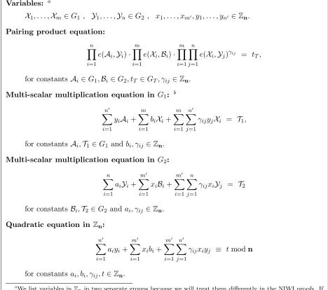
Variables: a
X1, . . . ,Xm∈G1 , Y1, . . . ,Yn∈G2 , x1, . . . , xm0, y1, . . . , yn0 ∈Zn.
Pairing product equation:
n
Y
i=1
e(Ai,Yi)· m
Y
i=1
e(Xi,Bi)· m Y i=1 n Y j=1
e(Xi,Yj)γij = tT,
for constants Ai∈G1,Bi∈G2, tT ∈GT, γij ∈Zn.
Multi-scalar multiplication equation in G1: b
n0
X
i=1
yiAi+ m
X
i=1 biXi+
m X i=1 n0 X j=1
γijyjXi = T1,
for constants Ai,T1 ∈G1 and bi, γij ∈Zn.
Multi-scalar multiplication equation in G2:
n
X
i=1
aiYi+ m0
X
i=1
xiBi+ m0 X i=1 n X j=1
γijxiYj = T2
for constants Bi,T2∈G2 and ai, γij ∈Zn.
Quadratic equation in Zn:
n0
X
i=1 aiyi+
m0
X
i=1 xibi+
m0 X i=1 n0 X j=1
γijxiyj ≡ tmodn
for constants ai, bi, γij, t∈Zn.
aWe list variables in
Zn in two separate groups because we will treat them differently in the NIWI proofs. If
we wish to deal with only one group of variables inZnwe can add equations inZn of the formx1=y1, x2=y2,
etc.
b
With multiplicative notation, these equations would be multi-exponentiation equations. We use additive notation forG1 andG2, since this will be notationally convenient in the paper, but again stress that the discrete
logarithm problem will typically be hard in these groups.
Figure 1: Equations over groups with bilinear map.
instantiations. The instantiations illustrate the variety of ways bilinear groups can be constructed. We can choose prime order groups or composite order groups, we can haveG1=G2 and G1 6=G2,
and we can make various cryptographic assumptions. All three security assumptions have been used in the cryptographic literature to build interesting protocols.
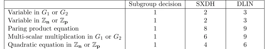
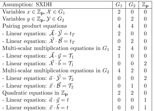
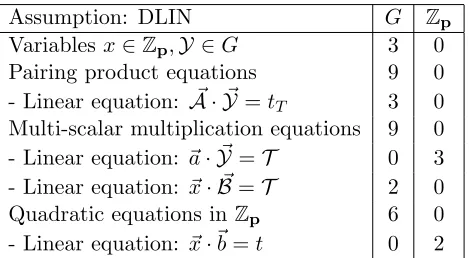
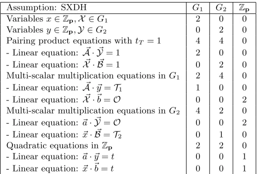
For all three instantiations, the techniques presented here yield efficient witness-indistinguishable proofs. In particular, the cost in proof size of each extra equation is constant and independent of the number of variables in the equation. The size of the proofs can be computed by adding the cost, measured in group elements fromG1 or G2, of each variable and each equation listed in Figure 1.
with care because the size of a group element depends on the type of bilinear group [GPS08]. We expect the SXDH-based instantiation to yield the smallest proofs when taking the sizes of group elements into account.
Subgroup decision SXDH DLIN
Variable in G1 orG2 1 2 3
Variable in Zn orZp 1 2 3
Paring product equation 1 8 9
Multi-scalar multiplication in G1 orG2 1 6 9
Quadratic equation inZn orZp 1 4 6
Table 1: Number of group elements each variable or equation adds to the size of a NIWI proof.
1.2 Related work
As we mentioned before, early work on NIZK proofs demonstrated that all NP-languages have non-interactive proofs, but did not yield efficient proofs. One cause for these proofs being inefficient in practice was the need for an expensive NP-reduction to, e.g., Circuit Satisfiability. Another cause of inefficiency was the reliance on the so-called hidden bits model, which even for small circuits is inefficient.
Groth, Ostrovsky, and Sahai [GOS06b, GOS06a] investigated NIZK proofs for Circuit Satisfia-bility using bilinear groups. This addressed the second cause of inefficiency since their techniques give efficient proofs for Circuit Satisfiability, but to use their proofs one must still make an NP-reduction to Circuit Satisfiability. We stress that while [GOS06b, GOS06a] used bilinear groups, their application was to build proof systems for Circuit Satisfiability. Here, we devise entirely new techniques to deal with general statements about equations in bilinear groups, without having to reduce to an NP-complete language.
Addressing the issue of avoiding an expensive NP-reduction, we have works by Boyen and Wa-ters [BW06, BW07] that suggest efficient NIWI proofs for statements related to group signatures. These proofs are based on bilinear groups of composite order and rely on the subgroup decision assumption.
Groth [Gro06] was the first to suggest a general group-dependent language and NIZK proofs for statements in this language. He investigated satisfiability of pairing product equations and only al-lowed group elements to be variables. He looked at the special case of prime order groupsG, GT with
a bilinear mape:G×G→GT and, based on the decisional linear assumption [BBS04], constructed
NIZK proofs for such pairing product equations. However, even for very small statements, the very different and much more complicated techniques of Groth yield proofs consisting of thousands of group elements (whereas ours would be in the tens). Our techniques are much easier to understand, significantly more general, and vastly more efficient.
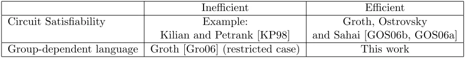
We summarize our comparison with other works on NIZK proofs in Table 2.
We note that there have been many earlier works (starting with [GMR89]) dealing with efficient
Inefficient Efficient
Circuit Satisfiability Example: Groth, Ostrovsky
Kilian and Petrank [KP98] and Sahai [GOS06b, GOS06a] Group-dependent language Groth [Gro06] (restricted case) This work
Table 2: Classification of NIZK proofs according to usefulness.
1.3 New techniques
[GOS06b, GOS06a, Gro06] start by constructing non-interactive proofs for simple statements and then combine many of them to get more powerful proofs. The main building block in [GOS06b], for instance, is a proof that a given commitment contains either 0 or 1, which has little expressive power on its own. Our approach is the opposite: we directly construct proofs for very expressive languages; as such, our techniques are very different from previous work.
The way we achieve our generality is by viewing the groups G1, G2, GT as modules over the
ring Zn. The ring Zn itself can also be viewed as a Zn-module. We therefore look at the more
general question of satisfiability of quadratic equations over Zn-modules A1, A2, AT with a bilinear
map, see Section 3 for details. Since many bilinear groups with various cryptographic assumptions and various mathematical properties can be viewed as modules we are not bound to any particular bilinear group or any particular assumption.
Given modules A1, A2, AT with a bilinear map, we construct new modules B1, B2, BT, also
equipped with a bilinear map, and we map the elements inA1, A2, AT into B1, B2, BT. The latter
modules will typically be larger thereby giving us room to hide the elements of A1, A2, AT. More
precisely, we devise commitment schemes that map variables from A1, A2 to the modules B1, B2.
The commitment schemes are homomorphic both with respect to the module operations and also with respect to the bilinear map.
Our techniques for constructing witness-indistinguishable proofs are fairly involved mathemati-cally, but we will try to present some high level intuition here. (We give more detailed intuition later in Section 6, where we present our main proof system). The main idea is the following: because our commitment schemes are homomorphic and we equip them with a bilinear map, we can take the equation that we are trying to prove, and just replace the variables in the equation with com-mitments to those variables. Of course, because the commitment schemes are hiding, the equations will no longer be valid. Intuitively, however, we can extract out the additional terms introduced by the randomness of the commitments: if we give away these terms in the proof, then this would be a convincing proof of the equation’s validity (again, because of the homomorphic properties). But, giving away these terms might destroy witness indistinguishability. Suppose, however, that there is only one “additional term” introduced by substituting the commitments. Then, because it would be the unique value which makes the equation true, giving it away would preserve witness indistinguishability! In general, we are not so lucky. But if there are many terms, the nice alge-braic environment allows us to randomize the terms such that their distribution is uniform over all possible terms satisfying the equation. We now get witness indistinguishability because all possible witnesses after randomization yield the same uniform distribution of terms satisfying the equation.
1.4 Applications
Subsequent to the announcement of our work, several papers have built upon it: Chandran, Groth and Sahai [CGS07] have constructed ring-signatures of sub-linear size using the NIWI proofs in the first instantiation, which is based on the subgroup decision problem. Groth and Lu [GL07] have used the NIWI and NIZK proofs from the third instantiation to construct a NIZK proof for the correctness of a shuffle. Groth [Gro07] has used the NIWI and NIZK proofs from the third in-stantiation to construct a fully anonymous group signature scheme. Belenkiy, Chase, Kohlweiss and Lysyanskaya [BCKL08] have used the second and third instantiations to construct non-interactive anonymous credentials. Green and Hohenberger [GH08] have used the third instantiation in a universally composable adaptive oblivious transfer protocol. Also, by attaching NIZK proofs to semantically secure public-key encryption in any instantiation, we get an efficient non-interactive verifiable cryptosystem. Boneh [Bon06] has suggested using this for optimistic fair exchange [Mic03], where two parties use a trusted but lazy third party to guarantee fairness.
1.5 Roadmap
The main result is the NIWI proof that can be found in Section 7. Sections 3, 4, 5 and 6 explain the structure of the NIWI proof, which goes through modules, commitments, a description of the com-mon reference string, and an explanation of how the NIWI proof works. For a concrete illustration of the steps, we refer the reader to the instantiation in Section 8. Other instantiations are given in Section 9 and Section 10. In many cases, our NIWI proofs can also be used as NIZK proofs, which we discuss in Section 11.
2
Non-interactive witness-indistinguishable proofs
Notation. We write y = A(x;r) when the algorithm A, on input x and randomness r, outputs
y. We write y ← A(x) for the process of picking randomness r uniformly at random and setting
y = A(x;r). More generally, we write y ← S for sampling y from the set S according to some probability distribution on S, using the uniform distribution as the default when nothing else is specified.
We write a←A;b← B(a);. . . for running the experiment wherea is chosen fromA, then b is chosen fromB, which may depend ona, etc. This yields a probability distribution over the outputs and we write Prha←A;b←B(a);. . .:C(a, b, . . .)ifor the probability of the condition C(a, b, . . .) being satisfied after running the experiment.
The security of our schemes is governed by a security parameterk, which can be used to scale up the security. Given two functionsf, g:N→[0,1] we writef(k)≈g(k) when|f(k)−g(k)|=O(k−c)
for every constant c. We say that f is negligible when f(k) ≈ 0 and that it isoverwhelming when
f(k)≈1. We say that two families of probability distributions{S1(k)}k∈N,{S2(k)}k∈Nare perfectly indistinguishable when they are the same for all sufficiently large k ∈ N, and we say they are computationally indistinguishable if for all non-uniform polynomial time adversariesA we have
Pr
h
y←S1(k) :A(1k, y) = 1
i
≈Pr
h
y←S2(k) :A(1k, y) = 1
i
.
Group dependent languages. LetR be an efficiently computable ternary relation. For triplets (gk, x, w) ∈ R we call gk the setup, x the statement and w the witness. Given some gk we let L
Non-interactive proofs. A non-interactive proof system for a relation R with setup consists of four probabilistic polynomial time algorithms: a setup algorithm G, a common reference string (CRS) generation algorithmK, a prover P and a verifier V. The setup algorithm outputs a setup (gk, sk). In our paper, gk will be a description of a bilinear group. The setup algorithm may output some related information sk, for instance the factorization of the group order. A cleaner case, however, is when sk is just the empty string, meaning the protocol is built on top of the group without knowledge of any trapdoors. The CRS generation algorithm takes (gk, sk) as input and produces a common reference stringσ. The prover takes as input (gk, σ, x, w) and produces a proof π. The verifier takes as input (gk, σ, x, π) and outputs 1 if the proof is acceptable and 0 if rejecting the proof. We call (G, K, P, V) a non-interactive proof system forR with setup G if it has the completeness and soundness properties described below.
Perfect completeness. A non-interactive proof is complete if an honest prover can convince an honest verifier whenever the statement belongs to the language and the prover holds a witness testifying to this fact.
Definition 1 (Perfect completeness) We say (G, K, P, V) is perfectly complete if for all adver-saries A we have2
Pr
h
(gk, sk)← G(1k);σ ←K(gk, sk); (x, w)← A(gk, σ);π←P(gk, σ, x, w) :
V(gk, σ, x, π) = 1 if (gk, x, w)∈Ri= 1.
Perfect soundness. A non-interactive proof is sound if it is impossible to prove a false statement.
Definition 2 (Perfect soundness) We say(G, K, P, V)is perfectly sound if for all adversaries A
we have
Prh(gk, sk)← G(1k);σ ←K(gk, sk); (x, π)← A(gk, σ) :V(gk, σ, x, π) = 0 if x /∈Li= 1.
Perfect culpable soundness. In the standard definition of soundness given above, the adversary tries to create a valid proof forx∈L¯. Groth, Ostrovsky and Sahai [GOS06b, Gro06] generalized the notion of soundness to disallowing false proofs of statements x ∈Lguilt, whereLguilt is a language
that may depend on gk and σ. They call this notion culpable soundness.3 Standard soundness is a special case with Lguilt = ¯L, but the notion can be used to capture other interesting cases as
well. The instantiation in Section 8 uses groups of composite order n=pq and offers an example where culpable soundness captures the inability of the adversary to produce convincing proofs for statements that are false in the orderp subgroups of Gand GT (here Lguilt⊆L¯ is the language of
statements that are false in the orderp subgroups).
Definition 3 (Perfect culpable soundness) We say (G, K, P, V) has perfect Lguilt-soundness if for all adversaries A we have
Prh(gk, sk)← G(1k);σ ←K(gk, sk); (x, π)← A(gk, σ) :V(gk, σ, x, π) = 0 if x∈Lguilt
i
= 1.
2Since the probability is exactly 1, the definition quantifies over allgk in the support ofG and all (gk, x, w)∈R. 3
Composable witness indistinguishability. A statement may have many possible witnesses. A non-interactive proof is witness indistinguishable if the proof does not reveal which of those witnesses the prover has used. The standard definition of witness-indstinguishability requires that proofs using different witnesses for the same statement are computationally indistinguishable. We will obtain a stronger definition of witness indistinguishability called composable witness indistinguishability. In this definition there is a reference string simulatorS that generates a simulated CRS and we require that the adversary cannot distinguish a real CRS from a simulated CRS. We also require that on a simulated CRS there is no information whatsoever to distinguish the different witnesses that might have been used to construct the proof. The advantage of this definition is that different types of proofs using the same type of real/simulated CRS can share the same CRS, which facilitates easier security proofs. We will use this composability property in the instantiations in Sections 8, 9 and 10.
Definition 4 (Composable witness indistinguishability) We say (G, K, P, V) is composable witness indistinguishable, if there is a probabilistic polynomial time simulator S, such that for all non-uniform polynomial time adversariesA we have
Prh(gk, sk)← G(1k);σ←K(gk, sk) :A(gk, σ) = 1i
≈ Pr
h
(gk, sk)← G(1k);σ←S(gk, sk) :A(gk, σ) = 1
i
,
and for all adversaries A we have
Pr
h
(gk, sk)← G(1k);σ←S(gk, sk); (x, w0, w1)← A(gk, σ);π ←P(gk, σ, x, w0) :A(π) = 1
i
= Prh(gk, sk)← G(1k);σ←S(gk, sk); (x, w0, w1)← A(gk, σ);π ←P(gk, σ, x, w1) :A(π) = 1
i
,
where we require (gk, x, w0),(gk, x, w1)∈R.
Composable zero-knowledge. A zero-knowledge proof, is a proof that shows the statement is true, but does not reveal anything else. Traditionally, this is defined by having a simulator (S1, S2) that can simulate the CRS and the proof, resepctively. The first part of the simulator
outputs a simulated CRS and a simulation trapdoorτ, and the second part of the simulator uses the simulation trapdoor to simulate proofs for statements without knowing the corresponding witnesses. The standard definition of (multi-theorem) zero-knowledge then says that real proofs on a real CRS should be computationally indistinguishable from simulated proofs on a simulated CRS.
We will obtain a strong notion of zero-knowledge, called composable zero-knowledge [Gro06]. Composable zero-knowledge implies standard zero-knowledge [Gro06] and has the advantage that it is simpler to work with, since it separates the computational indistinguishability into two separate parts addressing the CRS and the proofs, respectively. In composable zero-knowledge, the real CRS and the simulated CRS are computationally indistinguishable. Moreover, the adversary,even when it gets access to the secret simulation keyτ, cannot distinguish real proofs from simulated proofs on a simulated CRS.
Definition 5 (Composable zero-knowledge) We say(G, K, P, V)is composable zero-knowledge if there exists a probabilistic polynomial time simulator(S1, S2) such that for all non-uniform poly-nomial time adversaries A we have
Pr
h
(gk, sk)← G(1k);σ←K(gk, sk) :A(gk, σ) = 1
i
≈ Prh(gk, sk)← G(1k); (σ, τ)←S1(gk, sk) :A(gk, σ) = 1
i
and for all interactive adversariesA we have
Pr
h
(gk, sk)← G(1k); (σ, τ)←S1(gk, sk); (x, w)← A(gk, σ, τ);π ←P(gk, σ, x, w) :A(π) = 1
i
= Prh(gk, sk)← G(1k); (σ, τ)←S1(gk, sk); (x, w)← A(gk, σ, τ);π ←S2(gk, σ, τ, x) :A(π) = 1
i
,
where A outputs(x, w) so (gk, x, w)∈R.
3
Modules with bilinear maps
Let (R,+,·,0,1) be a finite commutative ring. Recall that an R-module A is an abelian group (A,+,0) where the ring acts on the group such that for allr, s∈ R and all x, y∈A
(r+s)x=rx+sx r(x+y) =rx+ry r(sx) = (rs)x 1x=x.
A cyclic group Gof order n can in a natural way be viewed as a Zn-module. We observe that
all the equations in Figure 1 can be viewed as equations overZn-modules with a bilinear map. To
generalize completely, let R be a finite commutative ring and let A1, A2, AT be finite R-modules
with a bilinear map f : A1 ×A2 → AT. We will consider quadratic equations over variables x1, . . . , xm∈A1, y1, . . . , yn∈A2 of the form
n
X
j=1
f(aj, yj) + m
X
i=1
f(xi, bi) + m
X
i=1 n
X
j=1
γijf(xi, yj) =t.
In order to simplify notation, let us for x1, . . . , xn∈A1, y1, . . . , yn∈A2 define
~ x·~y=
n
X
i=1
f(xi, yi).
The equations can now be written as
~a·~y+~x·~b+~x·Γ~y=t,
where~a∈An1,~b ∈A2m,Γ∈Matm×n(R). We note for future use that due to the bilinear properties
off, we have for any matrix Γ∈Matm×n(R) and for any~x∈Am1 , ~y∈An2 that~x·Γy~= Γ>~x·~y.
Let us now return to the equations in Figure 1 and see how they can be recast as quadratic equations overZn-modules with a bilinear map.
Pairing product equations: Define R=Zn, A1 =G1, A2 =G2, AT =GT, f(x, y) = e(x, y) and
rewrite4 the pairing product equation as (A ·~ Y~)(X ·~ B~)(X ·~ ΓY~) =tT.
Multi-scalar multiplication in G1: Define R =Zn, A1 =G1, A2 =Zn, AT =G1, f(X, y) = yX
and rewrite the multi-scalar multiplication equation asA ·~ ~y+X ·~ ~b+X ·~ Γ~y=T1.
Multi-scalar multiplication in G2: Define R =Zn, A1 =Zn, A2 =G2, AT = G2, f(x,Y) =xY
and rewrite the multi-scalar multiplication equation as~a·Y~ +~x·B~+~x·ΓY~ =T2.
Quadratic equation in Zn: Define R = Zn, A1 = Zn, A2 = Zn, AT = Zn, f(x, y) = xymodn
and rewrite the quadratic equation inZn as~a·~y+~x·~b+~x·Γ~y≡tmodn.
We will therefore first focus on the more general problem of constructing non-interactive composable witness-indistinguishable proofs for satisfiability of quadratic equations overR-modulesA1, A2, AT
(using additive notation for all modules) with a bilinear mapf :A1×A2→AT.
4
We use multiplicative notation here, because, usuallyGT is written multiplicatively in the literature. When we
4
Commitment from modules
In our NIWI and NIZK proofs we will commit to the variables x1, . . . , xm ∈ A1, y1, . . . , yn ∈ A2.
We do this by mapping them into other R-modules B1, B2 and making the commitments in those
modules.
Let us for now just consider how to commit to elements from one R-moduleA. The public key for the commitment scheme will describe anotherR-module B and R-linear maps ι:A → B and
p:B →A. Operations in the module and computation of the map ι will be efficiently computable butp is hard to compute.5 The public key will also contain elements u1, . . . , umˆ ∈ B. To commit
tox∈A we pickr1, . . . , rmˆ ← Rat random and compute the commitment
c:=ι(x) +
ˆ m
X
i=1 riui.
Our commitment scheme will have two types of commitment keys.
Binding key: A binding key defines (B, ι, p, u1, . . . , umˆ) where ∀i : p(ui) = 0 and p ◦ι is
non-trivial. The commitment c:=ι(x) +Pmˆ
i=1riui therefore contains the non-trivial information p(c) =p(ι(x)) aboutx. In particular, ifp◦ιis the identity map on A, then the commitment is perfectly binding tox.
Hiding key: A hiding key defines (B, ι, p, u1, . . . , umˆ) whereι(A)⊆ hu1, . . . , umˆi. The commitment c := ι(x) +Pmˆ
i=1riui therefore perfectly hides the element x when r1, . . . , rmˆ are chosen at
random fromR.
Computational indistinguishability: For security we need binding keys and hiding keys to be computationally indistinguishable. Witness-indistinguishability of our NIWI proofs and later the zero-knowledge property of our NIZK proofs will rely on this.
The treatment of commitments using the language of modules generalizes several previous works dealing with commitments over bilinear groups, including [BGN05, GOS06b, GOS06a, Gro06, Wat06].
Since we will often be committing to many elements at a time let us define some convenient notation. Given elements x1, . . . , xm ∈ A we will write~c := ι(x~) +R~u with R ∈ Matm×mˆ(R) for
making commitmentsc1, . . . , cm computed asci:=ι(xi) +Pmj=1ˆ rijuj.
5
Setup
In our NIWI and NIZK proofs the setup and the common reference string are
gk defining (R, A1, A2, AT, f),
σ together with gk defining (B1, B2, BT, F, ι1, p1, ι2, p2, ιT, pT, ~u, ~v, H1, . . . , Hη).
Part of the common reference string specifies B1, ι1, p1, u1, . . . , umˆ and B2, ι2, p2, v1, . . . , vˆn that
are commitment keys forA1andA2. We note that many of these components may be given implicitly
instead of being described explicitly in the common reference string.
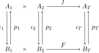
Another part of the common reference string specifies a third R-module BT together with R
A1 × A2 AT
B1 × B2 BT ι1 p1 ι2 p2 ιT pT
f
F
∀x∈A1 ∀y ∈A2 : F(ι1(x), ι2(y)) =ιT(f(x, y))
∀x∈B1 ∀y∈B2: f(p1(x), p2(y)) =pT(F(x, y))
Figure 2: Modules and maps between them.
that the maps are commutative as described in Figure 2 below, and with the exception ofp1, p2 and pT, that they are efficiently computable.
For notational convenience, we define for~x∈B1n, ~y∈B2n that
~ x•~y=
n
X
i=1
F(xi, yi).
Due to the bilinear properties ofF we have for all vectors and matrices with appropriate dimensions
~x•Γ~y= Γ>~x•~y.
The final part of the common reference string is a set of matricesH1, . . . , Hη ∈Matmˆ×nˆ(R) that
all satisfy ~u•Hi~v = 0. The exact number of matrices H1, . . . , Hη that is needed, depends on the
concrete setting. In many cases, we need no matrices at all and we haveη = 0, but there are also cases where they are needed as we shall see in the instantiation in Section 10.
There will be two different settings of interest to us.
Soundness setting: In the soundness setting, we have binding commitment keys. This means
p1(~u) =~0 and p2(~v) =~0, and the maps p1◦ι1 and p2◦ι2 are non-trivial. We will also want pT ◦ιT to be non-trivial.
Witness-indistinguishability setting: In the witness-indistinguishability setting we have hiding commitment keys, such thatι1(A1)⊆ hu1, . . . , umˆi andι2(A2)⊆ hv1, . . . , vnˆi. We also require
thatH1, . . . , Hη generate theR-module of all matricesH∈Matmˆ×ˆn(R) such that~u•H~v= 0.
As we will see in the next section, these matrices play a role in the randomization of the NIWI proofs.
Computational indistinguishability: The (only) computational assumption this paper is based on is that the two settings can be set up in a computationally indistinguishable way. The in-stantiations in Sections 8, 9 and 10 show that there are many ways to get such computationally indistinguishable soundness and witness-indistinguishability setups.
5
6
Proving that committed values satisfy a quadratic equation
Recall that in our setting, a quadratic equation looks like
~a·~y+~x·~b+~x·Γ~y=t, (1)
with constants~a∈An1,~b ∈Am2 ,Γ ∈Matm×n(R), t ∈AT. We will first consider the case of a single
quadratic equation of the above form. The first step in our NIWI proof will be to commit to all the variables~x, ~y. The commitments are of the form
~
c=ι1(~x) +R~u , d~=ι2(~y) +S~v, (2)
with R ∈ Matm×mˆ(R), S ∈ Matn׈n(R). The prover’s task is to convince the verifier that the
commitments contain ~x ∈ Am1 , ~y ∈ An2 that satisfy the quadratic equation. (Note that for all equations we will use these same commitments.)
Intuition. Before giving the construction let us give some intuition. In the previous sections, we have carefully set up our commitments such that the commitments themselves also “behave” like the values being committed to: they also belong to modules (theB modules) equipped with a bilinear map (the mapF, implicitly used in the •operation). Given that we have done this, a natural idea is to take the quadratic equation (1), and “plug in” the commitments (2) in place of the variables; let us evaluate
ι1(~a)•d~+~c•ι2(~b) +~c•Γd.~
After some computations, where we expand the commitments (2), make use of the bilinearity of•, and rearrange terms (the details can be found in the proof of Theorem 6) we get
ι1(~a)•ι2(~y) +ι1(~x)•ι2(~b) +ι1(~x)•Γι2(~y)
+ι1(~a)•S~v+R~u•ι2(~b) +ι1(x~)•ΓS~v+R~u•Γι2(~y) +R~u•ΓS~v.
By the commutative properties of the maps, the first group of three terms is equal to ιT(t), if (1)
holds. Looking at the remaining terms, note that~u and ~v are part of the common reference string and therefore known to the verifier. Using the fact that bilinearity implies that for any~x, ~y we have
~x•Γ~y= Γ>~x•~y, we can sort the remaining terms so they match either~u or~vto get (again see the proof of Theorem 6 for details)
ιT(t) +~u•
R>ι2(~b) +R>Γι2(~y) +R>ΓS~v
+S>ι1(~a) +S>Γ>ι1(~x)
•~v. (3)
Now, for the sake of intuition, let us make some simplifying assumptions. Let us assume that we are working in a symmetric case whereA1 =A2,B1 =B2,~u=~v, andF is symmetric, and so, the
above equation can be simplified further to get
ιT(t) +~u•
R>ι2(~b) +R>Γι2(~y) +R>ΓS~u+S>ι1(~a) +S>Γ>ι1(~x)
.
Now, suppose the prover gives to the verifier as his proof~π =R>ι2(~b) +R>Γι2(~y) +R>ΓS~u+
S>ι1(~a) +S>Γ>ι1(~x)
.The verifier would then check that the followingverification equation holds:
Suppose further p1◦ι1, p2◦ι2, pT ◦ιT are the identity maps onA1, A2, AT. It is easy to see that
the proof is convincing in the soundness setting, because in that setting we have that p1(~u) = ~0.
Then the verifier would know (but not be able to compute) that by applying the mapsp1, p2, pT we
get
~a•p2(d~) +p1(~c)•~b+p1(~c)•Γp2(d~) =t+p1(~u)•p2(~π) =t.
This gives us soundness, since~x:=p1(~c) and~y:=p2(d~) satisfy the equations.
The remaining problem is to get witness-indistinguishability. Recall that in the witness-indistinguishability setting, the commitments are perfectly hiding. Therefore, in the verification equation, nothing except for ~π holds any information about ~x and ~y (except for the information that can be inferred from the quadratic equation itself). So, let’s consider two cases:
1. Suppose that~πis the unique value such that the verification equation is valid. In this case, we trivially have witness indistinguishability, since the uniqueness means that any witness would lead to the same value for~π.
2. The simple case above might seem too good to be true, but let us see what it means if it is not true. If two proofs ~π and ~π0 both satisfy the verification equation, then subtracting the equations shows that ~u•(~π −~π0) = 0. On the other hand, recall that in the witness indistinguishability setting, the~u vectors generate the entire space where ~π and ~π0 live, and furthermore we know that the matricesH1, . . . , Hηgenerate allHsuch that~u•H~u= 0.
There-fore, let us chooser1, . . . , rη at random, and consider the distribution ~π00 =~π+Pηi=1riHi~u.
We obtain the same distribution on ~π00 that satisfies the verification equation regardless of whether we started from~π or~π0 or any other proof.
Thus, for the symmetric case we obtain a witness indistinguishable proof system. For the general non-symmetric case, instead of having just ~π for the ~u part of (3), we would also have a proof ~θ
for the ~v part. In this case, we would also have to make sure that this split does not reveal any information about the witness. What we will do is to randomize the proofs such that they get a uniform distribution on all ~π, ~θ that satisfy the verification equation. If we pick T ← Matˆn×mˆ(R)
at random we have that~θ+T ~ucompletely randomizesθ~. The part we add in~θcan be “subtracted” from~π by observing that
ιT(t) +~u•~π+θ~•~v=ιT(t) +~u•
~π−T>~v+~θ+T ~u•~v.
By randomizing~π this leads to a uniform distribution of proofs for the general non-symmetric case as well.
6.1 The general case
Having explained the intuition behind the proof system, we proceed to a formal description of how the prover handles a single equation and the security properties the procedure has.
Prover: Pick T ←Matˆn×mˆ(R), r1, . . . , rη ← Rat random. Compute
~
π := R>ι2(~b) +R>Γι2(~y) +R>ΓS~v−T>~v+ η
X
i=1 riHi~v
~
θ := S>ι1(~a) +S>Γ>ι1(~x) +T ~u
Verifier: Return 1 if and only if
ι1(~a)•d~+~c•ι2(~b) +~c•Γd~=ιT(t) +u~•~π+~θ•~v.
Perfect completeness of our NIWI proof will follow from the following theorem regardless of whether we are in the soundness setting or the witness-indistinguishability setting.
Theorem 6 Given ~x∈Am1 , ~y∈An2, R∈Matm×mˆ(R), S ∈Matn׈n(R) satisfying
~c=ι1(~x) +R~u d~=ι2(~y) +S~v ~a·~y+~x·~b+~x·Γ~y =t,
we have for all choices ofT, r1, . . . , rη that the proofs~π, ~θ constructed as above will be accepted.
Proof. The commutative property of the linear and bilinear maps gives us ι1(~a)•ι2(~y) +ι1(~x)• ι2(~b) +ι1(~x)•Γι2(~y) =ιT(t). For any choice of T, r1, . . . , rη we have
ι1(~a)•d~+~c•ι2(~b) +~c•Γd~
= ι1(~a)•
ι2(~y) +S~v
+ι1(~x) +R~u
•ι2(~b) +
ι1(~x) +R~u
•Γι2(~y) +S~v)
= ι1(~a)•ι2(~y) +ι1(~x)•ι2(~b) +ι1(~x)•Γι2(~y)
+R~u•ι2(~b) +R~u•Γι2(~y) +R~u•ΓS~v+ι1(~a)•S~v+ι1(~x)•ΓS~v
= ιT(t) +~u•
R>ι2(~b) +R>Γι2(~y) +R>ΓS~v
+S>ι1(~a) +S>Γ>ι1(~x)
•~v
= ιT(t) +~u•
R>ι2(~b) +R>Γι2(~y) +R>ΓS~v
+
η
X
i=1
ri(~u•Hi~v)−~u•T>~v
+T ~u•~v+S>ι1(~a) +S>Γ>ι1(~x)
•~v
= ιT(t) +~u•~π+θ~•~v
Theorem 7 In the soundness setting, where we havep1(~u) =~0 andp2(~v) =~0, a valid proof implies
p1(ι1(~a))·p2(d~) +p1(~c)·p2(ι2(~b)) +p1(~c)·Γp2(d~) =pT(ιT(t)).
Proof. An acceptable proof~π, ~θ satisfiesι(a)•d~+~c•ι2(~b) +~c•Γd~=ιT(t) +u~•~π+~θ•~v. The
commutative property of the linear and bilinear maps gives us
p1(ι1(~a))·p2(d~) +p1(~c)·p2(ι2(~b)) +p1(~c)·Γp2(d~)
= pT(ιT(t)) +p1(~u)·p2(~π) +p1(~θ)·p2(v~) =pT(ιT(t))
Observe as a particularly interesting case that whenp1◦ι1, p2◦ι2, pT ◦ιT are the identity maps
onA1, A2 andAT, respectively, this means~x:=p1(~c) and~y:=p2(d~) give us a satisfying solution to
the equation~a·~y+~x·~b+~x·Γ~y=t. In this case, the theorem says that the proof is perfectly sound in the soundness setting. In the case where they are not the identity maps it is still possible to have a form of culpable soundness, see the instantiation in Section 8 for an example based on composite order bilinear groups.
Theorem 8 In the witness-indistinguishable setting where ι1(A1) ⊆ hu1, . . . , umˆi, ι2(A2) ⊆
Proof. Since ι1(A1) ⊆ hu1, . . . , umˆi and ι2(A2) ⊆ hv1, . . . , vnˆi there exists A, B, X, Y such that ι1(~a) =A~u,ι1(~x) =X~uandι2(~b) =B~v, ι2(~y) =Y ~v. We have~c= (X+R)~uandd~= (Y +S)~v. The
proof is (~π, ~θ) given by
~
θ=S>ι1(~a) +S>Γ>ι1(~x) +T ~u=
S>A+S>Γ>X+T
~ u
~
π=R>ι2(~b) +R>Γι2(~y) +R>ΓS~v))−T>~v+ η
X
i=1 riHi~v
=
R>B+R>ΓY +R>ΓS−T>
~v+
Xη
i=1 riHi
~ v.
We chooseT at random, so we can think of ~θbeing a uniformly random variable given by ~θ= Θ~v
for a randomly chosen matrix Θ. We can think of~π as being written~π = Π~v, where Π is a random variable that depends on Θ.
By perfect completeness all satisfying witnesses yield proofs whereι1(~a)•d~+~c•ι2(~b) +~c•Γd~− ιT(t)−~θ•~v =~u•~π =~u•Π~v. Conditioned on the random variable Θ we therefore have that any
two possible solutions ~π, ~π0 satisfy ~u•(Π−Π0)~v = 0. Since H1, . . . , Hη generate all matrices H
such that ~u•H~v = 0 we can write this as Π = Π0+Pη
i=1r0iHi. In constructing~π we form it as
R>B+R>ΓY +R>ΓS−T>
~ v+
Pη
i=1riHi
~
v for randomly chosenr1, . . . , rη ∈ R. We therefore
get a uniform distribution over all~π that satisfy the equation conditioned on~θ. Since~θis uniformly chosen, we conclude that for any witness we get a uniform distribution over (~θ, ~π) conditioned on it
being an acceptable proof.
6.2 Linear equations
As a special case, we will consider the proof system when~a= 0 and Γ = 0. In this case the equation is simply
~
x·~b=t.
The scheme can be simplified in this case by choosing T = 0 in the proof, which gives ~θ:=~0 and
~π := R>ι2(~b) +Pηi=1riHi~v. Theorem 6 still applies with T = 0, which will give us completeness.
Theorem 7 says p1(~c)·p2(ι2(~b)) = pT(ιT(t)), which will give us soundness. Finally, we have the
following theorem.
Theorem 9 In the witness-indistinguishable setting where ι1(A1) ⊆ hu1, . . . , umˆi, ι2(A2) ⊆
hv1, . . . , vnˆi and H1, . . . , Hη generate all matrices H such that ~u•H~v = 0, all satisfying witnesses ~x, ~y, R, S yield the uniform distribution of the proof~π ∈ hv1, . . . , vnˆimˆ conditioned on the verification equation~c•ι2(~b) =ιT(t) +~u•~π being satisfied.
Proof. As in the proof of Theorem 8 we can write~π= Π~v. Any witness gives a proof that satisfies
~c•ι1(~b)−ιT(t) =~u•~π=~u•Π~v.
Since H1, . . . , Hη generate all matrices H such that ~u•H~v = 0 we have that Π has a uniform
distribution over all matrices Π satisfying the verification equation.
6.3 The symmetric case
An interesting special case is when B := B1 = B2, ˆm ≥ nˆ with u1 = v1, . . . , uˆn = vnˆ, and F is
symmetric case, we can simplify the scheme by just padding~θ with zeroes in the end to extend the length to ˆm, call this vector~θ0, and reveal the proofφ~ =~π+~θ0. In the verification, we check that
ι1(~a)•d~+~c•ι2(~b) +~c•Γd~=ιT(t) +~u•φ.~
Theorem 6 gives us completeness, and Theorem 8 implies that all witnesses yield the same distru-butions on the proofs ~π, ~θ and therefore the same distributions on the proofs φ~. With respect to soundness we have the following theorem.
Theorem 10 In the soundness setting, where we havep1(~u) =~0 a valid proof implies
p1(ι1(a))·p2(d~) +p1(~c)·p2(ι2(~b)) +p1(~c)·Γp2(d~) =pT(ιT(t)).
Proof. An acceptable proofφ~ satisfiesι1(~a)•d~+~c•ι2(~b) +~c•Γd~=ιT(t) +~u•~φ.The commutative
property of the linear and bilinear maps gives us
p1(ι1(~a))·p2(d~) +p1(~c)·p2(ι2(~b)) +p1(~c)·Γp2(d~) =pT(ιT(t)) +p1(~u)·p2(φ~) =pT(ιT(t)).
We can simplify the computation of the proof in the symmetric case. We have
~
π := R>ι2(~b) +R>Γι2(~y) +R>ΓS~v−T>~v+ η
X
i=1 riHi~v
~
θ := S>ι1(~a) +S>Γ>ι1(~x) +T ~u,
and extend θ to θ0 by padding it with ˆm−nˆ 0’s. Another way to accomplish this padding is by paddingT with ˆm−nˆ 0-rows andS with ˆm−nˆ 0-columns and eachHi with ˆm−nˆ 0-columns. We
then have
~
φ:=R>ι2(~b) +R>Γι2(~y) +R>ΓS0~u−(T0)>~u+ η
X
i=1
riHi0~u+ (S0)>ι1(~a) + (S0)>Γ>ι1(~x) +T0~u.
Since the map is symmetric we have~u•(T0−(T0)>)~u= 0. If we have a setH10, . . . , Hη00 that generates all matricesH0 such that~u•H0u~ = 0, then we have T0−(T0)> is in the span of them. This means the following simpler proof is also witness-indistinguishable
~
φ:=R>ι2(~b) +R>Γι2(~y) + (S0)>ι1(~a) + (S0)>Γ>ι1(~x) +R>ΓS0~u+ η0
X
i=1 riHi0~u.
7
NIWI proof for satisfiability of a set of quadratic equations
We will now give the full composable NIWI proof for satisfiability of a set of quadratic equations in a module with a bilinear map, i.e., the language
L=
n
{(~ai,~bi,Γi, ti)}Ni=1
∃~x, ~y ∀i:~ai·~y+x~·~bi+~x·Γi~y=ti o
.
The proof will haveLguilt-soundness for
Lguilt =
n
{(~ai,~bi,Γi, ti)}Ni=1
∀~x, ~y ∃i:p1(ι1(~ai))·~y+~x·p2(ι2(~bi)) +~x·Γi~y6=pT(ιT(ti)) o
Observe as an important special case that ifp1◦ι1, p2◦ι2, pT ◦ιT are the identity maps on A1, A2
andAT, thenLguilt = ¯L making soundness andLguilt-soundness the same notion.
The cryptographic assumption we make is that the common reference string is created by one of two algorithm K or S and that their outputs are computationally indistinguishable. The first algorithm outputs a common reference string that specifies a soundness setting, whereas the second algorithm outputs a common reference string that specifies a witness-indistinguishability setting.
Setup: (gk, sk) = ((R, A1, A2, AT, f), sk)← G(1k).
CRS generators: The common reference string defines (B1, B2, BT, F, ι1, p1, ι2, p2, ιT, pT, ~u, ~v, H1, . . . , Hη).
It can be generated as a soundness stringσ ← K(gk, sk) or as a witness-indistinguishability stringσ ←S(gk, sk).
Prover: The input consists ofgk, σ, a list of quadratic equations{(~ai,~bi,Γi, ti)}Ni=1and a satisfying
witness~x∈Am1 , ~y∈An2.
Pick at random R ← Matm×mˆ(R) and S ← Matn×nˆ(R) and commit to all the variables as ~c:=~x+R~u and d~:=~y+S~v.
For each equation (~ai,~bi,Γi, ti) make a proof as described in Section 6. In other words, pick Ti ←Matnˆ×mˆ(R) and ri1, . . . , riη ← Rand compute
~
πi := R>ι2(~bi) +R>Γiι2(~y) +R>ΓiS~v−Ti>~v+ η
X
j=1 rijHj~v
~
θi := S>ι1(~ai) +S>Γ>i ι1(~x) +Ti~u.
Output the proof (~c, ~d,{(~πi, ~θi)}Ni=1).
Verifier: The input is gk, σ,{(~ai,~bi,Γi, ti)}i=1N and the proof is (~c, ~d,{(~πi, ~θi)}Ni=1).
For each equation check
ι1(~ai)•d~+~c•ι2(~bi) +~c•Γid~=ιT(ti) +~u•~πi+~θi•~v.
Output 1 if all the checks pass, else output 0.
Theorem 11 The proof system (G, K, P, V) given above is a NIWI proof for satisfiability of a set of quadratic equations with perfect completeness, perfect Lguilt-soundness and composable witness-indistinguishability.
Proof. Perfect completeness follows from Theorem 6.
Consider a proof (~c, ~d,{(~πi, ~θi)}) on a soundness string. Definex~ :=p1(~c), ~y:=p2(d~). It follows
from Theorem 7 that for each equation we have
p1(ι1(~ai))·~y+~x·p2(ι2(~bi)) +~x·Γi~y
= p1(ι1(~ai))·p2(d~) +p1(~c)·p2(ι2(~bi)) +p1(~c)·Γip2(d~) =pT(ιT(ti)).
This means we have perfect Lguilt-soundness.
We have assumed that soundness strings and witness-indistinguishability strings are computa-tionally indistinguishable. Consider now a witness-indistinguishability stringσ. The commitments are perfectly hiding, so they do not reveal the witness~x, ~y that the prover uses in the commitments
~c, ~d. Theorem 8 says that in each equation either of two possible witnesses yields the same distri-bution on the proof for that equation. A straightforward hybrid argument then shows that we have
Proof of knowledge. We observe that if K outputs an additional secret piece of information
ξ that makes it possible to efficiently compute p1 and p2, then ξ makes it possible to extract the
witness~x=p1(~c) and ~y=p2(d~).
Proof size. The size of the common reference string is ˆm elements in B1 and ˆn elements in B2
in addition to the description of the modules, the maps and H1, . . . , Hη. The size of the proof is m+Nnˆ elements inB1 and n+Nmˆ elements inB2.
Typically, ˆm and ˆn will be small, giving us a proof size that is O(m+n+N) elements in B1
andB2. The proof size may thus be smaller than the description of the statement, which can be of
size up toN n elements inA1,N m elements inA2,N mn elements inRand N elements inAT.
7.1 NIWI proofs for bilinear groups
We will now outline the strategy for making NIWI proofs for satisfiability of a set of quadratic equations over bilinear groups. As we described in Section 3, there are four different types of equations corresponding to the following four combinations ofZn-modules:
Pairing product equations: A1 =G1, A2=G2, AT =GT, f(X,Y) =e(X,Y).
Multi-scalar multiplication in G1: A1 =G1, A2 =Zn, AT =G1, f(X, y) =yX.
Multi-scalar multiplication in G2: A1 =Zn, A2=G2, AT =G2, f(x,Y) =xY.
Quadratic equations in Zn: A1=Zn, A2 =Zn, AT =Zn, f(x, y) =xy modn.
The common reference string will specify commitment schemes to respectively scalars and group elements. We first commit to all the variables and then make the NIWI proofs that correspond to the types of equations that we are looking at. It is important that we use the same commitment schemes and commitments for all equations, i.e., for instance we only commit to a scalarxonce and we use the same commitment in the proof whetherxis involved in is a multi-scalar multiplication in
G2or a quadratic equations inZn. The use of the same commitment in all the equations is necessary
to ensure a consistent choice ofx throughout the proof. As a consequence of this we use the same moduleB10 to commit tox in both multi-scalar multiplication inG2 and quadratic equations inZn.
We therefore end up with at most four different modulesB1, B10, B2, B20 to commit to respectively
X, x,Y, y variables.
8
Instantiation based on the subgroup decision assumption
Setup. The first instantiation is based on the composite order groups introduced by Boneh, Goh and Nissim [BGN05]. The setup algorithm GBGN outputs (gk, sk) where gk = (n, G, GT, e,P)
describes a bilinear group of composite order n and sk = (p,q) consists of two primes such that
n = pq. Boneh, Goh and Nissim also introduced the subgroup decision assumption, which says that it is hard to distinguish a random element of orderqfrom a random element of ordern.
Definition 12 (Subgroup decision assumption) We say the subgroup decision assumption
holds for GBGN if for all non-uniform polynomial time A:
Pr[(gk, sk)← GBGN(1k);α ←Zn∗;U :=αpP :A(gk,U) = 1]
Statements. Based on the subgroup decision assumption we will construct NIWI proofs for the language consisting of pairing product equations, multi-scalar multiplication equations and quadratic equations as described in Figure 1. A statement consists of NP pairing product equations of the
form Q
ie(Ai,Yi) ·
Q
i,je(Yi,Yj)γij = tT, NM multi-scalar multiplication equations of the form
P
iaiYi+
P
ixiBi+
P
i,jγijxiYj =T andNQquadratic equations of the form
P
iaixi+
P
i,jγijxixj ≡ tmodn, and a claim that there are x1, . . . , xm ∈Zn andY1, . . . ,Yn∈G that satisfy all equations.
Formally, given a setupgk= (n, G, GT, e,P) we define the language:
L = n{(A~i,ΓPi , tT i)}Ni=1P,{(~ai, ~Bi,ΓMi ,Ti)}Ni=1M,{(~bi,ΓQi , ti)} NQ
i=1 ∃m, n∈N∃~x∈Z
m
n∃Y ∈~ Gn:
∀i∈[NP] :A~i ∈Gn ∧ ΓPi ∈Matn×n(Zn) ∧tT i ∈GT ∧ (A~i·Y~)(Y ·~ ΓPiY~) =tT i
∧ ∀i∈[NM] :~ai ∈Zmn ∧B~i ∈Gn∧ΓMi ∈Matm×n(Zn)∧ Ti∈G∧~ai·Y~+~x·B~i+~x·ΓMi Y~ =Ti
∧ ∀i∈[NQ] :~bi∈Zmn ∧ Γ Q
i ∈Matm×m(Zn) ∧ ti∈Zn∧ x~·~bi+~x·ΓPi~x≡ti modn
o
.
Soundness will hold in the orderpsubgroups of G, GT and Zn. More precisely, defineλ∈Zn as an
integer satisfyingλ≡1 modp and λ≡0 modq. Then λZn is the orderp subgroup of Zn and λG
is the orderp subgroup of G. We will getLguilt-soundness for
Lguilt =
n
{(A~i,ΓiP, tT i)}Ni=1P,{(~ai, ~Bi,ΓMi ,Ti)}N
M
i=1,{(~bi,ΓQi , ti)}i=1NP ∀m, n∈N∀~x∈(λZn)
m∀Y ∈~ (λG)n:
∃i∈[NP] :A~i ∈/Gn ∨ ΓPi ∈/Matn×n(Zn) ∨tT i∈/ GT ∨ (A~i·Y~)(Y ·~ ΓPi Y~)6=tTλi
∨ ∃i∈[NM] :~ai∈/ Zmn ∨B~i∈/ Gn∨ΓMi ∈/ Matm×n(Zn)∨ Ti ∈/ G∨~ai·Y~ +~x·B~i+~x·ΓMi Y 6~ =λTi
∨ ∃i∈[NQ] :~bi ∈/Zmn ∨ Γ Q
i ∈/Matm×m(Zn) ∨ ti ∈/Zn∨ ~x·~bi+~x·Γ Q
i ~x6≡ti modp
o
.
Multi-scalar multiplication equations. We will build our full NIWI proof from a combination of NIWI proofs for pairing-product equations, multi-scalar multiplication equations and quadratic equations. First consider the case where we only have multi-scalar multiplication equations. Define
LM (LMguilt) to be L (Lguilt) restricted to NP = NQ = 0 such that it only has NM multi-scalar
multiplication equations.
We can use our framework to get NIWI proofs for LM. The multi-scalar multiplication case corresponds to R = Zn, A1 = Zn, A2 = G, AT = G, f(x,Y) = xY and equations of the form ~a·Y~ +~x·B~+~x·ΓY~ =T over variables ~x∈Am1 and Y ∈~ An2.
The setup gk = (n, G, GT, e,P) implicitly defines A1, A2, AT, f. It also implicitly defines B1 = B2 =BT =Gand F(X,Y) =e(X,Y) and the linear maps6
ι1(x) =xP ι2(Y) =Y ιT(T) =e(P,T) p1(xP) =λxmodn p2(Y) =λY pT(e(P,T)) =λT.
Sinceλ2 ≡λmodn the maps commute as described in Figure 2. That is, we have
(x,Y) xY
(xP,Y) e(P, xY) (ι1, ι2) ιT
f
F
6
and we have
(λx, λY) λxY
(xP,Y) e(P, xY)
(p1, p2) pT
f
F
The common reference string σ consists of an element U ∈ G. In the soundness setting it is generated as U = αpP and in the witness-indistinguishability setting it is generated as U = αP, where α ← Z∗
n. The subgroup decision assumption implies that soundness strings and
witness-indistinguishability strings are computationally indistinguishable.
We will be usingU as a commitment key in bothB1and inB2. In order to commit tox∈A1 =Zn
we pickr ∈Zn and compute the commitmentC := ι1(x) +rU =xP +rU ∈B1 = G. In order to
commit toY ∈A2=Gwe picks←Zn and compute the commitmentD:=ι2(Y) +sU =Y+sU ∈ B2 =G.
On a soundness string, U describes a binding key for both commitment schemes. We have
p1(U) ≡p1(αpP)≡λαP ≡0 modn and p2(U) =λαpU =O. Furthermore, the maps p1◦ι1(x) = p1(xP) =λxmodn and p2◦ι2(Y) =p2(Y) =λY and pT ◦ιT(T) =pT(e(P,T)) =λT are all
non-trivial. A commitment C ∈ B1 defines the committed value uniquely in λZn, and a commitment
D ∈B2 defines the committed value uniquely inλG.
On a witness-indistinguishability string,U describes a hiding key for both commitment schemes. Since U is a generator forB1 =B2=Gwe have ι1(A1) =ι1(Zn) =G=hU i and ι2(A2) =ι2(G) = G = hU i. This implies that the commitment schemes are perfectly hiding. The only solution
H∈Mat1×1(Zn) toU •HU = 1, i.e., e(U, HU) = 1 is H = 0. We do therefore not need to include
any H1, . . . , Hη in the common reference string.
Theorem 11 now gives us a NIWI proof for the simultaneous satisfiability of a set of multi-scalar multiplication equations with perfect completeness, perfectLMguilt-soundness and composable witness-indistinguishability.
Pairing product equations. Now consider the case where we only have pairing product equa-tions. Define LP (LPguilt) to be L (Lguilt) restricted to NM = NQ = 0 such that it only has NP
pairing product equations. Using our framework, this corresponds to R=Zn, A1 =A2 =G, AT = GT, f(x, y) =e(x, y), and equations of the form (A ·~ Y~)(Y ·~ ΓY~) =tT over variables Y1, . . . ,Yn∈G.
The setup also defines modulesB1=B2 =GandBT =GT and the bilinear mapF(X,Y) =e(X,Y).
We use the mapsι2(Y) =Y and p2(Y) =λY described in the multi-scalar multiplication case above
together with ιT(zT) =zT and pT(zT) =zTλ to get the commutative diagram
A1 =G × A2=G AT =GT
B1 =G × B2=G BT =GT ι2 p2 ι2 p2 ιT pT
f(X,Y) =e(X,Y)
Using the same type of common reference string as in the multi-scalar multiplication case de-scribed above, we get a NIWI proof for the simultaneous satisfiability of pairing product equations with perfect completeness, perfectLPguilt-soundness and composable witness-indistinguishability.
Quadratic equations in Zn. Finally, consider the case where we only have quadratic equations.
Define LQ (LQguilt) to be L (Lguilt) restricted to NP =NM = 0 such that it only hasNQ quadratic
equations inZn. Using our framework, this corresponds toR=Zn, A1 =A2 =AT =Zn, f(x, y) = xymodn, and equations of the form~x·~b+~x·Γ~x≡tmodnover variablesx1, . . . , xm ∈Zn. The setup
also defines modulesB1=B2 =GandBT =GT and the bilinear mapF(xP, yP) =e(xP, yP). We
use the mapsι1(x) =xP and p1(xP) =λx described in the multi-scalar multiplication case above
together with ιT(t) =e(P, tP) and pT(e(P, tP)) =λtmodnto get the commutative diagram
A1 =Zn × A2 =Zn AT =Zn
B1=G × B2 =G BT =GT ι1 p1 ι1 p1 ιT pT
f(x, y) =xymodn
F(X,Y) =e(X,Y)
Using the same type of common reference string as in the multi-scalar multiplication case de-scribed above, we get a NIWI proof for the simultaneous satisfiability of quadratic equations with perfect completeness, perfectLQguilt-soundness and composable witness-indistinguishability.
The general case. In the three special cases described above, we used the same type of common reference string σ = U. To get a NIWI proof for the simultaneous satisfiability of equations we will combine them by using the sameU for all three types of equations. The same commitments to scalarsxi∈Zn are used in both multi-scalar multiplication equations and in quadratic equations in
Zn and the same commitments to variablesYj ∈Gare used in both pairing product equations and
in multi-scalar multiplication equations to enforce consistency accross different types of equations. The full NIWI proof forL is as follows:
Setup: (gk, sk) := ((n, G, GT, e,P),(p,q))← G(1k), where n=pq.
Soundness string: On input (gk, sk) return σ:=U where U :=rpP for randomr ∈Z∗n.
Witness-indistinguishability string: On input (gk, sk) returnσ:=U whereU :=rP for random
r∈Z∗ n.
Prover: On input (n, G, GT, e,P,U), a set of N =NP+NM+NQ equations, and a witness ~x, ~Y
do:
1. Commit to the scalarsx1, . . . , xm∈Zn and the group elementsY1, . . . ,Yn∈Gas
Ci :=xiP+riU Di :=Yi+siU
for randomly chosen~r ∈Zm
n, ~s∈Znn.
2. For each pairing product equation (A ·~ Y~)(Y ·~ ΓY~) = tT make a proof as described in
Section 6.3
φ := ~s>A~+~s>(Γ + Γ>)Y~ +~s>Γ~sU
=
n
X
i=1
siAi+ n
X
i=1 n
X
j=1
(γij +γji)siYj+ n
X
i=1 n
X
j=1
3. For each multi-scalar multiplication equation~a·Y~ +~x·B~+~x·ΓY~ =T the proof is
φ: = ~r>B~+~r>ΓY~+~r>Γ~sU+~s>~aP+~s>Γ~xP
=
m
X
i=1 riBi+
m X i=1 n X j=1
riγijYj+ m X i=1 n X j=1
γijrisjU + n
X
i=1
si(ai+ m
X
j=1
γijxj)P.
4. For each quadratic equation~x·~b+~x·Γ~x=tinZn we have
φ := ~r>~bP+~r>(Γ + Γ>)~xP+~r>Γ~rU
= (
m
X
i=1 ribi+
m X i=1 m X j=1
(γij +γji)rixj)P+ m X i=1 m X j=1
γijrirjU.
Verifier: On input (n, G, GT, e,P,U), a set of equations and a proof C~, ~D,{φi}Ni=1 do:
1. For each pairing product equation (A ·~ Y~)(Y ·~ ΓY~) =tT with proofφcheck that
n
Y
i=1
e(Ai,Di)· n Y i=1 n Y j=1
e(Di,Dj)γij =tTe(U, φ).
2. For each multi-scalar multiplication~a·Y~ +~x·B~+~x·ΓY~ =T with proofφcheck that
n
Y
i=1
e(aiP,Di)· m
Y
i=1
e(Ci,Bi)·
m Y i=1 n Y j=1
e(Ci,Dj)γij =e(P,T)e(U, φ).
3. For each quadratic equation~x·~b+~x·Γ~x=tinZn with proofφ check that
m
Y
i=1
e(Ci, biP)· m Y i=1 m Y j=1
e(Ci,Cj)γij =e(P,P)te(U, φ).
Theorem 13 The NIWI proof for Lgiven above has perfect completeness, perfect Lguilt-soundness and composable witness-indistinguishability.
Proof. Perfect completeness follows from the perfect completeness of each of the three types of proofs. Perfect Lguilt-soundness follows from Theorem 10 since we use the same commitments and maps p1, p2 accross different types of equations thus making the orderp solutions ~x =p1(C~), ~Y =p2(D~)
consistent with each other for all three types of equations. The subgroup decision assumption implies that soundness and witness-indistinguishability common reference strings are indistinguishable. On a indistinguishability string the commitments are perfectly hiding and we get perfect
witness-indistinguishability from Theorem 8.
Size. The size of the NIWI proof is m+n+N group elements in G, where m is the number of variables in ~x, n is the number of variables in Y~ and N =NP+NM+NQ is the total number of
9
Instantiation based on the SXDH assumption
Setup. The setup algorithm GSXDH returns a prime order bilinear group gk = (p, G1, G2, GT, e,P1,P2). We will assume the decision Diffie-Hellman problem is hard in both groups,
i.e., the Symmetric External Diffie-Hellman (SXDH) assumption.
Definition 14 (SXDH assumption) We say the SXDH assumption holds for GSXDH if for all non-uniform polynomial timeA and all b∈ {1,2} we have
Pr[gk← GSXDH(1k);α, t←Z∗p :A(gk, αPb, tPb, αtPb) = 1]
≈ Pr[gk← GSXDH(1k);α, t, r ←Z∗p:A(gk, αPb, tPb, rPb) = 1]
Statements. The setup gk = (p, G1, G2, GT, e,P1,P2) defines the ring Zp and modules
Zp, G1, G2, GT and bilinear maps corresponding to multiplication in Zp, scalar multiplication in G1 and G2, and the pairinge:G1×G2 →GT.
With this setup we can define pairing product equations, multi-scalar multiplication equations and quadratic equations as follows:
Pairing product equations: Using our framework, this corresponds to R =Zp, A1 = G1, A2 = G2, AT =GT, f(x, y) =e(x, y), and equations of the form (A ·~ Y~)(X ·~ B~)(X ·~ ΓY~) =tT.
Multi-scalar multiplication in G1: Using our framework, this corresponds to R = Zp, A1 = G1, A2 =Zp, AT =G1, f(X, y) =yX, and equations of the form A ·~ ~y+X ·~ ~b+X ·~ Γ~y =T1.
Multi-scalar multiplication in G2: Using our framework, this corresponds to R = Zp, A1 =
Zp, A2 =G2, AT =G2, f(x,Y) =xY, and equations of the form~a·Y~ +~x·B~+~x·ΓY~ =T2.
Quadratic equation in Zp: Using our framework, this corresponds to R = Zp, A1 = Zp, A2 =
Zp, AT =Zp, f(x, y) =xy modp, and equations of the form~a·~y+~x·~b+~x·Γ~y =t.
We consider statements that consist of sets of pairing product equations, multi-scalar multipli-cations inG1 andG2, and quadratic equations as described above. The equations are over variables x1, . . . , xm0, y1, . . . , yn0 ∈ Zp and X1, . . . ,Xm ∈G1 and Y1, . . . ,Yn∈ G2. We let L be the language of statements where there exists a solution ~x, ~y, ~X, ~Y that simultaneously satisfies all equations of all types.
Commitments. Consider a group G of prime order p. With entry-wise addition we get the
Zp-module B:=G2. We will use a commitment key of the form
u1 = (P,Q) := (P, αP) u2 = (U,V),
where α ← Z∗p is chosen at random. We can choose u2 = (U,V) in two different ways: u2 := tu1
or u2 := tu1 −(O,P) for a random t ∈ Z∗p. The former choice of u2 gives a perfectly binding
commitment key, whereas the latter choice ofu2 gives a perfectly hiding commitment key. The two
types of commitment keys are computationally indistinguishable under the DDH assumption. Let us now describe how to commit to an elementX ∈G1 using randomnessr1, r2 ∈Zp:
ι(Z) := (O,Z) p(Z1,Z2) :=Z2−αZ1 c:=ι(X) +r1u1+r2u2.
On a binding key whereu2=tu1 we have thatp◦ιis the identity map onGandp(u1) =p(u2) =O.
On a hiding key on the other hand,u1 and u2 are linearly independent. This means u1, u2 form a
basis forB =G2 and ι(G)⊆ hu1, u2i giving a perfectly hiding commitment.
Commitment to a scalar x∈Zp using randomnessr ∈Zp works as follows:
u:=u2+ (O,P) ι0(z) :=zu p0(z1P, z2P) :=z2−αz1 c:=ι0(x) +ru1.
On a binding key p0◦ι0 is the identity map and p0(u1) = 0, so the commitment scheme is perfectly
binding, and in fact the commitment c = ((r +xt)P,(r+xt)Q+xP) is an ElGamal encryption of xP. On a hiding key we have u = tu1 so u ∈ hu1i, which implies ι0(Zp) ⊆ hu1i. A hiding key
therefore gives us a perfectly hiding commitment scheme.
Common reference string. The common reference string is of the form (u1, u2, v1, v2), where
(u1, u2) is a commitment key for the group G1 implicitly defining maps ι1, p1, ι01, p01 as described
above, and (v1, v2) is a commitment key for G2 implicitly defining maps ι2, p2, ι02, p02 as described
above.
We will always use B1 =G21, B2 =G22 and we defineBT :=G4T with addition being entry-wise
multiplication. The mapF is defined as follows:
F :G21×G22 →G4T (
X1 X2
,
Y1 Y2
)7→
e(X1,Y1) e(X1,Y2)
e(X2,Y1) e(X2,Y2)
.
On a witness-indistinguishability string, we have hiding commitment keys u1, u2
and v1, v2 where each pair of vectors is linearly independent. The four elements F(u1, v1), F(u1, v2), F(u2, v1), F(u2, v2) are also linearly independent in the
witness-indistinguishability scenario. This implies that ~u • H~v = 0 only has the trivial solution whereH is the 2×2 matrix with 0-entries. Therefore, the common reference string does not need to include any matricesH1, . . . , Hη for the pairing product equations. The same holds true for the
other types of equations, we do not need any matricesH1, . . . , Hη in the common reference string.
Pairing product equations. Consider first the restricted languageLP⊂L, where the statements only have pairing product equations. The common reference string describesR=Zp, A1 =G1, A2 = G2, AT = GT, and B1 = G21, B2 = G22, BT = G4T, and commitment keys u1, u2, v1, v2, and the
following commuting linear and bilinear maps:
(X,Y) e(X,Y)
O X
,
O Y
1 1
1 e(X,Y)
(ι1, ι2) ιT
f
F