Automatic Search of Differential Path in MD4
Pierre-Alain Fouque, Gaëtan Leurent, Phong Nguyen
Laboratoire d’Informatique de l’École Normale Supérieure, Département d’Informatique,
45 rue d’Ulm, 75230 Paris Cedex 05, France
{Pierre-Alain.Fouque,Gaetan.Leurent,Phong.Nguyen}@ens.fr
Abstract. In 2004, Wang et al. obtained breakthrough collision attacks on the main hash functions from the MD4 family. The attacks are differential attacks in which one closely follows the inner steps of the underlying compression function, based on a so-called
differential path. It is generally assumed that such differential paths were found “by hand”. In this paper, we present an algorithm which automatically finds suitable differential paths, in the case of MD4. As a first application, we obtain new differential paths for MD4, which improve upon previously known MD4 differential paths. This algorithm could be used to find new differential paths, and to build new attacks against MD4.
Key words: MD4, collisions, differential path.
1 Introduction
Hash functions are fundamental primitives used in many cryptographic schemes and protocols. In a breakthrough work, Wang et al. recently discovered devastating collision attacks [19,21,22,20] on the main hash functions from the MD4 family, e.g. MD4 [19], RIPE-MD [19], MD5 [21], SHA-0 [22] and SHA-1 [20]. Such attacks can find collisions in much less time than the birthday paradox. Despite the efficiency of these new attacks, their impact on the security of existing hash-based cryptographic schemes is unclear, for at least two reasons: the applications of hash functions rely on various security properties which may be much weaker than collision resistance (such as pseudorandomness); Wang
et al.’s attacks are still not completely understood.
In the past few years, much work [8,18,1,9,13] has been devoted to better understand the new attacks [3,19,21,22,20]. Roughly speaking, attacksà la Wangfirst select a specific
Our Results. This paper focuses on differential paths for the MD4 hash function. We present a new way to search for differential paths, based on a novel internal representation of the path, and we hope that this will give a better understanding of the notion of differential path.
The search algorithm has some applications. It allows to improve previous attacks: namely, we have found better paths for MD4 collisions based on [19,16] and for second-preimage attacks on MD4 on weak messages [23]. More precisely, the new collision paths lead to fewer (or equal) conditions in each of the three rounds of the compression func-tion; and the new second-preimage path decreases the total number of conditions, which therefore increases the success probability.
The search algorithm also allows us to test new message differences, or to search for differential path with some other specific property. We believe this is an interesting tool, and this could led to new kind of attacks against MD4. For instance, Sasaki et al. have shown in the rump session of FSE 2007 how to improve an attack against APOP using a new differential path [14]. Since MD4 is believed to be quite weak, it is expected that more powerful attacks than mere collisions are possible, and our algorithm could be used to find differential paths adapted to specific attacks. This is a work in progress: we are trying to find new applications and new differential paths using our algorithm.
Related Work. Wanget al.presented two differential paths for MD4: the first one [19] was designed to find collisions efficiently, while the second one [23] was better suited to find second preimages of weak messages. It is usually assumed that such paths have been found “by hand”.
At FSE ’06, Schläffer and Oswald [16] presented an algorithm to automatically find differential paths in MD4, and interestingly found a new path, which is better suited for collision search than the first path [19]. However, the search algorithm was not fully automatic.
At ASIACRYPT ’06, De Cannière and Rechberger [2] proposed a method to find differential paths in SHA-1, and gave a two-block collision for 64-step SHA-1 based on a new characteristic. They use a generalized notion of the differential path, and provide a way to estimate the work-factor to find a collision, using a slightly modified message-finding algorithm.
At FSE ’07, Sasakiet al.proposed a new message difference that allows a more efficient collision attack on MD4 [15]. He gave a differential path with this message difference and some insight on how he improved the algorithm from Schläffer and Oswald to find this path.
2 Background and notation
Unfortunately, there does not seem to be any standard notation in the hash function literature. Here, we will use a notation similar to that of Daum [6].
2.1 MD4
MD4 follows the Merkle-Damgård construction. Its compression function is designed to be very efficient using 32-bit words and operations implemented in hardware in most processors:
– rotation ≪;
– addition mod 232 ⊞;
– bitwise Boolean operations Φi, among:
• IF(x, y, z) = (x∧y)∨(¬x∧z) if 0≤i <16 • MAJ(x, y, z) = (x∧y)∨(x∧z)∨(y∧z) if16≤i <32 • XOR(x, y, z) =x⊕y⊕z if32≤i <48
The compression function uses an internal state of four words, and updates them one by one in 48 steps. Here, we will assign a name to every different value of these registers, so the description is different from the standard one: the value changed on stepiis called Qi. Then the MD4 compression function is given by:
Step update:Qi= (Qi−4⊞Φi(Qi−1, Qi−2, Qi−3)⊞mi⊞ki)≪si
Input:Q−4||Q−1||Q−2||Q−3
Output:Q−4⊞Q44||Q−1⊞Q47||Q−2⊞Q46||Q−3⊞Q45
The security of the compression function was based on the fact that such operations are not “compatible” and mix the properties of the input.
2.2 Wang’s Attack against MD4
Wanget al.published a very efficient collision attack for MD4 at EUROCRYPT ’05 [19]. This attack is a differential one, and is divided in two main parts:
1. A precomputation phase:
– choose a message difference∆ – find a differential path
– compute a set of sufficient conditions
2. Search for a messageM satisfying all the conditions; then MD4(M) =MD4(M+∆).
The differential path specifies how the computations of MD4(M) and MD4(M +∆) are related: it tells how the differences introduced in the message will evolve in the internal stateQi. If we choose∆with a low Hamming weight, and some extra properties, we can
find some differences in the Qi that are very likely. Then we look at each step of the
theQi’s follow the path. These conditions are on the bits of Qi, so we can not directly
find a message satisfying them (and the probability that a random message fulfills them is too low).
Wang introduced three important ideas to make such an attack possible:
– The path is specified with a signed difference on the bits, which contains both the modular difference and the XOR-difference.
– Once a path is chosen, it is possible to compute a set of conditions on the internal states Qi which are sufficient for a message M to collide with M+∆.
– Some of these conditions can be fulfilled deterministically through message modifica-tions, and the rest will be statistical by trial and error; then the number of messages we need to try is low enough for a practical attack.
This first part of Wang’s attack is not very well understood, and there are very few papers about it [13,16,2]. It is believed that Wang’s paths were found by hand, and all the work on the second part of the attack just uses Wang’s path (eg. [11,1,18,9]). In this paper we study this first part in the case of MD4, and we give an algorithm to find differential paths.
2.3 Notation
In this paper we use δ(x, y) = y⊟x to denote the modular difference and ∂(x, y) =
y[31]−x[31], y[30]−x[30], ...y[1]−x[1], y[0]−x[0]
to denote Wang’s difference. We will use
NandHto represent +1and −1, and we will give a compact representation by omitting
the zeroes, and grouping the bits, eg.
N[0],HN[3,4],NN[30,31]stands for
1,1,0,0,0,0,0,0, 0,0,0,0,0,0,0,0,0,0,0,0,0,0,0,0,0,0,0,1,−1,0,0,1
. We usex[k]to represent the k+1-st bit of x, that is x[k] = (x ≫ k) mod 2 (note that we count bits and steps starting from 0).
We will consider two messages M and M′, and we use a prime to represent any variable related to the message M′ (eg. Q′
i, m′i). As a shortcut, we will sometimes use
δX (resp.∂X) to represent δ(X, X′) (resp.∂(X, X′)), and Φ
i for Φi(Qi−1, Qi−2, Qi−3). When we are given a differential path, we will call it ∂i, and a message follows the
path if ∂Qi =∂i holds for every step i. We will also useδi as the desired value of δQi.
3 Automatic Search of Differential Paths
Before giving the description of the algorithm itself, let us study some useful properties of the different operations used in MD4. MD4 security is based on the interaction of incompatible operations, so we will see how to unify them. Some of these results are already in the literature (eg. [6], [13]), but we give them together using our notations.
3.1 Mathematical Toolbox
Relation between the modular difference and the ∂-difference. If the value of ∂(x, y) is known, then we know the value of δ(x, y), but a given δ(x, y) can be satisfied with different ∂(x, y), with some carry extensions. For instance, if δ(x, y) = 227, we can have∂(x, y) =
N[27]or
HN[27,28]= 228−227or
HHN[27,28,29]= 229−228−227... up to
HHHHN[27...31]and
HHHHH[27...31].
However, if δ(x, y) is written in a way that satisfies some extra conditions, we can compute ∂(x, y):
Theorem 1. Let x, y∈Z232. Then:
∂(x, y) =hε31, ε30, ...ε0i ⇐⇒
P31
j=0εj2j =δ(x, y)
∀j, εj ∈ {−1,0,+1}
∀j:εj = +1 =⇒x[j]= 0
∀j:εj =−1 =⇒x[j]= 1
Proof. The “⇒” direction is easy. Reciprocally, let hεji31j=0 and hε′ji31j=0 be two sequences which fulfill the right-hand side conditions. Then we have P
(εj−ε′j)2j = 0, and every
εj−ε′j is in{−1,0,+1}because of the last two conditions. By reducing this sum modulo
two, one sees that ε0−ε′0 = 0 mod 2, therefore ε0−ε′0 = 0. By iterating, one sees that ∀j, εj =ε′j. Hence the sequence is unique, and since ∂(x, y) is one candidate, it is the
only one. ⊓⊔
Note that some of the conditions depend onx; if onlyδ(x, y)is known, we have many possible∂(x, y), but when bits ofxare known, the set of possible ∂(x, y)gets smaller (if x is completely known, we knowy and therefore ∂(x, y)).
Interactions between modular difference and rotation. To build a differential path, we need to know how a modular difference is affected by a rotation. This turns out to be rather easy, due to the following result (see Appendix A for a detailed proof):
Theorem 2. Let a, b ∈ Z232, 0 ≤ s < 32 and α =a ≪ s, β = b ≪ s. Then we may
compute υ=δ(α, β) from u=δ(a, b) and a, as follows:
υ=
υ1 = (u≪s) if a+u <232 and
(amod 232−s) + (umod 232−s)<232−s
υ2 = (u≪s)⊞1 if a+u <232 and
(amod 232−s) + (umod 232−s)≥232−s
υ3 = (u≪s)⊟2s if a+u≥232 and
(amod 232−s) + (umod 232−s)<232−s
υ4 = (u≪s)⊟2s⊞1if a+u≥232 and
(amod 232−s) + (umod 232−s)≥232−s
Remark. In [13], Sasakiet al.used the fact that there are only 4 possible values, but did not give a proof of this, and they computed these values by exhaustive search over the 232 inputs.
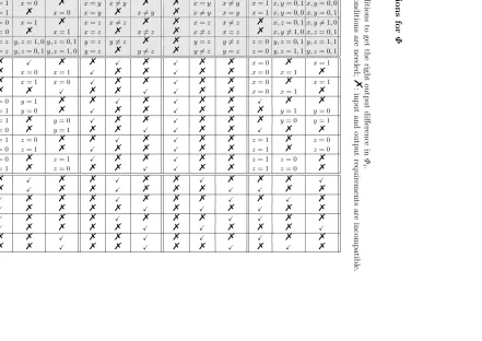
Interactions between the ∂-difference and the boolean functions. The main advantage of the signed difference∂over the modular differenceδis to handle the boolean function. The Φi’s are bitwise functions and we know for each bit how the input and
output are supposed to change betweenM andM′; if we add some conditions to restrict the inputs, we can make sure the output follows the path. See Table 3 in Appendix C for the full conditions.
Based on these tools, we will first show how to compute a set of sufficient conditions once a differential path is given. As such, it can be used to check a given differential path, and it will be the basis of our differential path search algorithm.
3.2 Computing a Set of Sufficient Conditions
The technique used here is rather simple, and is the same as [13]. This algorithm (referred to as SC algorithm) will take as input a message difference ∆ and a differential path h∂ii48i=0.
The SC algorithm will follow the path backwards fromQ48toQ0, and will recursively compute a set of conditions: at each step i, we assume that the current set is sufficient to satisfy the path from stepQi+1 to Q48, and we will add some conditions to extend it to stepi. If we look at step i+ 4for messages M andM′, we have:
Qi+4= (Qi⊞Φi+4(Qi+3, Qi+2, Qi+1)⊞mi+4⊞ki+4)≪si+4 Q′
i+4= (Q′i⊞Φi+4(Q′i+3, Q′i+2, Q′i+1)⊞m′i+4⊞ki+4)≪si+4
We know how to compute δi≫+4 = δ(Qi+4 ≫ si+4, Q′i+4 ≫ si+4) from δi+4 (see Section 3.1), and this will give a first set of conditions on Qi+4 (we call these conditions
≪-conditions). Then we will add some extra conditions so that the path is followed:
1. IfΦ′
i+4⊟Φi+4 =δi⊟δ≫i+4⊞∆i+4, thenδQi =δi, so we select a∂(Φi+4, Φ′i+4), and we can ensure it is followed by adding a few extra conditions on the inputs Qi+1,Qi+2, Qi+3 of Φi+4 (see Table 3). We call these conditions Φ-conditions.
2. Once we have δQi =δi, we only need a few extra conditions on Qi to get ∂Qi =∂i
by Theorem 1. We call these conditions ∂-conditions.
3.3 The Differential Path Search Algorithm
Our algorithm is based on the SC algorithm. The basic idea is to run the SC computation, but since we do not know δi nor δΦi, we will assume that δΦi = 0, which gives δi =
MAJcan absorb one input difference. Using this basic idea, we find a path with a non-zero difference inQ−4...Q−1, that is, a path leading to pseudo-collisions (this initial path is calledǫin the algorithm).
Then we will run another pass of the algorithm, but we will try to modify the path so as to lower the number of differences in theIV. In fact, we will have a set of pathsP, and every run will select a path, try to enhance it, and insert new paths in this set. This basic structure is described in Algorithm 1: we will make an extensive use of recursivity to explore the path space. This algorithm will be referred to as the DP algorithm.
Algorithm 1 Overview of the differential path search algorithm
1: functionPathfind
2: P ← {ǫ} ⊲ ǫis the path withδΦi= 0
3: loop
4: extractP fromP
5: Pathstep(P,ǫ,48) ⊲start search from last step
6: functionPathstep(P0,P,i) ⊲Extend pathP to stepi, followingP0
7: if i <0then
8: addP toP
9: else
10: for allpossible choiceP′do
11: PatchTarget(P0,P′,i)
12: functionPatchTarget(P0,P,i) ⊲ModifyP to fixIVdifferences in the end
13: for allpossible choiceP′do
14: PatchCarries(P0,P′,i)
15: functionPatchCarries(P0,P,i) ⊲Extend some carries to help the next steps
16: for allpossible choiceP′do
17: Pathstep(P0,P′,i−1)
Path representation. During the computation of a path, we represent the path as h∂Qii48i=0, where each ∂Qi is given as 32 values in {−1,0,+1}. However, between two
passes, this representation is almost useless: when we apply a local modification to a ∂Qi, the∂Qj’s for the rest of the path will become quite different.
Therefore we propose a new representation of the path: we will store hδΦii48i=0. The
∂Qi’s can be efficiently computed from the δΦi’s, even if there is a little loss of
infor-mation: a given hδΦii48i=0 can correspond to many h∂ii48i=0 (for instance using different carry extensions), but the algorithm quickly finds a good one. The main advantage of this representation is that a local modification ofδΦi will not modify the other δΦj, and
we recompute the full path h∂Qii48i=0. In fact, since ∂Φi = 0 most of the time, this is a
much better description of the path: it tells us where we have to do something unusual.
Overview of the algorithm. The function Pathstep will extend the path one step
further, using the same ideas as the SC algorithm at step i+ 4. It assumes the ∂Qj’s
δQi from ∂Qi+4 and ∂Φi+4 and add the≪-conditions and Φ-conditions. It will have to choose a ∂Φi+4 matching δΦi+4 that is feasible given∂Qi+1,∂Qi+2, and ∂Qi+3; if none is available, this branch of the search is aborted. Here we will also setδΦi to the value it
had in the path P0, so that the new path is similar the old one.
The function PatchTarget will then modify ∂Φi so as to remove some unwanted
differences in theIV (trying to turn a pseudo-collision path into a collision path). To finish the step i, the function PatchCarries will select a ∂Qi corresponding to
δQi, and will extend some carries according to the values δΦi+1,δΦi+2 and δΦi+3. This step is important because we need a non-zero bit in a∂Qj−1,∂Qj−2 or ∂Qj−3 for every non-zero bit in∂Φj. Then it will add the∂-conditions.
Correcting Differences. The critical part of the algorithm is the computation of the bits to modify in step iso as to correct a difference in the IV. To change directly a bit Q[ik0], we will set a non-zero difference in Φ[k⊟si0]
i0 . However, we detect the differences in
theIV, and we can’t fix them here; we will have to act on a different step and see how the difference evolves. The simplest way to do so is to keep δΦi unmodified in the rest
of the path, which is possible if the difference is absorbed by theΦi’s. So we will try to
use bit Q[k⊞si0]
i0+4 to modify bitQ
[k]
i0, and so on until we find a bit of Qi0+4t which can be
changed usingΦ.
When such a modification succeeds, it will remove one difference in the IV. This simple correction method is already useful: it finds the path from [23], but not the one from [19].
Indirect Correction. While searching for more complex paths, we will have some differences in theIVwhich cannot be dealt with this way. So we will introduce a difference which will not directly cancel the difference in theIV, but which will allow us to remove the target difference using the previous method. More precisely, to fix Q[ik0], we want a difference in someQi0+4t, but we need a difference in the inputs ofΦi0+4t; so we will try
to introduce a difference in Qi0+4t+a, where a∈ {1,2,3}, and this will use Φi0+4t+a+4t′.
See Algorithm 2 for a pseudo-code description.
When this succeeds, it removes the target difference, but it introduces a new un-wanted difference. Hopefully, we may remove this new difference without indirect mod-ifications... This method works rather well, and finds many paths using the message difference from [19].
Impossible paths. As we compute the differential path and the sufficient conditions at the same time, we do not have to deal with impossible path, during the execution of the algorithm: if a modification of the paths leads to an impossibility, we abort the search and look for other modifications. However, if the path with δΦi = 0 is impossible – and
this is the case if there are some differences in the third round1 – the first pass of the
1 for Wang’s EUROCRYPT path, the differences in the third round form a local collisions, so we can
Algorithm 2 Details on the bit correcting part of the algorithm
1: functionPatchTarget(P0,P,i)
2: for allQ[ik0] bit to fix inP0do ⊲we try every difference, one by one
3: PatchTargetBit(P0,P,i,i0,k,η0)
4: functionPatchTargetBit(P0,P,i,i0,k,η) ⊲ η indirect modifications allowed
5: if i < i0 then return
6: else if i=i0 then
7: modifyP on bitk of stepi
8: PatchCarries(P0, P, i) ⊲next step of the algorithm
9: else
10: PatchTargetBit(P0, P, i, i0+ 4, k+si0 mod 32, η) ⊲Direct correction
11: if η >0then
12: modifyP0 on bitkof stepi0 ⊲Indirect correction
13: fora∈ {1,2,3}doPatchTargetBit(P0,P,i,i0+a,k,η−1)
algorithm will abort with an incomplete path. Therefore we also add incomplete paths to the set P, and we correct their errors in the same ways we correct differences in the IV.
Exploring the search space. In order to avoid spending too much time on uninterest-ing paths, we have to choose an interestuninterest-ing path in the setP. As the indirect corrections are much expensive that direct ones, we only search for them on paths that have already been run without indirect corrections, and we favour runs without indirect corrections. We implemented the set P as a priority queue, and our priority function is based on:
– the number of difference in the IV – the number of conditions
– the number of indirect correction allowed
– the depth in the tree (ie. the number of run between the first path and the current path)
To restrict the search space, we also set some limits on the path we are looking for. The difficulty here is to keep enough paths to find the good ones, while cutting enough branches in the search tree to finish in reasonable time. In our algorithm, we limit the size of the carries, and the number of total conditions in a path. We also limit the total number of runs of the algorithm, which allows to keep the set P to a fixed size.
Example. See Table 2 in Appendix B for an example of how the algorithm modifies the paths until it has noIVdifference. For this path, there is no need for indirect correction.
3.4 Comparison with Existing Algorithms
the basic idea that rules the algorithm is not the same. Schläffer and Oswald basically try to cancel the differences introduced in the message, while we basically try to compute Qi for Qi+1...Qi+4. Our approach computes the path and the sufficient conditions at the same time, whereas Schläffer and Oswald performed these two steps separately, and had to deal with impossible paths. A more important innovation from our algorithm comes from the possibility of indirect corrections: Oswald and Schläffer had to manually introduce disturbance difference which seemed to play the same role. It seems that the general structure of their algorithm is not well suited to automate this part. As a result our algorithm finds better ways to choose the indirect corrections, which results in a much better path.
De Cannière and Rechberger [2]. This work introduces some important new ideas, and some of them could be used to enhance our algorithm (eg. the generalised differential ∇). However their algorithm as such does not seem really suitable for MD4. It seems that they are only doing local modification to the path, and they can’t correct a difference far from were it was introduced. This feature is well adapted to MD5, SHA-0 and SHA-1 because the step update function will duplicate a difference in the internal state. In MD4, a difference can be absorbed by theΦi’s, and we can correct it many steps further.
Furthermore, the basic idea of iteratively adding conditions seems incompatible with our indirect modification scheme.
Sasaki [15]. Sasaki introduces an interesting idea in FSE ’07 [15]: he combines forward search and backward search with a meet-in-the-middle approach. We believe this can be adapted to our algorithm but we didn’t had the time to do it yet. More importantly, Sasaki introduces a new message difference and a correspond path. Our algorithm does not work yet with this message difference, but we are working on it.
4 Applications
The algorithm was implemented in the C language, and we ran it with different message differences on a desktop computer. We used it to check the paths given by Wang et al.
in [19] and [23].
4.1 Yu et al.’s CANS Path [23]
By applying our algorithm to Yuet al.’s CANS path [23], we found that
– This path is rather easy to find and does not require any indirect modifications. Our algorithm finds it in about 0.1 s.
– In [23], the authors claim that the path can be rotated and gives 32 similar paths using a message difference on the different bits of Q4, but only 28 paths are actually correct2.
– If the difference is applied to bit 25 instead of bit 22, the path has only 58 conditions instead of 62. This is good news for applications where one only needs one path with the smallest possible number of conditions, such as attacks against NMAC-MD4 [7,4].
4.2 Wang’s EUROCRYPT Path [19]
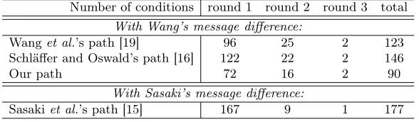
We also ran our algorithm with the message difference of Wang’s EUROCRYPT path [19], and we found many paths with less conditions; the two best are detailed in Path 1 and Path 2. These paths are much harder to find: they need some indirect modifications, and our algorithm takes a few hours to find them (however, a first solution is found in a few minutes, and it already has only 19 conditions on the second round). Our path is also better than the one found by Oswald and Schläffer, see Table 1 for a quick comparison. The number of conditions in a path determines the complexity of the collisions finding phase: conditions in the first round cost almost nothing (because message modification in the first round always succeeds); in the beginning of the second round, they cost a little bit more; and in the end of the second round and in the last round they can only be fulfilled statistically, so they have an exponential cost.
Table 1: Comparison of paths using the same message difference
Number of conditions round 1 round 2 round 3 total
With Wang’s message difference:
Wanget al.’s path [19] 96 25 2 123
Schläffer and Oswald’s path [16] 122 22 2 146
Our path 72 16 2 90
With Sasaki’s message difference:
Sasakiet al.’s path [15] 167 9 1 177
As far as MD4 collisions are concerned, the best path currently known is due do Sasaki et al. [15] and uses another message difference. Unfortunately, we have not yet been able to make our algorithm work with this message difference.
4.3 IV-dependent differential path
exhaustive search over the remainingIV bits, and we can easily check the validity of the IV using the collisions found.
IV-dependent differential paths can be used to attack some MAC algorithms, in particular NMAC/HMAC.
Our algorithm found 22 IV-dependent paths with a one-bit difference∆0 = 2k. Path 4 in Appendix B shows one of them withk= 0, and the other ones are obtained with a bit rotation of the whole path. They have one condition on the IV: Q[k⊞s0]
−1 =Q
[k⊞s0]
−2 , and 79 conditions on the other internal state variables.
Conclusion and outlook
Our algorithm is successful at finding differential paths with some given message differ-ential. Our paths have fewer conditions than the previously known ones, which shows that our algorithm is efficient. Good paths are not really needed for collision search, since collisions are already very cheap, but we believe that new kinds of attack against MD4 or MD4-based constructions could be found thanks to this algorithm. New differential paths could led to new attacks.
We are trying to explore what can be done with various differential paths, and we have already found a full key-recovery attack against NMAC-MD4 based on IV-dependent path.
References
1. John Black, Martin Cochran, and Trevor Highland. A Study of the MD5 Attacks: Insights and Improvements. In Robshaw [12], pages 262–277.
2. Christophe De Cannière and Christian Rechberger. Finding SHA-1 Characteristics: General Results and Applications . In Lai and Chen [10].
3. Anne Canteaut, editor. Ongoing research areas in symmetric cryptography. Technical Report
D.STVL.3, ECRYPT, 2005. http://www.ecrypt.eu.org/documents/D.STVL.3-2.5.pdf.
4. Scott Contini and Yiqun Lisa Yin. Forgery and Partial Key-Recovery Attacks on HMAC and NMAC Using Hash Collisions. In Lai and Chen [10].
5. Ronald Cramer, editor. Advances in Cryptology - EUROCRYPT 2005, 24th Annual International Conference on the Theory and Applications of Cryptographic Techniques, Aarhus, Denmark, May 22-26, 2005, Proceedings, volume 3494 ofLecture Notes in Computer Science. Springer, 2005. 6. M. Daum. Cryptanalysis of Hash Functions of the MD4-Family. PhD thesis, Ruhr-University of
Bochum, 2005.
7. Jongsung Kim, Alex Biryukov, Bart Preneel, and Seokhie Hong. On the Security of HMAC and NMAC Based on HAVAL, MD4, MD5, SHA-0 and SHA-1. In Roberto De Prisco and Moti Yung, editors,SCN, volume 4116 ofLecture Notes in Computer Science, pages 242–256. Springer, 2006. 8. Vlastimil Klima. Finding MD5 Collisions on a Notebook PC Using Multi-message Modifications.
Cryptology ePrint Archive, Report 2005/102, 2005. http://eprint.iacr.org/.
9. Vlastimil Klima. Tunnels in Hash Functions: MD5 Collisions Within a Minute. Cryptology ePrint Archive, Report 2006/105, 2006. http://eprint.iacr.org/.
10. Xuejia Lai and Kefei Chen, editors. 12th International Conference on the Theory and Application of Cryptology and Information Security, Shanghai, China, December 3-7, 2006. , volume 4284 of
Lecture Notes in Computer Science. Springer, 2006.
11. Yusuke Naito, Yu Sasaki, Noboru Kunihiro, and Kazuo Ohta. Improved Collision Attack on MD4 with Probability Almost 1. In Dongho Won and Seungjoo Kim, editors, ICISC, volume 3935 of
12. Matthew Robshaw, editor.Fast Software Encryption: 13th InternationalWorkshop, FSE 2006 Graz, Austria, March 15-17, 2006 Revised Selected Papers, volume 4047 of Lecture Notes in Computer Science. Springer, 2006.
13. Yu Sasaki, Yusuke Naito, Jun Yajima, Takeshi Shimoyama, Noboru Kunihiro, and Kazuo Ohta. How to Construct Sufficient Condition in Searching Collisions of MD5. In Phong Q Nguyen, editor,
VIETCRYPT, volume 4341 ofLecture Notes in Computer Science. Springer, 2006.
14. Yu Sasaki, Lei Wang, Kazuo Ohta, and Noboru Kunihiro. Extended APOP Password Recovery Attack. Presented at the rump session of FSE ’07. http://fse2007.uni.lu/rump.html.
15. Yu Sasaki, Lei Wang, Kazuo Ohta, and Noboru Kunihiro. New Message Difference for MD4, 2007. To appear in FSE ’07 proceedings.
16. Martin Schläffer and Elisabeth Oswald. Searching for Differential Paths in MD4. In Robshaw [12], pages 242–261.
17. Victor Shoup, editor.Advances in Cryptology - CRYPTO 2005: 25th Annual International Cryptol-ogy Conference, Santa Barbara, California, USA, August 14-18, 2005, Proceedings, volume 3621 of
Lecture Notes in Computer Science. Springer, 2005.
18. Marc Stevens. Fast Collision Attack on MD5. Cryptology ePrint Archive, Report 2006/104, 2006.
http://eprint.iacr.org/.
19. Xiaoyun Wang, Xuejia Lai, Dengguo Feng, Hui Chen, and Xiuyuan Yu. Cryptanalysis of the Hash Functions MD4 and RIPEMD. In Cramer [5], pages 1–18.
20. Xiaoyun Wang, Yiqun Lisa Yin, and Hongbo Yu. Finding Collisions in the Full SHA-1. In Shoup [17], pages 17–36.
21. Xiaoyun Wang and Hongbo Yu. How to Break MD5 and Other Hash Functions. In Cramer [5], pages 19–35.
22. Xiaoyun Wang, Hongbo Yu, and Yiqun Lisa Yin. Efficient Collision Search Attacks on SHA-0. In Shoup [17], pages 1–16.
23. Hongbo Yu, Gaoli Wang, Guoyan Zhang, and Xiaoyun Wang. The Second-Preimage Attack on MD4. In Yvo Desmedt, Huaxiong Wang, Yi Mu, and Yongqing Li, editors,CANS, volume 3810 of
Lecture Notes in Computer Science, pages 1–12. Springer, 2005.
A Interaction between modular difference and rotation
Leta, b∈Z232,0≤s <32 andα=a≪s, β =b≪s. We want to computeυ=δ(α, β)
from u = δ(a, b) and a. We will use the integer addition + (in Z) and the modular addition⊞(in Z232), and we express the rotation in the following way:
x≪s= (2sxmod 232) +
xmod 232 232−s
.
We will use the following result on integer part:
⌊x+y⌋= (
If a+u <232(in Z), then:
β−α= a+u 232−s
+ 2s(a+u)
− j
a 232−s
k +2sa
=
a+u 232−s
−j a 232−s
k + 2su
=j u 232−s
k
+ 2su or j u 232−s
k
+ 2su+ 1
β⊟α=u≪s or (u≪s)⊞1
Otherwise, 232≤a+u <233:
β−α= a+u−2 32
232−s
+ 2s(a+u)
−
j a
232−s
k + 2sa
=−2s+ a+u 232−s
+ 2s(a+u)
−
j a
232−s
k + 2sa
β⊟α= (u≪s)⊟2s or (u≪s)⊟2s⊞1
Furthermore, we can explicit precise conditions for each case:
υ=
υ1 = (u≪s) if a+u <232 and
(amod 232−s) + (umod 232−s)<232−s
υ2 = (u≪s)⊞1 if a+u <232 and
(amod 232−s) + (umod 232−s)≥232−s
υ3 = (u≪s)⊟2s if a+u≥232 and
(amod 232−s) + (umod 232−s)<232−s
υ4 = (u≪s)⊟2s⊞1if a+u≥232 and
(amod 232−s) + (umod 232−s)≥232−s
B Differential Paths
All the paths given in this section will use the notations defined in the article. Moreover, there are two extra differences with Wang’s tables:
– The ∂-conditions are not included in the table, since they can be easily be deduced from ∂i (eg. Q[6]1 = 1 in step 1 of Path 1).
Path 1: First of the two best paths we found with the same message difference as [19].
step si δmi ∂Φi ∂Qi Φ-conditions and≪-conditions
0 3 1 7 ˙
N[31]¸ ˙
H[6]¸ 2 11˙
H[28],N[31]¸ ˙
NNN[7...9]¸
Q[6]0 =Q[6]−1
3 19 Q[6]2 = 0,Q[7]1 =Q[7]0 ,Q[8]1 =Q[8]0 ,Q[9]1 =Q[9]0
4 3 ˙
H[6]¸ ˙
NH[9,10]¸
Q[6]3 = 0,Q[7]3 = 0,Q[8]3 = 0,Q[9]3 = 0 5 7 ˙
N[7]¸ ˙
N[13]¸
Q[7]4 = 0,Q [8] 4 = 1,Q
[9] 3 = 0,Q
[10] 3 =Q
[10] 2
6 11 ˙
H[10]¸ ˙
H[18]¸
Q[9]5 = 0,Q [10] 5 = 1,Q
[13] 4 =Q
[13] 3
7 19 Q[9]6 = 1,Q [10] 6 = 1,Q
[13] 6 = 0,Q
[18] 5 =Q
[18] 4
8 3 ˙
N[13]¸ ˙
H[12],HN[16,17]¸
Q[13]7 = 0,Q [18] 7 = 0
9 7 ˙
H[12]¸ ˙
N[19]¸
Q[12]7 = 1,Q [12] 6 = 0,Q
[16] 7 =Q
[16] 6 ,Q
[17] 7 =Q
[17] 6 ,Q
[18] 8 = 1
10 11 ˙
N[17]¸ ˙
H[28]¸
Q[12]9 = 0,Q[16]9 = 0,Q[17]9 = 1,Q[19]8 =Q[19]7
11 19 Q[12]10 = 1,Q[16]10 = 1,Q[17]10 = 1,Q[19]10 = 0,Q[28]9 =Q[28]8
12 3 ˙
H[16]¸ ˙
N[19]¸ ˙
H[15],N[22]¸
Q[19]11 = 0,Q[28]11 = 0
13 7 ˙
HHN[26...28]¸
Q[15]11 =Q [15] 10 ,Q
[22] 11 =Q
[22] 10 ,Q
[28] 12 = 1
14 11 ˙
N[28]¸
Q[15]13 = 0,Q [22] 13 = 0,Q
[26] 12 =Q
[26] 11 ,Q
[27] 12 =Q
[27] 11 ,Q
[28] 12 = 1,Q
[28] 11 = 0
15 19 ˙
N[28]¸ ˙
N[15]¸
Q[15]14 = 1,Q [22] 14 = 1,Q
[26] 14 = 0,Q
[27] 14 = 0,Q
[28] 14 = 1
16 3 ˙
N[15]¸ ˙
N[25]¸
Q[15]14 6=Q[15]13 ,Q[26]15 =Q[26]14 ,Q[27]15 =Q[27]14 ,Q[28]15 =Q[28]14
17 5 ˙
N[31]¸
Q[15]16 =Q [15] 14 ,Q
[25] 15 =Q
[25] 14
18 9 Q[15]17 =Q [15] 16 ,Q
[25] 17 =Q
[25] 15 ,Q
[31] 16 =Q
[31] 15
19 13 ˙
H[16]¸ ˙
H[28]¸
Q[25]18 =Q [25] 17 ,Q
[31] 18 =Q
[31] 16
20 3 ˙
N[31]¸ ˙
H[28],N[31]¸ ˙
N[28],H[31]¸
Q[28]18 6=Q [28] 17 ,Q
[31] 19 6=Q
[31] 18
21 5 ˙
H[31]¸
Q[31]19 6=Q[31]18
22 9 Q[31]21 =Q[31]19
23 13 ˙
N[28]¸
Q[28]22 6=Q[28]21 ,Q[31]22 =Q[31]21
24 3 ˙
H[28],N[31]¸ 25 5 26 9 27 13 28 3 29 5 30 9 31 13 32 3 33 9 34 11 35 15 ˙
H[16]¸ ˙
H[31]¸ 36 3 ˙
H[28],N[31]¸ ˙
H[31]¸ ˙
H[31]¸ 37 9
38 11
39 15 ˙
N[31]¸ 40 3 ˙
N[31]¸ 41 9 42 11 43 15 44 3 45 9 46 11 47 15
Path 2: Second of the two best paths found with the same message difference as [19].
step si δmi ∂Φi ∂Qi Φ-conditions and≪-conditions
0 3 1 7 ˙
N[31]¸ ˙
N[6]¸ 2 11˙
H[28],N[31]¸ ˙
H[7],N[10]¸
Q[6]0 =Q[6]−1
3 19 Q[6]2 = 0,Q[7]1 =Q[7]0 ,Q[10]1 =Q[10]0
4 3 ˙
NH[6,7]¸ ˙
NNH[9...11]¸
Q[6]3 = 0,Q[7]3 = 1,Q[10]3 = 0
5 7 ˙
N[13]¸
Q[7]4 = 1,Q [9] 3 =Q
[9] 2 ,Q
[10] 3 = 0,Q
[11] 3 =Q
[11] 2
6 11 ˙
NH[10,11]¸ ˙
H[18]¸
Q[9]5 = 0,Q [10] 5 = 1,Q
[11] 5 = 1,Q
[13] 4 =Q
[13] 3
7 19 Q[9]6 = 1,Q [10] 6 = 1,Q
[11] 6 = 1,Q
[13] 6 = 0,Q
[18] 5 =Q
[18] 4
8 3 ˙
N[13]¸ ˙
H[12],N[16]¸
Q[13]7 = 0,Q [18] 7 = 0
9 7 ˙
H[12]¸ ˙
N[19]¸
Q[12]7 = 1,Q [12] 6 = 0,Q
[16] 7 =Q
[16] 6 ,Q
[18] 8 = 1
10 11 ˙
H[29]¸
Q[12]9 = 0,Q[16]9 = 0,Q[19]8 =Q[19]7
11 19 Q[12]10 = 1,Q[16]10 = 1,Q[19]10 = 0,Q[29]9 =Q[29]8
12 3 ˙
H[16]¸ ˙
N[19]¸ ˙
H[15],N[22]¸
Q[19]11 = 0,Q[29]11 = 0
13 7 ˙
HHHN[26...29]¸
Q[15]11 =Q [15] 10 ,Q
[22] 11 =Q
[22] 10 ,Q
[29] 12 = 1
14 11 ˙
N[29]¸
Q[15]13 = 0,Q [22] 13 = 0,Q
[26] 12 =Q
[26] 11 ,Q
[27] 12 =Q
[27] 11 ,Q
[28] 12 =Q
[28] 11 ,Q
[29] 12 = 1,Q
[29] 11 = 0
15 19 ˙
HN[28,29]¸ ˙
N[15]¸
Q[15]14 = 1,Q [22] 14 = 1,Q
[26] 14 = 0,Q
[27] 14 = 0,Q
[28] 14 = 1,Q
[29] 14 = 1
16 3 ˙
N[15]¸ ˙
N[25]¸
Q[15]14 6=Q[15]13 ,Q[26]15 =Q[26]14 ,Q[27]15 =Q[27]14 ,Q[28]15 =Q[28]14 ,Q[29]15 =Q[29]14
17 5 ˙
N[31]¸
Q[15]16 =Q [15] 14 ,Q
[25] 15 =Q
[25] 14
18 9 Q[15]17 =Q [15] 16 ,Q
[25] 17 =Q
[25] 15 ,Q
[31] 16 =Q
[31] 15
19 13 ˙
H[16]¸ ˙
H[28]¸
Q[25]18 =Q [25] 17 ,Q
[31] 18 =Q
[31] 16
20 3 ˙
N[31]¸ ˙
H[28],N[31]¸ ˙
N[28],H[31]¸
Q[28]18 6=Q [28] 17 ,Q
[31] 19 6=Q
[31] 18
21 5 ˙
H[31]¸
Q[31]19 6=Q[31]18
22 9 Q[31]21 =Q[31]19
23 13 ˙
N[28]¸
Q[28]22 6=Q[28]21 ,Q[31]22 =Q[31]21
24 3 ˙
H[28],N[31]¸ 25 5 26 9 27 13 28 3 29 5 30 9 31 13 32 3 33 9 34 11 35 15 ˙
H[16]¸ ˙
H[31]¸ 36 3 ˙
H[28],N[31]¸ ˙
H[31]¸ ˙
H[31]¸ 37 9
38 11
39 15 ˙
N[31]¸ 40 3 ˙
N[31]¸ 41 9 42 11 43 15 44 3 45 9 46 11 47 15
Path 3: Improved version of the path from Yuet al. [23].
stepsi δmi ∂Φi ∂Qi conditions
0 3 1 7 2 11 3 19 4 3 ˙
N[25]¸ ˙
N[28]¸
5 7 Q[28]3 =Q[28]2
6 11 Q[28]5 = 0 7 19 Q[28]6 = 1 8 3 ˙
N[31]¸
9 7 Q[31]7 =Q [31] 6
10 11 ˙
N[31]¸ ˙
H[10]¸
Q[31]9 = 1
11 19 Q[10]9 =Q [10] 8 ,Q
[31] 10 = 1
12 3 ˙
N[2]¸
Q[10]11 = 0
13 7 Q[2]11=Q [2] 10,Q
[10] 12 = 1
14 11 ˙
H[21]¸ Q[2]13= 0
15 19 Q[2]14= 1,Q[21]13 =Q[21]12
16 3 ˙
N[5]¸
Q[21]15 =Q [21] 13
17 5 ˙
N[25]¸ ˙
N[5]¸ ˙
N[10],N[30]¸
Q[5]156=Q [5] 14,Q
[21] 16 =Q
[21] 15
18 9 ˙
H[30]¸ Q[5]17=Q[5]15,Q16[10]=Q[10]15 ,Q[30]16 =Q[30]15
19 13 Q[5]18=Q [5] 17,Q
[10] 18 =Q
[10] 16
20 3 ˙
N[8]¸
Q[10]19 =Q [10] 18
21 5 ˙
H[30]¸ ˙
N[15]¸
Q[8]19=Q [8] 18,Q
[30] 20 6=Q
[30] 19
22 9 ˙
NH[7,8]¸
Q[8]21=Q [8] 19,Q
[15] 20 =Q
[15] 19
23 13 Q[7]21=Q [7] 20,Q
[15] 22 =Q
[15] 20
24 3 ˙
H[8]¸
Q[7]23=Q [7] 21,Q
[8] 236=Q
[8] 21,Q
[15] 23 =Q
[15] 22
25 5 ˙
N[20]¸ Q[7]24=Q [7] 23,Q
[8] 24=Q
[8] 23
26 9 ˙
H[16]¸ Q[20]24 =Q[20]23
27 13 Q[16]25 =Q [16] 24 ,Q
[20] 26 =Q
[20] 24
28 3 Q[16]27 =Q [16] 25 ,Q
[20] 27 =Q
[20] 26
29 5 ˙
N[25]¸
Q[16]28 =Q [16] 27
30 9 ˙
H[25]¸
Q[25]28 =Q [25] 27
31 13 32 3
33 9 ˙
H[25]¸
Q[25]32 =Q [25] 31
34 11˙
N[25]¸ 35 15 36 3 37 9 38 11 39 15 40 3 41 9 42 11 43 15 44 3 45 9 46 11 47 15
Path 4: An IV-dependent path with the message difference on the first word.
step si δmi ∂Φi ∂Qi Φ-conditions and≪-conditions
0 3 ˙
N[0]¸ ˙
N[3]¸
1 7 Q[3]−1=Q [3]
−2
2 11 Q[3]1 = 0 3 19 Q[3]2 = 1
4 3 ˙
HN[6,7]¸
5 7 Q[6]3 =Q [6] 2 ,Q
[7] 3 =Q
[7] 2
6 11 Q[6]5 = 0,Q [7] 5 = 0
7 19 ˙
N[7]¸ ˙
N[26]¸
Q[6]6 = 1,Q [7] 6 = 0
8 3 ˙
H[26]¸ ˙
N[9],H[29]¸
Q[26]5 = 1,Q [26] 6 = 0
9 7 Q[9]7 =Q [9] 6 ,Q
[26] 8 = 0,Q
[29] 7 =Q
[29] 6
10 11 Q[9]9 = 0,Q [26] 9 = 1,Q
[29] 9 = 0
11 19 ˙
N[13]¸
Q[9]10= 1,Q[29]10 = 1 12 3 ˙
H[0],N[12]¸ Q[13]10 =Q[13]9
13 7 Q[0]11=Q [0] 10,Q
[12] 11 =Q
[12] 10 ,Q
[13] 12 = 0
14 11 ˙
H[0]¸ ˙
NNH[11...13]¸
Q[0]13= 1,Q [12] 13 = 0,Q
[13] 13 = 1
15 19 ˙
H[13]¸
Q[0]14= 1,Q [11] 13 =Q
[11] 12 ,Q
[12] 13 = 0,Q
[13] 13 = 1,Q
[13] 12 = 0
16 3 ˙
N[0]¸ ˙
NH[12,13]¸
Q[11]15 =Q [11] 13 ,Q
[12] 15 6=Q
[12] 13 ,Q
[13] 15 6=Q
[13] 13
17 5 Q[11]16 =Q [11] 15 ,Q
[12] 16 =Q
[12] 15 ,Q
[13] 16 =Q
[13] 15
18 9 ˙
NNNH[20...23]¸
19 13 Q[20]17 =Q [20] 16 ,Q
[21] 17 =Q
[21] 16 ,Q
[22] 17 =Q
[22] 16 ,Q
[23] 17 =Q
[23] 16
20 3 ˙
H[23]¸ ˙
H[26]¸
Q[20]19 =Q [20] 17 ,Q
[21] 19 =Q
[21] 17 ,Q
[22] 19 =Q
[22] 17 ,Q
[23] 19 6=Q
[23] 17
21 5 Q[20]20 =Q [20] 19 ,Q
[21] 20 =Q
[21] 19 ,Q
[22] 20 =Q
[22] 19 ,Q
[23] 20 =Q
[23] 19 ,Q
[26] 19 =Q
[26] 18
22 9 ˙
H[29]¸
Q[26]21 =Q [26] 19
23 13 Q[26]22 =Q[26]21 ,Q[29]21 =Q[29]20
24 3 ˙
NH[29,30]¸
Q[29]23 =Q[29]21
25 5 Q[30]23 =Q [30] 22
26 9 ˙
N[29]¸
Q[29]25 6=Q [29] 23 ,Q
[30] 25 =Q
[30] 23
27 13 Q[29]26 =Q [29] 25 ,Q
[30] 26 =Q
[30] 25
28 3 ˙
H[0]¸
29 5 Q[0]27=Q [0] 26
30 9 Q[0]29=Q [0] 27
31 13 Q[0]30=Q [0] 29
32 3 ˙
N[0]¸ 33 9 34 11 35 15 36 3 37 9 38 11 39 15 40 3 41 9 42 11 43 15 44 3 45 9 46 11 47 15
T ab le 2: E x am p le ru n on th e p at h fr om [1 9 ]. W e sh ow in te rm ed ia te st ep s to ea se co m -p re h en sio n , b u t th e al go rit h m ac tu al ly fi n d s fi n al d ir ec tly fr om th e or ig in al on e.
Initial path Path 1 Path 2 Path 3 Final Path
stepsi δmi ∂Φi ∂Qi ∂Φi ∂Qi ∂Φi ∂Qi ∂Φi ∂Qi ∂Φi ∂Qi
4 3 ˙
N[22]¸ ˙
H[22]¸ ˙
H[22]¸ ˙
H[22]¸ ˙
N[25]¸ ˙
N[25]¸
5 7 ˙
H[1],N[13]¸ ˙
H[8],N[20]¸ ˙
N[13]¸ ˙
N[20]¸ ˙
N[13]¸ ˙
N[20]¸ ˙
N[13]¸ ˙
N[20]¸
6 11 ˙
H[17]¸ ˙
H[28]¸ ˙
H[17]¸ ˙
H[28]¸
7 19
8 3 ˙
HN[28,29]¸ ˙
HN[28,29]¸
9 7 ˙
H[15],N[27]¸ ˙
N[27]¸ ˙
HN[27,28]¸ ˙
N[27]¸
10 11 ˙
H[7]¸ ˙
H[7]¸ ˙
H[28]¸ ˙
H[7]¸ ˙
H[28]¸ ˙
H[7]¸ ˙
H[28]¸ ˙
H[7]¸
11 19
12 3 ˙
N[31]¸ ˙
N[31]¸
13 7 ˙
N[2],H[22]¸ ˙
N[2]¸ ˙
N[2]¸ ˙
N[2]¸
14 11 ˙
H[18]¸ ˙
H[18]¸ ˙
H[18]¸ ˙
H[18]¸ ˙
H[18]¸
15 19
16 3 ˙
N[2]¸ ˙
N[2]¸
17 5 ˙
N[22]¸ ˙
N[7]¸ ˙
N[7],N[27]¸ ˙
N[7],N[27]¸ ˙
N[7],N[27]¸ ˙
N[2]¸ ˙
N[7],N[27]¸
18 9 ˙
H[27]¸ ˙
H[27]¸ ˙
H[27]¸ ˙
H[27]¸ ˙
H[27]¸
19 13
20 3 ˙
N[5]¸ ˙
N[5]¸
21 5 ˙
N[12]¸ ˙
H[27]¸ ˙
N[12]¸ ˙
H[27]¸ ˙
N[12]¸ ˙
H[27]¸ ˙
N[12]¸ ˙
H[27]¸ ˙
N[12]¸
22 9 ˙
H[4]¸ ˙
H[4]¸ ˙
H[4]¸ ˙
NH[4,5]¸ ˙
NH[4,5]¸
23 13
24 3 ˙
H[5]¸ ˙
H[5]¸
25 5 ˙
N[17]¸ ˙
N[17]¸ ˙
N[17]¸ ˙
N[17]¸ ˙
N[17]¸
26 9 ˙
H[13]¸ ˙
H[13]¸ ˙
H[13]¸ ˙
H[13]¸ ˙
H[13]¸
27 13 28 3
29 5 ˙
N[22]¸ ˙
N[22]¸ ˙
N[22]¸ ˙
N[22]¸ ˙
N[22]¸
30 9 ˙
H[22]¸ ˙
H[22]¸ ˙
H[22]¸ ˙
H[22]¸ ˙
H[22]¸
31 13 32 3
33 9 ˙
H[22]¸ ˙
H[22]¸ ˙
H[22]¸ ˙
H[22]¸ ˙
H[22]¸
34 11˙
C
C
o
n
d
it
io
n
s
fo
r
Φ
T
ab
le
3:
C
on
d
it
io
n
s
to
ge
t
th
e
rig
h
t
ou
tp
u
t
d
iff
er
en
ce
in
Φ
i.
X
:
n
o
ex
tr
a
co
n
d
it
io
n
s
ar
e
n
ee
d
ed
;
%
:
in
p
u
t
an
d
ou
tp
u
t
re
q
u
ir
em
en
ts
ar
e
in
co
m
p
at
ib
le
.
F(x, y, z) = IF(x, y, z) G(x, y, z) = MAJ(x, y, z) H(x, y, z) =x⊕y⊕z I(x, y, z) =y⊕(x∨ ¬z)
∂x ∂y ∂z ∂F= 0 ∂F= 1 ∂F=−1 ∂G= 0∂G= 1∂G=−1 ∂H= 0∂H= 1∂H=−1 ∂I= 0 ∂I= 1 ∂I=−1
0 0 0 X % % X % % X % % X % %
0 0 +1 x= 1 x= 0 % x=y x6=y % % x=y x6=y x= 1 x, y= 0,1x, y= 0,0 0 0 −1 x= 1 % x= 0 x=y % x6=y % x6=y x=y x= 1 x, y= 0,0x, y= 0,1 0 +1 0 x= 0 x= 1 % x=z x6=z % % x=z x6=z % x, z= 0,1x, y6= 1,0 0 −1 0 x= 0 % x= 1 x=z % x6=z % x6=z x=z % x, y6= 1,0x, z= 0,1 +1 0 0 y=z y, z= 1,0y, z= 0,1 y=z y6=z % % y=z y6=z z= 0 y, z= 0,1y, z= 1,1
−1 0 0 y=z y, z= 0,1y, z= 1,0 y=z % y=6 z % y6=z y=z z= 0 y, z= 1,1y, z= 0,1
0 +1 +1 % X % % X % X % % x= 0 % x= 1
0 −1 +1 % x= 0 x= 1 X % % X % % x= 0 x= 1 % 0 +1−1 % x= 1 x= 0 X % % X % % x= 0 % x= 1
0 −1−1 % % X % % X X % % x= 0 x= 1 %
+1 0 +1 y= 0 y= 1 % % X % X % % X % %
−1 0 +1 y= 1 y= 0 % X % % X % % % y= 1 y= 0 +1 0 −1 y= 1 % y= 0 X % % X % % % y= 0 y= 1
−1 0 −1 y= 0 % y= 1 % % X X % % X % %
+1 +1 0 z= 1 z= 0 % % X % X % % z= 1 % z= 0
−1 +1 0 z= 0 z= 1 % X % % X % % z= 1 % z= 0 +1−1 0 z= 0 % z= 1 X % % X % % z= 1 z= 0 %
−1−1 0 z= 1 % z= 0 % % X X % % z= 1 z= 0 %
+1 +1 +1 % X % % X % % X % % % X
−1 +1 +1 % X % % X % % % X X % %
+1−1 +1 X % % % X % % % X % X %
−1−1 +1 X % % % % X % X % X % %
+1 +1−1 X % % % X % % % X X % %
−1 +1−1 X % % % % X % X % % % X
+1−1−1 % % X % % X % X % X % %
![Table 2: Example run on the path from [19]. We show intermediate steps to ease com-](https://thumb-us.123doks.com/thumbv2/123dok_us/1856289.1241048/19.595.237.710.91.507/table-example-run-path-intermediate-steps-ease-com.webp)