Abstract
LIPMAN, DARREN SEITZ. Ties That Don’t Bind: Computing the Unknotting Numbers of Knot Families. (Under the direction of Dr. Radmila Sazdanovic.)
Computing the unknotting number of knots is generally a difficult and complex pursuit. To explore this challenge, we recall foundational concepts in knot theory, with a focus on the un-knotting number, Seifert surfaces, and knot signatures. We then discuss the BJ-unlinking num-ber and examine formulas derived by Jablan and Sazdanovic for computing the BJ-unlinking number, as well as the unknotting number, of knot families. Finally, we use explicit examples to illustrate how the established theory can be used to prove these formulas.
©Copyright 2016 by Darren Seitz Lipman
Ties That Don’t Bind: Computing the Unknotting Numbers of Knot Families
by
Darren Seitz Lipman
A thesis submitted to the Graduate Faculty of North Carolina State University
in partial fulfillment of the requirements for the Degree of
Master of Science
Mathematics
Raleigh, North Carolina 2016
APPROVED BY:
Dr. Andrew Cooper Dr. Molly Fenn
Biography
Darren Lipman grew up in Asheboro, North Carolina, where he was homeschooled until gradu-ating high school. He attended Guilford Technical Community College in Jamestown, NC, where he obtained his associate degree and served as president of both the Gay-Straight Alliance and the Student Government Association.
In 2012, Lipman transferred to North Carolina State University in Raleigh, NC, where he finished his bachelor’s degree in mathematics, with a second major in political science and a minor in creative writing. At NC State, he served as president of the GLBT Community Alliance, Alternative Service Break team leader for the 2015 San Francisco trip, and was awarded the 2015 Undergraduate Poetry Prize. He continued at NC State in the accelerated Master’s in Mathematics program, from which he graduated in May 2016.
Lipman will serve as a 2016 Teach for America corps member in Milwaukee, Wisconsin, where he plans to teach high school mathematics.
Acknowledgements
I cannot acknowledge anyone for my success in mathematics without first mentioning Mrs. Pam Coldwell, former Mathematics Department Head at Guilford Technical Community College, who first inspired my love and passion for mathematics, and Dr. Jay DeJohn, also of GTCC, whose calculus class made me commit myself to pursuing a major in mathematics.
Since transferring to North Carolina State University, I have had the fortune to learn under many amazing professors, and the following have had a significant influence on my growth and development as a mathematician: Dr. Molly Fenn, Dr. Alina Duca, Dr. Hoon Hong, Dr. Seth Sullivant, Dr. Sandra Paur, Dr. Min Kang, Dr. James Selgrade, and Dr. Andrew Cooper. Without their instruction and guidance, in the classroom and beyond, my experience at NC State and my interest in mathematics would have sorely suffered.
Dr. Megan Ryals, assistant director of the University Tutorial Center, deserves special recog-nition for her hand in developing my skills as a math tutor and for all the hours we spent discussing math, pedagogy, and math pedagogy, which no doubt played a substantial role in my decision to pursue education and my acceptance to Teach for America.
Most of all, I owe my greatest thanks to Dr. Radmila Sazdanovic. Her classes in topology reinvigorated my passion for mathematics, and her guidance as I began studying knot theory allowed me to grow as a mathematician in ways I hadn’t imagined possible. Her encouragement, confidence in me, and constant reminders to stay on task made all of this possible.
Table of Contents
LIST OF FIGURES . . . v
Chapter 1 Introduction . . . 1
Chapter 2 Knot Theory . . . 2
2.1 Knots and Links . . . 2
2.2 Knot Equivalence and Invariants . . . 5
2.3 Unknotting Number . . . 8
2.4 Seifert Surfaces . . . 12
2.5 Knot Signatures . . . 16
Chapter 3 Unknotting Numbers of Knot Families . . . 21
3.1 Conway Notation . . . 21
3.2 The BJ-Unlinking Number . . . 23
3.3 Unknotting the P[3,3,2] Pretzel Knot . . . 25
3.4 Formulas for Knot Families . . . 27
3.5 Conclusion . . . 31
LIST OF FIGURES
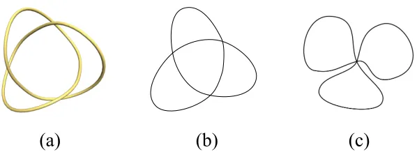
Figure 2.1 The Trefoil(31 in knot tables) is depicted as a 3D rendering (generated by
[17]) in (a), from which we can obtain a regular projection (b). In (c), the trefoil’s crossings have been moved to project onto the same point, making
this six-valent projection irregular. . . 3
Figure 2.2 Knot DiagramsAn irregular projection of 31giving the appearance of four crossings (a); an oriented knot diagram (b) and an alternative unoriented diagram (c) of 31. . . 3
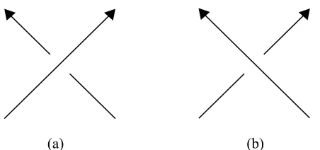
Figure 2.3 Signed Crossings(a) is positive while (b) is negative. . . 4
Figure 2.4 R1untwists a loop, decreasingc(D) by one. . . 6
Figure 2.5 R2moves one arc across another, decreasingc(D) by two. . . 6
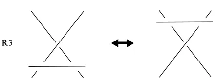
Figure 2.6 R3moves an arc across a crossing, leaving c(D) unchanged. . . 6
Figure 2.7 Unknotting the TrefoilA single crossing change unknots the trefoil. . . . 8
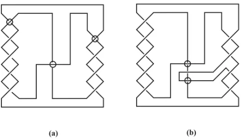
Figure 2.8 The Nakanashi-Bleiler Example The minimal knot diagram of 108 re-quires three simultaneous crossing changes (circled), but a diagram with one additional crossing (b) requires only two. Figure adapted from [7]. . . 10
Figure 2.9 n-crossing UnknotsThe 4-crossing diagram on the left is either ascending (if traced to the right of the starting point, circled) or descending (traced to the left). Using R1 and R2 moves, we see it is in fact the unknot. . . 11
Figure 2.10 Distinguishing Knots The unknotting number can distinguish the two knots with minimal crossing number 5. The necessary crossings to be changed have been circled; readers are encouraged to unknot 51 and 52 as an exercise (see Fig. 2.7). Knot diagrams are obtained from [13]. . . 12
Figure 2.11 Orientability of Two DisksIn (a), we see how the orientation of one disk determines that of the other. In (b), we see how nested disks must share the same upward-facing orientation. . . 14
Figure 2.12 Additional Seifert CirclesAdding a single disk to two nested disks forces an orientation in (a), but in (b), we see that adding a single disk to two nested disks allows for only one possible connection. . . 14
Figure 2.13 Kauffman Resolutions . . . 18
Figure 2.14 Seifert SurfacesSeifert surfaces for the knots 31(the trefoil), 41(the figure-eight), 52, and 61. The left column shows knot diagrams from [13]. The central and right columns show two possible Seifert surfaces for each knot generated by the free software SeifertView [17]. . . 20
Figure 3.1 Elementary TanglesThese correspond with signed crossings. . . 21
Figure 3.2 Tangle Operations (a) the construction of −T from T; (b) the sum of T and S, denoted t s; (c) the product ofT andS, denoted t, s. . . 22
Figure 3.3 P(3,3,2) (85 in knot tables) shown as a pretzel knot. . . 25
Figure 3.5 Seifert Matrix for P[3,3,2] V obtained from [13] and V0 computed using
[18]. Diagonal entries ofV0 were rounded to the nearest non-zero integer for clarity of presentation. . . 26 Figure 3.6 Kauffman Resolutions of P[3,3,2] Diagrams for the all-A (a) and all-B
(b) Kauffman resolutions. Positive and negative crossings (orientation not shown) have been marked. . . 26 Figure 3.7 Unknotting P[3,3,2] The two crossing changes that unknot P[3,3,2] are
cir-cled in the first diagram. Moving left-to-right, the strands moved between diagrams are color coded. . . 27 Figure 3.8 Unlinking R[3,3] By Theorem 3.4.1(1), we have thatu(R[3,3]) = 3+32 = 3.
The three crossings have been circled. . . 28 Figure 3.9 sA of R[2m+1,2n] In (a), we showR[3,2] can be oriented to have all negative
crossings so that sA= 3. In (b), we show the construction of a general
Chapter 1
Introduction
Knot theory is a rich area in the field of topology that studies embeddings of the circle S1
inR3. A key pursuit is finding methods of distinguishing different three-dimensional knots by studying their planar diagrams. In order to do this, we construct knot invariants that are values (such as numbers, polynomials, or algebraic structures) assigned to knots and knot diagrams in such a way that two diagrams of the same knot have the same value.
One invariant is the unknotting number, which counts the minimum number of crossing changes necessary to change the diagram of a knot into a diagram of the trivial knot, over all possible diagrams of the knot being considered.
However, the unknotting number is notoriously difficult to compute, and only a few families of knots have had their unknotting numbers computed in a general setting. One method of computing unknotting numbers is to find a lower and upper bound for the number, and if the lower bound can be realized, the unknotting number has been found. One method of finding a lower bound uses the signature of knot, which can be computed algebraically from geometric surfaces whose boundary is the knot and also by using combinatorial formulas.
In Chapter 2, we present an overview of fundamental concepts in knot theory. Section 2.1 begins with formal definitions of knots and their properties; Section 2.2 introduces knot equiva-lence and knot invariants; Section 2.3 establishes important concepts related to the unknotting number; Section 2.4 discusses Seifert surfaces, an integral step on the path to computing knot signatures; and finally Section 2.5 considers two possible methods of computing knot signatures, first through the use of Seifert surfaces and second through the use of formulas derived from a homological study of knots and links.
Chapter 2
Knot Theory
2.1
Knots and Links
We begin with a thorough introduction to knots, links, and their basic properties. The definitions and theorems about knots are presented as in Livingston [12] and Kauffman [9], both of which explore these topics with greater depth.
Definition 2.1.1. An n-component linkL is the embedding ofnnon-intersecting copies of the circle S1 in R3 (or S3). A knot K is a one-component link. A knot isotopic to S1 is called a trivial knot, or an unknot; a link isotopic to n copies of S1 is called the n component trivial link or unlink.
Working with knots and links in three-dimensional space is not impossible, but for those who prefer working with pencils and paper, exploring three-dimensional objects on a plane presents some critical difficulties that we would rather avoid. Therefore, we will develop a definition for knot diagrams, that is, planar depictions of knots and links.
For brevity, knots and links will be referred to as knots in the remainder of this section.
Definition 2.1.2. Given a knotK and a planeP, the knot projectionPK is a four-valent graph
obtained by projecting the knot K in R3 upon the planeP.
There is an infinite number of planes P upon which we can project the knotK, so a single knot may have any number of possible projections.
of precisely two points of K to a single point on the plane. In order to faithfully preserve the knot’s three-dimensional structure, we must mark the projection in such a way that it is clear which arc of the knot passes over the other inR3.
(a) (b) (c)
Figure 2.1: The Trefoil (31 in knot tables) is depicted as a 3D rendering (generated by [17])
in (a), from which we can obtain a regular projection (b). In (c), the trefoil’s crossings have been moved to project onto the same point, making this six-valent projection irregular.
Definition 2.1.3. A knot diagram D of a knot K is a projection PK of K with additional
crossing information; that is, at each vertex of PK, the projection is modified to show which
arc passes over the other. Such points are called the crossings of D, andc(D) is the number of crossings in the diagram D. If PK is regular, then the knot diagramD is regular.
There is a case in which two points in a knot may project onto the same point in the projection, but do not represent a crossing (see Fig. 2.2a). Should this happen, the two arcs that touch in the projection can be moved slightly apart in a continuous fashion inR3 so that the only pairs of points that project onto a single point represent actual crossings.
(a) (b) (c)
Figure 2.2: Knot Diagrams An irregular projection of 31 giving the appearance of four
Next, at times it is useful to consider a knot as a parametrized curve inR3. One motivation is that this will enable the construction of surfaces associated with the knot, a topic that will be considered later in this chapter. We now want to be able to draw knot diagrams that preserve this new information. In fact, if we trace the diagram in tandem with the knot’s parametrization, the diagram will inherit an orientation (see Fig 2.2b).
Definition 2.1.4. An oriented knot diagram is a knot diagram with a specified orientation.
One benefit of orienting a knot diagram is the ability to label its crossings as either positive or negative.
Definition 2.1.5. Let D be an oriented diagram for a knot K and let c be a crossing in D. Rotate the diagram (via planar isotopy or simply moving the paper in your hands) so that the orientation of the arcs in the crossing c point north-west and north-east, respectively. If the overcrossing passes from left to right, then sign(c) = +1, else sign(c) =−1.
See Fig. 2.3 for reference. In particular, signed crossings also allow us to define the writhe of a knot diagram, which can be used in various computations.
(a) (b)
Figure 2.3: Signed Crossings(a) is positive while (b) is negative.
Definition 2.1.6. LetD be as before. The number of positive crossings ofDis denotedc+ and
the number of negative crossings is denoted c−. The writhe ofD is w(D) =c+−c−.
Readers should be aware that the definition of positive and negative crossings varies among authors, including those cited in this paper. The benefit of this particular convention is that it allows the use of theright-hand rule to determine the sign of a crossing:
2. Bend your fingers to a ninety-degree angle such that your fingers point in the direction of the undercrossing’s orientation, turning your hand over if necessary.
3. If the thumb points upward from the diagram, the crossing is positive. 4. If the thumb points downward into the diagram, the crossing is negative.
Definition 2.1.7. Let Dbe an orientated knot diagram. Pick a point onD and follow the knot diagram in the positive direction. If the crossings alternate between being over- and undercross-ings (or vice versa), then D is an alternating diagram. A knot K is an alternating knot if it admits at least one alternating diagram.
The trefoil pictured in Fig. 2.2b,c is alternating (and, where oriented, each crossing is posi-tive). Note that an alternating knot can have non-alternating diagrams.
2.2
Knot Equivalence and Invariants
A fundamental question in knot theory is which knots are distinct and which are the same? However, it is sometimes preferable to work with knot diagrams than knots inR3, so we would like to determine knot equivalence by working solely with knot diagrams. For example, given diagramsD1 andD2, can we determine if the knots they represent,K1 andK2, are equivalent?
Recall that knots are embeddings of the circle S1 in R3. If one knot can be deformed continuously into another without self-intersection, we say these two knots are of the sameknot type; knots with the same knot type are said to be equivalent knots. Therefore, in order to work with knot diagrams, we must determine how deformations of a three-dimensional knot affect its diagram upon a fixed projection plane while preserving its knot type.
Deforming the knot in R3 without the knot passing through itself is known as ambient isotopy and can be represented by two types of moves on the level of knot diagrams. The first is planar isotopy, by which we move and deform the arcs of a knot sufficiently far from the crossings that the crossing information is unchanged. The second type of operation is a Reidemeister move that may increase, decrease, or preserve the number of crossings.
Definition 2.2.1. A Reidemeister move is an operation performed locally on a knot diagram
R1 R1
Figure 2.4: R1untwists a loop, decreasingc(D) by one.
R1 R2
Figure 2.5: R2moves one arc across another, decreasingc(D) by two.
R1 R 23
Figure 2.6: R3moves an arc across a crossing, leaving c(D) unchanged.
It should be noted that only the local area affected by each Reidemeister move has been shown in these diagrams; these arcs should be assumed to connect to a larger knot or link that has not been shown here. A diagram that does not admit any R1 moves that decrease the number of crossings and has no nugatory crossings is called areduced diagram. (Nugatory crossings look like R1 loops where the loop is a region of the knot possibly containing multiple crossings and arcs.)
Note also that the Reidemeister moves work in both directions; that is, while R1 can be used to untwist a loop, it can also be used to create a new loop (in either direction).
the level of knot diagrams and state an important theorem in knot theory.
Definition 2.2.2. Two diagrams Dα and Dβ are equivalent if there is a finite series of knot
diagrams Dα = D0, D1, ..., Dn−1, Dn = Dβ relating one to the other such that each Di is
obtained from Di−1 by a single Reidemeister move or planar isotopy.
Theorem 2.2.3 (Reidemeister’s Theorem). Two knots K1 and K2 are equivalent if the
dia-grams D1 and D2, representing K1 andK2, respectively, are equivalent diagrams.
In particular, suppose D1 and D2 are two knot diagrams obtained from two different
pro-jections of a single knot K. Intuitively, we can use planar isotopy and the three Reidemeister moves in succession to move betweenD1 and D2. However, it may be necessary toincrease the
number of crossings in the intermediate diagrams in order to do this.
Unfortunately, even a finite sequence can be arbitrarily large, so computing equivalence solely with Reidemeister moves is an inefficient approach to determining whether or not two diagrams represent the same knot. Therefore, we want to find more direct ways of distinguishing two knots than determining their diagrams’ equivalence.
Definition 2.2.4. A knot invariant is a map from the set of knot diagrams to some other set or algebraic structure (such as integers, polynomials, groups, etc.) such that the value of the map remains unchanged under each Reidemeister move.
Remark 2.2.5. Let f represent the map of some knot invariant and let D1 and D2 be the
diagrams corresponding to knots K1 and K2, respectively. If f(D1) 6= f(D2), then K1 is not
equivalent to K2 (that is,K1 is distinct from K2).
It is important to note that the converse of Remark 2.2.5 is not necessarily true: If f(D1) = f(D2), it may be that K1 and K2 have the same value under this map, but are still distinct
knots. For example, theminimal crossing number of a knot is the smallest number of crossings necessary to draw the knot’s diagram. However, while there are only one each of knots with minimal crossing numbers 3 and 4, there are many knots with minimal crossing number 5 and higher that share the value of this invariant but are actually distinct.
Definition 2.2.6. If a diagram for a knot K has exactly K’s minimal number of crossings, it is called a minimal diagram.
Commonly used knot tables often classify knots according to their minimal crossing numbers using a minimal diagram for each knot. As seen in Fig. 2.2, a single knot may have multiple minimal diagrams.
2.3
Unknotting Number
Consider diagrams of the unknot and the trefoil (see Fig. 2.2). Intuitively, it seems clear that these diagrams represent distinct knots, and through the use of invariants such as tri-colorability or the Jones polynomial, we can prove this. We might wonder, is there some way to express how knotted the trefoil is compared to the unknot? In addition to tri-colorability and the Jones polynomial (and other invariants), we can see the unknot bounds a disc, but the trefoil bounds a more complicated surface. Now we might wonder, can we take any two knots and determine if one is more knotted than the other? The minimal crossing number is one possibility. After all, a minimal knot with ten crossings is much more knotted than the trefoil, which is minimal with three crossings. However, the minimal crossing number cannot distinguish two knots that have the same minimal crossing numbers, so we would like to know if there is another way to measure knottedness.
Suppose that instead of comparing the aforementioned knots to each other, we picked some simpler knot (why not the unknot, with zero crossings?), compared each knot to the simpler one individually, and then compared these measures of knottedness to each other.
This process describes the essential ideas underlying theunknotting number of a knot: What does it take to transform an arbitrary knot into the unknot? On the level of knots inR3, this is the same as asking how many times a knot must cross through itself before it is unknotted.
Planar isotopy and Reidemeister moves cannot change a diagram of a non-trivial knot into the unknot, so in order to perform these transformations, we need some new machinery.
Definition 2.3.1. A crossing change in a diagramDis a change in the over-under relationship at a single crossing in the diagram.
Going back to our comparison of the unknot and the trefoil, it takes only a little trial and error to find that a single crossing change can transform the standard diagram of the trefoil into the unknot, as demonstrated in Fig. 2.7. However, we can also unknot the trefoil by performing two simultaneous crossing changes, so is the unknotting number of the trefoil 1 or 2? Clearly, we would like a more precise definition of the unknotting number.
crossing
change R2 R1
Definition 2.3.2. Let D be a diagram of a knotK. The unknotting number of the diagram D, denoted u(D), is the minimal number of simultaneous crossing changes required to transform the diagram D into a diagram D0 representing the unknot.
So there we have it. For the standard diagram of the trefoil, the unknotting number is 1. However, what would have happened if we began with a different diagram of the trefoil, could we have obtained a smaller unknotting number? From our previous discussion, we know the trefoil is not equivalent to the unknot (the only knot with unknotting number 0), and thus we know that there is no other diagram that could yield a smaller possible unknotting number. Suppose, though, we were interested in the unknotting number of some other knot, with many more crossings. In this case, it may be that another diagram will yield a smaller unknotting number, prompting a more explicit definition of u(K).
Definition 2.3.3. The unknotting number of a knot K, denoted u(K), is the minimum of the set of unknotting numbers u(D) for all diagrams D representing the knot K.
We can make more sense of this definition (and its relationship to the unknotting number of a diagram) by considering the unknotting number of a knot a minimum of minima:
1. First, we find the minimum unknotting number of a diagramD of a knotK. 2. Next, we repeat Step (1) for all possible diagrams of the knot K.
3. Finally, we take the minimum over all values obtained in Step (2).
Since a single knot may have an infinite number of diagrams, it is impractical to compute a knot’s unknotting number directly from the definition, and therefore we are interested in constructing alternative methods to compute the unknotting number.
Remark 2.3.4. A minimal knot diagram may not be the diagram that realizes the unknotting number of a knot.
A well-known example is the knot 108 (also known as knot 5,1,4; see Section 3.1 for more
Figure 2.8: The Nakanashi-Bleiler Example The minimal knot diagram of 108 requires
three simultaneous crossing changes (circled), but a diagram with one additional crossing (b) requires only two. Figure adapted from [7].
So far, the theory of unknotting numbers appears fully defined upon a solid foundation; however, we have overlooked one important question: Recall in Def. 2.3.2 that the unknotting number of a diagram D is the smallest number of crossing changes necessary to transform D
intoD0 whereD0 is a diagram of the unknot. In Fig. 2.7, we see that in the case of the trefoil, one crossing change results in a diagram of the unknot (which, when reduced, takes its familiar shape as a circle in the plane). However, suppose the diagram D has n crossings. Does there exist a diagram of the unknot withncrossings?
As it turns out, this is true for any n, and we can construct the diagram of the unknotDn
withn crossings by drawing anascending ordescending diagram.
1. Begin with a diagram Dof a knotK withncrossings. 2. Pick a starting point and begin tracing the knot.
3. When you encounter a crossing, perform one of the following moves:
• (to create an ascending diagram)If the crossing is an overcrossing, leave it unchanged; otherwise, change it into an overcrossing.
• (to create a descending diagram) If the crossing is an undercrossing, leave it un-changed; otherwise, change it into an undercrossing.
The diagram we have constructed, using at most ncrossing changes, can be easily unknot-ted by a combination of R1 and R2 Reidemeister moves, as in Fig. 2.9. In particular, this construction reveals two unique properties about the unknotting number of a knot.
R2 R1
Figure 2.9: n-crossing Unknots The 4-crossing diagram on the left is either ascending (if traced to the right of the starting point, circled) or descending (traced to the left). Using R1 and R2 moves, we see it is in fact the unknot.
Remark 2.3.5. Let D be a diagram of a knot K with n crossings. The unknotting number of
D is at most n.
Remark 2.3.6. The unknotting number of any diagram D for a knotK is an upper bound for the unknotting number u(K) of the knot K.
The fact that the unknotting number of a diagram D of a knot K is an upper bound for
u(K) can be easily proven: Suppose the unknotting number of a diagramD1 is equal tox1. Now
assume there is some diagram D2, also representingK, for which u(D2) = x2 where x1 < x2.
Sinceu(K) = minD(D) for all diagramsD, and because min{u(D1), u(D2)}=x1, we have that u(K)≤x1, so u(D) is an upper bound for u(K), for any D.
The unknotting numbers of many knots are already known, and together with the minimal crossing number, this allows us to distinguish a number of knots. The unknotting number is sufficient to distinguish the two knots of minimal crossing number 5 (see Fig. 2.10, next page), and among knots with seven crossings, we obtain three groupings with u(K) equal to 1 (72,76,77), 2 (73,74,75), and 3 (71). However, unknotting numbers cannot distinguish
between the three knots with six crossings or between the knots of seven crossings with the same unknotting number. Knot information referenced here was obtained from [13].
5
1
5
2
Figure 2.10: Distinguishing Knots The unknotting number can distinguish the two knots with minimal crossing number 5. The necessary crossings to be changed have been circled; readers are encouraged to unknot 51 and 52 as an exercise (see Fig. 2.7). Knot diagrams are
obtained from [13].
2.4
Seifert Surfaces
Seifert surfaces play in important role in knot theory, and in particular they provide an im-portant tool in determining the unknotting number since they can be used to define a knot’s signature. A full treatment of Seifert surfaces, including background information about surfaces and knot genus (another invariant), can be found in [12].
Definition 2.4.1. An orientable surface is a locally-Euclidean two-dimensional topological man-ifold. That is, every point in the surface is contained in an open set homeomorphic to a part of the plane R2 and the surface, taken as a whole, is two-sided.
It is actually possible to classify all surfaces: the orientable surfaces are the sphere S2 and connect-sums of the torus T2, while non-orientable surfaces are the n-fold connect-sums of projective plane RP2 [14]. The main idea in using surfaces to study knots is to find a surface associated to a knot that allows us to discern properties of the knot by studying this surface. In particular, the surfaces we are interested in are those with boundaries that can be associated to knots.
Definition 2.4.2. A closed surface is a surface that is compact and without boundary. A sur-face with boundary is a closed sursur-face with a finite number of open discs removed. The curves corresponding to the boundary of each disc is a boundary component of the surface.
the unknot. We may also puncture a torus, creating a surface with a single boundary component, in the same manner; however, it is not at all obvious that we are guaranteed a surface whose boundary is a knot, for all possible knots.
Theorem 2.4.3 (Seifert 1934). Every knot is the boundary of an orientable surface [9].
Proof Seifert’s original proof came in the form of a constructive algorithm:
1. Begin with an oriented diagram Dof a knotK.
2. Select any point along an arc ofD and trace the arc in the direction of its orientation. 3. When you reach a crossing, switch arcs in an orientation-preserving fashion.
4. Continue this process until you reach your starting point. The closed curve traced along this path is called aSeifert circle.
5. If there are arcs in the diagram that have not been traced, pick another point along one such arc and repeat steps 2 - 4.
6. Repeat the previous step until the diagram has been entirely traced and you have obtained a complete set of Seifert circles. Each Seifert circle is a disk, and should Seifert circles be nested, lift one disk above the other.
7. At the location of each crossing, attach a twisted band to each Seifert circle in such a way that it preserves the crossing information of D.
8. The resulting surfaceF is the Seifert surface of the knot K.
The process of eliminating crossings in step (3) is called orientation-preserving smoothing. It follows from the construction that the surface’s boundary is the knot K; all that remains is to show the surface is orientable. We proceed by induction. If we have a single Seifert circle, we have a disc; this is orientable and is the Seifert surface of the unknot.
Now suppose we have two Seifert circles. Because they are connected by twisted bands, determining an orientation on one circle forces the orientation of the other. Similarly, if two Seifert circles are nested, the disk that is lifted above the other can only be connected to the one immediately below it; therefore, both discs have the same orientation facing upward.
smoothings, there could not have been a crossing between the discs whose boundary orientations do not match. Thus, the surface is still orientable. See Figs. 2.11 and 2.12 for examples.
If we add any additional Seifert circles, the same arguments would apply; therefore, no matter how many additional Seifert circles we add, if they were obtained by this algorithm, the surface they construct must be orientable.
(a) (b)
Figure 2.11: Orientability of Two Disks In (a), we see how the orientation of one disk determines that of the other. In (b), we see how nested disks must share the same upward-facing orientation.
(a) (b)
X
Figure 2.12: Additional Seifert Circles Adding a single disk to two nested disks forces an orientation in (a), but in (b), we see that adding a single disk to two nested disks allows for only one possible connection.
Possible Seifert surfaces for some familiar knots are depicted in Fig. 2.14, included at the end of this chapter.
for the same knot may yield different Seifert surfaces, so they are not unique. Furthermore, alternative algorithms may yield additional surfaces whose boundary is the knot K. We are especially interested in Seifert surfaces because they encode information that can be used to construct knot invariants, such as the Alexander polynomial and the signature of a knot.
Theorem 2.4.4. A Seifert surfaceF can be realized as a single disk with twisted bands attached to it whose boundary is the knot K [12]. A Seifert surface with this representation is said to be in canonical form.
Seifert’s algorithm does not in general give us surfaces in canonical form. However, through continuous deformation of the Seifert surface, it is possible to reduce the number of disks to one, thereby finding the surface’s canonical form.
Our goal in constructing a canonical Seifert surface is to find an algebraic structure that captures certain properties of the surface that allow us to create new knot invariants.
These certain properties are the curves in the surface F that are the generators of the first homology group H1(F) of the surface (see [5] for a full treatment of homology theory). The
relationships between these generators allows for the construction of a Seifert matrix, allowing us to use linear algebra to study knots. It should be noted, however, that the Seifert matrix also fails to be a knot invariant, but can be used to define knot invariants.
In order to construct the Seifert matrix, we first need to define linking number.
Definition 2.4.5. Let L be a two-component link with components K and J. The linking number of K and J, denoted lk(K, J), is defined as lk(K, J) = 12P
csign(c), where c is a
crossing between K andJ (see Def. 2.1.5).
Note that crossings contained entirely in K or J (that is, where one component does not meet the other) are not included while calculating the linking number ofL.
With this tool in hand, let us return to our discussion of Seifert surfaces.
Definition 2.4.6. LetF be a Seifert surface in canonical form with nbands. A generatorxi of
the first homology groupH1(F) of F is a curve alongF that begins in the disk, crosses through
the ith band, and meets its starting point. H1(F) has n generators.
Homology theory is a topic central to algebraic topology, and the first homology group computes certain kinds of ”holes” in a surface. Since these generators are properties of the surfaces, rather than the knot, it is possible to compute the generatorsxi, 1≤i≤n, from any
Definition 2.4.7. Let F be the aforementioned Seifert surface. Since F is orientable, fix a positive side. The positive pushoff of a surface curve xi is the curve x∗i that runs parallel to xi
at a distance above the surface. may be any positive number greater than zero and less than the value of the first number for whichx∗i would intersect any part of the surface.
The restriction on that prevents the positive pushoff from intersecting the surface F is required because we are ultimately interested in computing the linking number between each surface curve and the positive pushoffs. This is called a Seifert pairing.
Definition 2.4.8. Let xi andxj be two curves in the Seifert surface F representing generators
ofH1(F). The Seifert pairing ofxi andxj is the mapH1(F)×H1(F)→Zdefined by(xi, xj)7→
lk(xi, x∗j), the linking number of xi and the positive pushoff ofxj.
Note that the Seifert pairing of xi with itself islk(xi, x∗i).
Definition 2.4.9. The Seifert matrix V of a Seifert surface F is the 2n×2n matrix whose (i, j)th entry is given bylk(xi, x∗j), the Seifert pairing of xi and xj.
Remark 2.4.10. If K is a knot with Seifert surface F and Seifert matrix V of size 2n×2n
corresponding to F, then n is the genus of the Seifert surface.
Remark 2.4.11. If L is a link with Seifert surface F and Seifert matrix V of size 2n×2n
corresponding toF, then n=g+µ−1, whereg is the genus of the Seifert surface andµis the number of components of L.
IT has already been mentioned that the Seifert matrix V is not a knot invariant: Not only will different Seifert surfaces yield different matrices, but even with a fixed Seifert surface, reordering the n generators of H1(F) will change the corresponding Seifert matrix. However,
as we will soon see, this can be overcome by using advanced linear algebra.
2.5
Knot Signatures
The signature of a knot is an important invariant that serves a special role in determining the unknotting number of a diagram since half the signature is a lower bound for this figure. Knot signatures are derived from computations with the Seifert matrix, and the signature was shown to be an invariant of knots and links by Kauffman and Taylor [11].
We begin by calculating a knot signature through Seifert matrices, proceed with combi-natorial formulas for determining signatures derived by Murasugi [15] and Traczyk [16], and conclude by showing the relationship between signature and unknotting number.
Definition 2.5.1. A matrix A is symmetric is A=AT, where AT is the transpose of A.
Theorem 2.5.2. Given a symmetric matrixAwith real entries, the matrix may be diagonalized by a sequence of simultaneous column and row operations.
For a proof of Theorem 2.5.2, readers should consult any text on linear algebra.
Definition 2.5.3. Let A be a symmetric matrix. The signature of A, denoted σ(A), is the number of positive entries minus the number of negative entries along the diagonal ofA0, where
A0 is the diagonalized matrix obtained from A.
Now note that if V is a Seifert matrix, then the matrix V +VT is symmetric, and by
Theorem 2.5.2, it can be diagonalized and so has a signature defined on it.
Definition 2.5.4. Let K be a knot and V a Seifert matrix for K obtained from any diagram of K. LetV0 be the diagonalization of V +VT. The signature ofK is defined asσ(K) =σ(V0).
Theorem 2.5.5. Let K be a knot. σ(K) does not depend on the choice of Seifert surface for
K, and thereforeσ(K) is a knot invariant.
The proof of Theorem 2.5.5 requires an investigation of how changes to the geometric Seifert surface affect the algebraic Seifert matrix. Through processes of matrix conjugation and stabilization (by which bands are added to or removed from a Seifert surface in a particular fashion), it can be shown that the Seifert matrices of any two Seifert surfaces for a knot are S-equivalent. In particular, this condition assures us that the signature is not dependent upon the choice of Seifert surface for a knot and so is invariant. Complete details of the proof, for both S-equivalence and signature invariance, may be found in [12].
Unfortunately, constructing a Seifert surface, calculating Seifert pairings, and diagonalizing
V+VT to obtain a knot’s signature is a cumbersome and time-consuming method of calculating signatures and so is impractical when studying knots. Thankfully, [15, 16] have developed combinatorial formulas for quickly computing knot signatures.
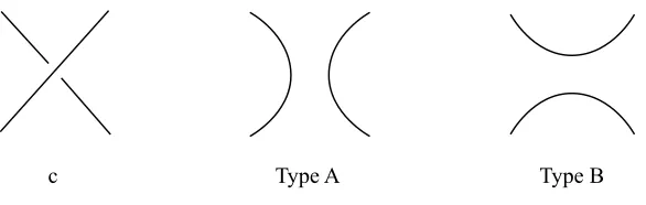
Definition 2.5.6. Let D be an unoriented knot diagram with n crossings. The Kauffman res-olution of a crossing c replaces the crossing with two unlinked bands as in Fig. 2.13.
c Type A Type B
Figure 2.13: Kauffman Resolutions
Armed with the Kauffman resolution, we now want to bring in some combinatorics that will help us relate knot diagrams directly to knot signatures.
Definition 2.5.7. Let D be a reduced, alternating knot diagram. The state sums sA(D) and
sB(D) are the number of components in an all-A or all-B resolution ofD, respectively.
Theorem 2.5.8. Let D be a knot diagram with all positive (negative) crossings. Then the orientation-preserving smoothings are all Kauffman resolutions of type A (B, respectively).
The proof follows immediately from a comparison of Fig. 2.3 and Fig. 2.13: If we orient the crossing c in the latter figure so that it is a positive crossing (arrows pointing upward), the type A resolution would preserve the orientation. Likewise, if c had been negative, the orientation-preserving smoothing would be a Kauffman resolution of type B.
Two points of caution are worth mentioning: First, on an unoriented knot diagram, if the crossing c is opposite to that in Fig. 2.13, the type A and type B resolutions are reversed. Second, by adding an orientation to a knot diagram, a crossing that appears identical to c in Fig. 2.13 while unoriented may become either a positive or a negative crossing.
We can now present Traczyk’s combinatorial formula for computing knot signatures (see [16]) in an equivalent form that is presented in [4].
Theorem 2.5.9. Let Dbe a reduced, alternating diagram representing a knot K. Then
σ(K) =sA(D)−n+(D)−1 = 1 +n−(D)−sB(D)
where sA(D), sB(D) are as in Def. 2.5.7 and n+(D), n−(D) are the number of positive and
Theorem 2.5.9 provides a convenient and efficient way to compute the signature of a knot from the number of Seifert circles we obtain from Seifert’s algorithm without the need to construct the surface or its Seifert matrix. While this formula still requires some effort to use, especially for diagrams with a large number of crossings, it is far less computationally exhaustive than the method of finding knot signatures through the use of matrices.
However, we have yet to show the relationship between a knot’s signature and its unknotting number, for which we must consider how a crossing change affects the signature.
Theorem 2.5.10. LetK+ andK− be two knots with corresponding diagramsD+ andD− that
differ by a single crossing change. Then σ(K+)−σ(K−) = 0 or ±2.
Cromwell [3] provides a proof of Theorem 2.5.10 using an approach that relies on both homology theory and linear algebra related to Seifert surfaces corresponding to either knot.
Corollary 2.5.10.1. Let K be a knot. Then u(K)≥ 12|σ(K)|.
Proof If K is the unknot, then u(K) =σ(K) = 0. Suppose K is a nontrivial knot. Then Theorem 2.5.10 says that each crossing change either leaves the signatureσ(K) unchanged or increases/decreases its value by 2. If every crossing change is made so that it decreases the knot’s signature, it would require exactly 12|σ(K)| crossing changes to reduce σ(K) to zero, showing that K has been unknotted. Therefore, u(K)≥ 1
2|σ(K)|.
It should be noted that equality in Corollary 2.5.10.1 is achieved only when every crossing change reduces the knot’s signature; however, there may be cases in which a crossing change will increase or not affect the knot’s signature. Therefore, the signature only establishes a lower bound for the knot’s unknotting number.
Recall that if Dis a diagram ofK, thenu(D) is an upper bound foru(K) becauseu(K) is the minimum ofu(D) over all diagrams, so even if there is some diagramD0withu(D0)> u(D), the value ofu(D0) would not be the minimum over all diagrams of K.
Together with Corollary 2.5.10.1, this provides a method for determining the unknotting number ofK: First find a lower bound foru(K) by computingσ(K), and then unknot a diagram
3
4
5
6
1
1
2
1
Figure 2.14: Seifert Surfaces Seifert surfaces for the knots 31 (the trefoil), 41 (the
figure-eight), 52, and 61. The left column shows knot diagrams from [13]. The central and right columns
Chapter 3
Unknotting Numbers of Knot
Families
3.1
Conway Notation
Thus far we have referred to knots either by their common names (the unknot, the trefoil, the figure-eight) or by their place in knot tables (31,41,52). Unfortunately, this method does not
always provide the ease and clarity we desire to work efficiently with knots. Therefore, we will introduce a new representation of knots called Conway notation; however, we shall do this in a partial manner, covering only what is needed in this paper. See [9] for a complete introduction to Conway notation.
Conway notation uses tangles as the building blocks of knots, and by combining tangles, we obtain more complicated knots. However, it should be noted that Conway notation cannot describe all knots, and those that it can describe are calledalgebraic knots.
Definition 3.1.1. Let D be a knot diagram. A tangle is a region of D where four arcs meet. The elementary tangles are those with zero or exactly one crossing. See Fig. 3.1.
0 +1 -1
Although the elementary tangles have either zero or one crossings, in general a tangle may have any number of crossings, either all negative or all positive. There are many ways to combine tangles into knots; we will only describe the two we will use.
Definition 3.1.2. Let T and S be two tangles with tand s crossings, respectively.
• The negative of T, denoted −T, is the reflection of T across a diagonal line tangent to the tangle’s boundary on the north-east side.
• The product of T and S, denoted t, s, is the closure of T and S side-by-side.
• The sum ofT and S, denotedt s, is the product of T and −S.
Connecting groups of tangles is called closure, and tangles can be closed in two ways: Both begin by connecting the the outgoing arcs of side-by-side tangles to each other in a way that does not add any crossings. The second step is as follows:
• Denominator closure connects the remaining arcs with arcs on the left- and right-hand sides of the tangles with no additional crossings.
• Numerator closure connects the remaining arcs with arcs above and below the tangle with no additional crossings.
Unless otherwise noted, numerator closure is assumed in Conway notation. See Fig. 3.2.
T
S
T
T
T
S
(a) (b) (c)
Figure 3.2: Tangle Operations(a) the construction of −T from T; (b) the sum ofT andS, denoted t s; (c) the product of T and S, denotedt, s.
Definition 3.1.3. A three-tangle pretzel knot P[p,q,r] is the knot with Conway symbol p,q,r. Definition 3.1.4. A two-bridge knot R[a,b] is the knot with Conway symbol a b.
We are interested in knot families because they often possess enough similarity that we may be able to determine a standard formula for each family that produces some interesting value. For example, under certain circumstances, is it possible to express the unknotting number of the knotP(p, q, r) in terms ofp,q, andr? This idea will be explored further in Section 3.4, but we need an additional measurement to show this.
3.2
The BJ-Unlinking Number
In Def. 2.3.2, the unknotting number of a diagram D was defined as the smallest number of simultaneous crossing changes that would transformDinto a diagram of the unknot. However, would it be possible to find u(D) by performing a sequence of individual crossing changes, rather than making them at the same time?
Definition 3.2.1. Let D be a minimal diagram representing the link L. The BJ-unlinking number uBJ(D) of a diagram D is defined recursively in the following manner [8]:
1. uBJ = 0 if and only if D represents an unlink.
2. Assume the set of diagrams Dk with uBJ(D) ≤k are already defined. A diagram D has
uBJ(D) = k+ 1 if D 6∈ Dk and there exists a crossing v on the diagram D such that
uBJ(Dv0) =k where Dv0 is a minimal diagram representing the same link as diagram Dv
obtained from D by a crossing change at v. Notice that uBJ(D) is well-defined for every
diagram D as D∈ Dn! where n=c(D).
The BJ-unlinking number uBJ(L) of a link L is defined by uBJ(L) = minDuBJ(D) over all
minimal diagrams D representing L.
The BJ-unlinking number, named after J. A. Bernhard and S. Jablan, is defined broadly for links, but since knots are one-component links, it applies equally well to the study of knots. In particular, Def. 3.2.1 gives an algorithmic structure for finding the BJ-unlinking number for a diagramD, making it more easily computable than u(D):
1. Begin with a minimal diagramD with labeled crossingsv1, v2, ..., vn.
2. Perform a single crossing change on the diagramD; without loss of generality, assume the crossingvn is changed, giving the diagramDvn.
3. Reduce the diagramDvn and call this diagramD 0
4. Continue this process, changing a single crossing and then reducing the diagram, until the reduced diagram represents the unknot.
5. Repeat this process for all possible sequences of crossing changes in D; the minimum of these numbers is the BJ-unlinking number ofuBJ(D) of the diagramD.
To move from the BJ-unlinking number of a diagram D to the BJ-unlinking number of a linkL, simply take the minimum of uBJ(D) over all minimal diagramsD representingL.
Since uBJ(L) can be found algorithmically, it is easier to find uBJ(L) thanu(L). However,
are these two numbers necessarily equal?
Conjecture 3.2.2 (Bernhard-Jablan Conjecture). For every link L, u(L) =uBJ(L) [1, 6].
The challenge with conjectures is that they are not theorems, and while no counterexample has shown the Bernhard-Jablan Conjecture to fail, many knot theorists suspect it is false.
Remark 3.2.3. For any link L, even if the Bernhard-Jablan Conjecture does not hold, the BJ-unlinking number is an upper bound for the unlinking number [8]:u(L)≤uBJ(L).
This can easily be shown simply by keeping track of the sequence of crossings changes performed to compute the BJ-unlinking number and then making all the same crossing changes simultaneous in the original diagram. Then, because it’s the unknotting number of a diagram, it is an upper bound for the knot’s unknotting number.
However, at times this process does not yield a small enough upper bound to achieve the lower bound determined from the signature, and at times the signature itself may provide too low a bound to be useful, making it impossible to squeeze out the unknotting number. This idea of a range of possibilities, a gap, motivates the following definition.
Definition 3.2.4. The BJ-unlinking gap of either a diagram D or a link L is as follows:
• δBJ(D) =u(D)−uBJ(D)
• δBJ(L) =uM(L)−uBJ(L)
where uM(L) is the unlinking number ofL over all minimal diagrams.
Remark 3.2.5. Let δ0BJ(D) = minDδBJ(D) where D is a minimal diagram. For alternating
links, we have that δBJ0 (D) =δBJ(D) [8].
3.3
Unknotting the
P
[3,3,2]Pretzel Knot
Jablan and Sazdanovic’s paper [8] defines the BJ-unlinking number and gap and then proves a number of propositions and theorems concerning the calculation of these numbers as well as the unknotting numbers of certain classes of knots. Their paper is motivated by the Nakanashi-Bleiler example (see Fig. 2.8) and its peculiar property that the unknotting number is not realized by a minimal diagram. They further provide many experimental results of the BJ-unlinking gap to illustrate their earlier findings.
In the following section we will discuss their results concerning bridge and pretzel knots, but first we will begin with a motivating example. Explicitly finding the unknotting number of a single knot will allow us to show how the established theory can be used to find a knot’s unknotting number, and furthermore, we will later be able to use our findings to illustrate the proofs of Jablan and Sazdanovic’s theorems in Section 3.4.
We will consider the pretzel knotP[3,3,2]belonging to the familyP[2k+1,2l+1,2m], withk, l, m≥
1. See Fig. 3.3 for the standard diagram of P[3,3,2] and Fig. 3.4 for its possible Seifert surfaces.
Figure 3.3: P(3,3,2) (85 in knot tables) shown as a pretzel knot.
Using results from [13] and the computational powers of [18], we obtain the following Seifert matrixV and the diagonalization ofV +VT, denoted V0 in Fig. 3.5.
-1 0 0 -1 -1 -1
0 1 0 0 0 0
-1 0 -1 -1 -1 -1 0 -1 0 -1 -1 -1 0 -1 0 0 -1 0
0 -1 0 0 -1 -1 V = -1 -1 -6 -1 -1 3 V' =
-2 0 -1 -1 -1 -1 0 2 0 -1 -1 -1 -1 0 -2 -1 -1 -1 -1 -1 -1 -2 -1 -1 -1 -1 -1 -1 -2 -1 -1 -1 -1 -1 -1 -1 V+V =T
Figure 3.5: Seifert Matrix for P[3,3,2] V obtained from [13] and V0 computed using [18].
Diagonal entries of V0 were rounded to the nearest non-zero integer for clarity of presentation.
V0 has one positive entry and five negative entries along the diagonal (see Fig. 3.5), so
σ(P[3,3,2]) = −4. Alternatively, we can use the formulas from Theorem 2.5.9 to compute the signature ofP[3,3,2] without computing the Seifert matrix. See Fig. 3.6 for diagrams of the all-A
and all-B resolutions ofP[3,3,2], necessary for these computations.
+ + + + + + -+ + + + + + -(a) (b)
Figure 3.6: Kauffman Resolutions of P[3,3,2]Diagrams for the all-A (a) and all-B (b)
Kauff-man resolutions. Positive and negative crossings (orientation not shown) have been marked.
Using the observations from Fig. 3.6 thatsA= 3,sB = 5,n+= 6, andn−= 2, we have the
following calculations:
This confirms our earlier calculation of the signature using the Seifert matrix. In particular, we have that u(P[3,3,2])≥
|σ|
2 = 2, since half the signature is a lower bound for the unknotting
number. Recall that because we can only perform a positive number of crossing changes, in cases (such as this one) when the signature of a knot is negative, the negative sign is disregarded while computing the lower bound for the unknotting number.
Finally, observe in Fig. 3.7 that we can unknotP[3,3,2]using only two crossing changes. Since the unknotting number of any diagram is an upper bound for the unknotting number of a knot, we have that u(P[3,3,2]) ≤ 2. Combining this result with the lower bound obtained from the
signature, this proves that the unknotting number ofP[3,3,2] is 2.
Figure 3.7: Unknotting P[3,3,2] The two crossing changes that unknot P[3,3,2] are circled in the first diagram. Moving left-to-right, the strands moved between diagrams are color coded.
3.4
Formulas for Knot Families
Theorem 3.4.1 (Jablan-Sazdanovic). Let Ra,b denote a two-bridge knot or link with the
Con-way symbol a b. Then the following results hold [8]:
1. If a, b are both odd, then for a link R[a,b] = R[2m+1,2n+1], we have uBJ(R[2m+1,2n+1]) = uM(R[2m+1,2n+1]) =u(R[2m+1,2n+1]) =a+2b =m+n+ 1.
2. If ais odd and bis even, then for a knot R[a,b]=R[2m+1,2n], we have uBJ(R[2m+1,2n]) = uM(R[2m+1,2n]) =u(R[2m+1,2n]) =n.
3. Ifa, bare both even, then for a knotR[a,b]=R[2m,2n], we have uBJ(R[2m,2n]) =uM(R[2m,2n]) =
min{m, n}.
Note the unknotting number of R[2m,2n] is an open question for most knots with m, n≥1. Proof The proof of Theorem 3.4.1(1) begins by showing that changingm+ 1 crossings in the first bridge, skipping a crossing between each change, reduces the bridge to a single crossing. Likewise, changing ncrossings in an opposite alternating manner in the second bridge reduces it to a single crossing. However, because these crossings are of the same type, repeated use of R2 Reidemeister moves reduces the diagram to that of a two-component unlink. Sincem+n+ 1 crossing changes unlink a single diagram,m+n+ 1 is an upper bound for the unlinking number of knots in this family. See Fig. 3.8 for an example using the knotR[3,3].
Figure 3.8: Unlinking R[3,3] By Theorem 3.4.1(1), we have that u(R[3,3]) = 3+32 = 3. The
three crossings have been circled.
In the two-bridge diagrams for knots of the type R[a,b] = R[2m+1,2n+1], notice that every
crossing is a crossing between the two components of the link, and every crossing has the same sign. This means the linking numberlk(R[2m+1,2n+1]) is equal tom+n+ 1. The linking number
Combining this result with the upper bound achieved by unknotting a single diagram, we have thatm+n+ 1≤u(R[2m+1,2n+1])≤m+n+ 1, proving our claim.
To prove Theorem 3.4.1(2), we use the signature of the knot rather than the linking number as in part (1), from which we obtain the result. Note that, for two-bridge knots of the form
R[a,b] = R[2m+1,2n], the signature is equal to 2n = b. This can be easily shown by using the
combinatorial formula for computing signatures from Theoren 2.5.9. We begin by orienting the knot so that all crossings are negative and then taking the all-A Kauffman resolution of the diagram. In Fig. 3.9, this is illustrated forR[3,2]and the general caseR[2m+1,n2]. Thus there are
no positive crossings and sA= (2n−1) + 2 = 2n+ 1, so
σ(R[2m+1,n2]) =sA−n+−1 = (2n+ 1)−0−1 = 2n.
Therefore, |σ(R[2m+1,n2])|/2 = |2n|/2 = n is a lower bound for the unknotting number of R[2m+1,n2]. To realize this number, note that changing n crossings in the second bridge transforms the diagram into the unknot, proving this part of the theorem.
-2m
2n-1
2n-1
circles(a)
(b)
Figure 3.9: sAof R[2m+1,2n]In (a), we showR[3,2]can be oriented to have all negative crossings
Theorem 3.4.1(3) requires induction on min{m, n}. Details may be found in [8].
We now turn to a theory from [8] concerning the unknotting number of pretzel knots.
Theorem 3.4.2(Jablan-Sazdanovic). LetP[a,b,c]denote a three-chain pretzel knot with Conway
symbol a, b, c. We have the following results [8]:
1. Ifa, b, care all even, we have a two-component link withuBJ(P[2k,2l,2m]) =uM(P[2k,2l,2m]) = u(P[2k,2l,2m]) =k+l+m+ 1.
2. Ifa, b, care all odd, then fork, m≥1, we haveuBJ(P[2k+1,2l+1,2m+1]) =uM(P[2k+1,2l+1,2m+1]) = l+ minm, k+ 1.
3. Ifa, care odd withbeven, andk, m≥1, we haveuBJ(P[2k+1,2l,2m+1]) =uM(P[2k+1,2l,2m+1]) = u(P[2k+1,2l,2m+1]) =k+m.
Note that u(P[2k+1,2l+1,2m+1]) is an open question for most knots with k, m≥1.
In [8], Jablan and Sazdanovic present additional formulas for other families of three-chain pretzel knots, but these have more complicated formulas and do not in general realize the unknotting numbers of these families. Curious readers should consult the original paper.
Proof We will look at a proof for Theorem 3.4.2(3) only. First, note that for pretzel knots, a cyclic permutation of the parameters produces knots of the same type; therefore, the knot P[3,3,2] from the previous section is a pretzel knot in the family P[2k+1,2l,2m+1], with
k = l = m = 1. From our earlier computations, we know that u(P[3,3,2]) = 2, and by this
theorem,u(P[3,3,2]) = 1 + 1 = 2, so the formula agrees with our findings.
How can we show this in general? First, we must show that the signature is ±2(k+m) so that k+m is a lower bound for the unknotting number; then we must show that this lower bound can be achieved, as we did in our example using P[3,3,2].
We find the signature is the same manner as we did while proving Theorem 3.4.1: Orient a general diagram representingP[2k+1,2l,2m+1], find the number of positive (negative) crossings,
and calculate how many circles in the all-A (or all-B) Kauffman resolutions. As it turns out, regardless of our choice of orientation, the crossings in the 2k+ 1 and 2m+ 1 chains are all positive, while the 2l crossings in the last chain are negative. In Fig. 3.10 (top of next page), we show the general Kauffman resolutions obtained from these oriented diagrams.
We can now directly compute the signature ofP[2k+1,2l,2m+1]:
σ(P(3,3,2)) =sA−n+−1 = 3−(2k+ 2m+ 2)−1 =−2(k+m)
σ(P(3,3,2)) = 1 +n−−sB= 1 + 2l−(2k+ 2l+ 2m+ 1) =−2(k+m)
Type A Type B 2m 2n-1
circles
2k
circles circles
Figure 3.10: Kauffman Resolutions of P[2k+1,2l,2m+1]
Finally, to realize this unknotting number, begin with the standard diagram of the knot
P[2k+1,2l,2m+1]. Without loss of generality, assume k ≥ m. Working with the left-most chain (containing 2k+ 1 crossings), label by 1, ...,2k+ 1 each crossing from top to bottom. Change each crossing labeled with an odd number; if at this point we have made fewer than k+m
crossing changes, make the remaining number of changes in the right-most column (with 2m+ 1 crossings) in a similar fashion as before. Using Reidemeister moves, it is now easy to show this diagram represents the unknot.
However, if 2l > min{2k+ 1,2m+ 1}–as in the Nakanashi-Bleiler example (Fig. 2.8)–this algorithm does not work. In this case, it is necessary to use one of the arcs of the chain with 2l
crossings to increase the shorter of the two remaining chains by two crossings. Then, starting with the first of these two new crossings, changing all odd-numbered crossings in the chain as before. While creating these new crossings, it is important to add them so that they are of the same sign as the other crossings in the chain. With this, our proof is complete.
3.5
Conclusion
This paper has only partially addressed knot theory, and even with everything we have shown about computing the unknotting numbers of certain two-bridge and three-chain pretzel knots, there are many more families for which little or nothing is known in regards to finding their unknotting numbers. There are also more modern and more powerful methods of computing unknotting numbers, such as the signature function and Heegaard’s Knot Floer homology.
References
[1] J. Bernhard.Unknotting numbers and their minimal knot diagrams. J. Knot Theory Ram-ifications, 3, 1 (1994).
[2] J. Collins.Seifert Matrix Computation. http://www.maths.ed.ac.uk/ jcollins/SeifertMatrix/
[3] P. Cromwell. Knots and Links. Cambridge University Press, Cambridge, 2004.
[4] O. Dasbach, A. Lowrence. Turaev Genus, Knot Signature, and the Knot Homology Con-cordance Invariants. Cornell University Library, 2010. arXiv:1002.0898v1 [math.GT]
[5] A. Hatcher.Algebraic Topology. Cambridge University Press, 2002.
[6] S. Jablan.Uknotting number and ∞-unknotting number of a knot. Filomat, 12, 1 (1998).
[7] S. Jablan, R. Sazdanovi´c. LinKnot - Knot Theory by Computer, Series on Knots and Everything Vol. 21, World Scientific, Singapore.
e-print:http://math.ict.edu.rs:8080/webMathematica/LinkSL/cont.htm
[8] S. Jablan, R. Sazdanovi´c.Unlinking Number and Unlinking Gap. Cornell University Library, 2007. arXiv:math/0503270v2 [math.GN]
[9] L. Kauffman.On Knots. Princeton University Press, Princeton, 1987.
[10] L. Kauffman.State Models and the Jones Polynomial. Topology Vol. 26, No. 3, 1987.
[11] L. Kauffman, L. Taylor. Signature of Links, Transactions of the American Mathematical Society Vol. 216, 1976.
[12] C. Livingston.Knot Theory, number 24 of the Carus Mathematical Monographs. Mathe-matical Association of America, Washington, DC, 1993.
[14] J. Munkres.Topology, NJ Prentice Hall, Inc. 2000.
[15] K. Murasugi.On a certain numerical invariant of link types. Trans. Amer. Math. Soc. 117, 1965.
[16] P. Traczyk.A combinatorial formula for the signature of alternating diagrams, Fund. Math. 184, 2004.
[17] J. van Wijk, A. Cohen.Visualization of Seifert Surfaces. IEEE Transactions on Visualiza-tion and Computer Graphics, Vol. 1, No. X, 2006.