Rewriting Variables: the Complexity of Fast
Algebraic Attacks on Stream Ciphers
Philip Hawkes and Gregory G. Rose Qualcomm International, Australia
Level 3, 230 Victoria Road, Gladesville, NSW 2111 Australia {phawkes,ggr}@qualcomm.com
Abstract
Recently proposed algebraic attacks [AK03,CM03] and fast algebraic attacks [A04,C03] have provided the best analyses against some deployed LFSR-based ciphers. The process complexity is exponential in the degree of the equations. Fast algebraic attacks were introduced [C03] as a way of reducing run-time complexity by reducing the degree of the system of equations. Previous reports on fast algebraic attacks [A04,C03] have underestimated the complexity of substituting the keystream into the system of equations, which in some cases dominates the attack. We also show how the Fast Fourier Transform (FFT) [CT65] can be applied to decrease the complexity of the substitution step, although in one case this step still dominates the attack complexity. Finally, we show that all functions of degree d satisfy a common, function-independent linear combination that
may be used in the pre-computation step of the fast algebraic attack and provide an explicit factorization of the corresponding characteristic polynomial. This yields the fastest known method for performing the pre-computation step.
1 Introduction
Many popular stream ciphers are based on linear feedback shift registers (LFSRs) [R91]. Such ciphers include E0 [B01], LILI-128 [SDGM00] and Toyocrypt [MI02]. They
consist of a memory register called the state that is updated (changed) every time a
keystream output is produced, and an additional device, called the nonlinear combiner. The nonlinear combiner computes a keystream output as a function of the current LFSR state.1 The sequence of states produced by an LFSR depends on the initial state of LFSR, which is always presumed to be secret. Since recovering this initial state allows prediction of unknown keystream, we follow the convention of [C03] and call it K as if it
was actually the key. Most practical stream ciphers initialize this state from the real key and a nonce. The advantages of LFSRs are many. LFSRs can be constructed very efficiently in hardware and some recent designs are also very efficient in software. LFSRs can be chosen such that the produced sequence has a high period and good statistical properties.
While there are many approaches to the cryptanalysis of LFSR-based stream ciphers, this paper is concerned primarily with the recently proposed algebraic attacks [AK03,CM03] and fast algebraic attacks [A04,C03]. Such attacks have provided the best analyses against some theoretical and deployed ciphers.
1 Some LFSR-based stream ciphers have a non-linear filter that maintains some bits of memory, but
An algebraic attack consists of three steps. The first step is to find a system of algebraic equations that relate the bits of the initial state K and bits of the keystream Z = {zt}.
Some methods [AK03,CM03] have been proposed for finding “localized” equations (where the keystream bits are in a small range zt,…,zt+θ). This first step is a
pre-computation: the attacker must compute these equations before attacking a key-stream. Furthermore, the computation need only be performed once, and the attacker can use the same equations for attacking multiple key-streams. The second and third steps are performed after the attacker has observed some keystream. In the second step, the observed keystream bits are substituted into the algebraic equations (from the first step) to obtain a system of algebraic equations in the bits of K. The third step is to solve these
algebraic equations to determine K. This will be possible if the equations are of low
degree in the bits of K, and a sufficient number of equations can be obtained from the
observed keystream.
The process complexity of the third step is exponential in the degree of the equations. Fast algebraic attacks were introduced by Courtois at Crypto 2003 [C03] as a way of reducing run-time complexity by reducing the degree of the system of equations. This method requires an additional pre-computation step; this step determines a linear combination of equations in the initial system that cancels out terms of high degree (provided the algebraic equations are of a special form). This yields a second system of equations relating K and the keystream Z that contains only terms of low degree. In the
second step, the appropriate keystream values are now substituted into this second system to obtain a new system of algebraic equations in the bits of K. Solving the new system (in
the third step) is easier than solving the old system because the new system contains only terms of low degree.
Courtois [C03] proposes using a method based on the Berlekamp-Massey algorithm [M69] for determining the linear combination obtained in the additional pre-computation
step. The normal Berlekamp-Massey algorithm has a complexity of D2, while an
asymptotically-fast implementation has a complexity of C⋅ D (log D) for some large
constant C. It is unclear which method would be best for the size of D considered in these
attacks. Armknecht [A04] provides a method for improving the complexity when the cipher consists of multiple LFSRs.
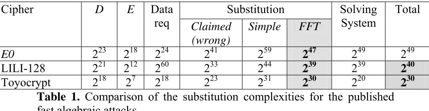
Contributions of this paper. The first contribution is to note that previous reports on fast algebraic attacks (such as [A04,C03]) appear to have underestimated the complexity of substituting the keystream into the second system of equations.2 The complexity was
originally underestimated as only O(DE) [C03], where D is the size of the linear
combination and E is the size of the second system of equations. Table 1 lists the values
of O(DE)for previously published attacks from [A04,C03]. However, simple substitution
would require a complexity of O(DE2) (see Section 2.3), and no other method was
suggested for reducing the complexity. It is true that E bitwise operations of the
substitution can be performed in parallel, reducing the time complexity to O(DE), but in
cases where E is large, the process complexity should still be considered O(DE2) in the
2 We are aware (via private communication) of other proposed algebraic attacks in which the substitution
absence of specialized hardware. In many cases DE2 actuallyexceeds the complexity of
solving the system of equations, as shown in Table 1.
The second contribution of this paper is to show how the Fast Fourier Transform (FFT) [CT65] can be applied to decrease the complexity of the substitution step from the naïve
DE2/2 to 2EDlog2D. The resulting complexities of the FFT approach are also listed in
Table 1.
Substitution
Cipher D E Data
req Claimed
(wrong)
Simple FFT
Solving System
Total
E0 223 218 224 241 259 247 249 249
LILI-128 221 212 260 233 244 239 239 240
Toyocrypt 218 27 218 223 231 230 220 230
Table 1. Comparison of the substitution complexities for the published fast algebraic attacks.
The final contribution of this paper is to provide an efficient method for determining the linear combination obtained in the additional pre-computation step of the fast algebraic
attack. First we show that all functions of degree d satisfy a common
function-independent linear combination of length D= ∑i=0..d Cndthat is defined exclusively by the
LFSR. Then we provide a direct method for computing this linear combination (based on the work of Key [K76]). This method requires c ⋅ D (log D)2 operations, where c is a
small constant. This is a significant improvement on the complexities of previous methods.
Courtois [C03]: based
on Berlekamp-Massey Armknecht [A04]
Cipher D
C⋅ D (log D) D2 Parallel Method
Direct Computation (this paper)
D (log D)2
E0 223 C⋅ 228 246 243 232
LILI-128 221 C ⋅ 226 242 - 230
Toyocrypt 218 C ⋅ 223 236 - 226
Table 2. The complexities of the pre-computation step for published attacks, where C represents a large constant.
This paper is organized as follows: in Section 2 we describe fast algebraic attacks. In Section 3 we discuss the complexity of substitution step for fast algebraic attacks. Section 4 reviews some useful properties of FFTs. Section 5 describes how the Fast Fourier Transform can be applied to speed up the substitution step. Section 6 contains our observations about the linear combination used in the fast algebraic attack. Section 7 concludes the paper.
2 Fast Algebraic Attacks
The length of the LFSR is n-bits; that is the internal state of the LFSR is Kt∈GF(2)n. A
state Kt+1is derived from the previous state Ktby applying an (invertible) linear mapping
matrix over GF(2), which is called the state update matrix. Notice that we can write Kt
=Lt(K). Each keystream bit is generated by first updating the LFSR state (by applying L)
and then applying a Boolean function to the bits of the LFSR state. For the purposes of this paper, everything about the cipher is presumed to be known to the attacker, except the initial state of the LFSR and any subsequent state derived from it.
Linearization: Recall that the first two steps of the attack result in a system of nonlinear algebraic equations in a small number of unknown variables (these variables being the bits of the initial state). The most successful algebraic attacks (to date), have been based on linearization. The basis of this technique is to “linearize” a system of nonlinear algebraic equations by assigning a new unknown variable to each monomial term that appears in the system. The same monomial term appearing in distinct equations is assigned the same new unknown variable. The system of equations then changes from a system of non-linear equations (with few unknown variables) into a system of linear equations (with a large number of unknown variables). If the number of linear equations exceeds the number of new unknown variables, then an attacker can solve the system to obtain the new unknown variables of the linear system (which will in turn reveal the unknown variables of the non-linear system). The advantage of linearization is that the attacker can use the large body of knowledge about the solution of linear systems.
2.1 The Monomial State
This section introduces some notation that is useful for describing linearization. For a given value of the state Kt and for a given degree d, we shall let Md(t) (the monomial state) denote the GF(2) column vector with each component being a corresponding
monomial of degree d or less. The number of such monomials is D =∑i=0..d Cni ~ Cnd, so Md(t) contains D components. The initial monomial state Md corresponds to the initiate
state K.
Example 1. If n=4 (that is, Kt = k3 k2 k1 k0) and d=2, then there are D=11 monomials of
degree ≤ 2:
Md(t) = (m0, m1, m2, m3, m4, m5, m6, m7, m8, m9, m10)T
= (1, k0, k1, k2 , k3, k0 k1, k0 k2, k0 k3, k1 k2, k1 k3, k2 k3)T
where the letter “T” denotes the transpose of the matrix to make a column vector. If Kt
=0111, then the values of the monomials are:
Md(t) = (1,k0 =1, k1=1, k2 =1, k3=0, k0 k1=1, k0 k2=1, k0 k3=0, k1 k2=1, k1 k3=0, k2 k3=0) T
= (1,1,1,1,0,1,1,0,1,0,0) T
Note that the ordering of the monomials is arbitrary; for consistency we will enumerate
using lower subscripts first, as shown.
Example 2. Consider a Boolean function of the state such as the function f(K) = k2 + k1k3
(using the LFSR state from Example 1). This function can be expressed as
f(Kt) = k2 + k1 k3
= 0×1 +0×k0 + 0× k1 +1×k2 + 0×k3 + 0×k0 k1
+ 0×k0 k2 +0×k0 k3 + 0× k1 k2 + 1× k1 k3 +0×k2 k3
= (0,0,0,1,0,0,0,0,0,1,0) ⋅Md(t) = f⋅Md(t). (1)
where the addition and multiplication operations are performed in GF(2).3 We have now
expressed f(Kt)as the product of Md(t) with a row vector f = (0,0,0,1,0,0,0,0,0,1,0) that
selects the values of the specific monomials required to evaluate the function f. Note that the row vector f depends only on the function f(), and is independent of the LFSR feedback polynomial, the value of the initial state, and the index t.
We know the mapping from one LFSR state to the next LFSR state. It is also possible to determine the mapping from one monomial state to the next monomial state.
Example 3. Consider a 4-bit LFSR as in Example 1 with monomial state
Md(t) = (1, k0, k1, k2, k3, k0 k1, k0 k2, k0 k3, k1 k2, k1 k3, k2 k3)T
If the LFSR has is of the form st+4 = st+1 + st, then the next state Kt+1 has a corresponding
next monomial state Md(t+1)= (m’0, m’1, m’2, m’3, m’4, m’5, m’6, m’7, m’8, m’9, m’10)T
which is related to the original monomial state as follows (only some relationships have been shown in order to save space):
m'0 = 1 = 1 = m0 = (1,0,0,0,0,0,0,0,0,0,0) ⋅ Md(t),
m’1 = k’0 = k1 = m2 = (0,0,1,0,0,0,0,0,0,0,0) ⋅ Md(t), m’4 = k’3 = k0 + k1 = m1 + m2 = (0,1,1,0,0,0,0,0,0,0,0) ⋅ Md(t), m’10 = k’2 k’3 = k3(k0 + k1) = m7 +m9 = (0,0,0,0,0,0,0,1,0,1,0) ⋅ Md(t).
Each component of the next monomial state is a linear function of the original monomial state. These linear functions for m'0, …, m'D-1 can be combined into a matrix Rd (the
“rewriting matrix”) such that Md(t+1) = Rd ⋅ Md(t) . This matrix depends only of the
LFSR and the degree d.
This example generalizes: for every LFSR and degree d there is a “monomial state
rewritingmatrix” Rdsuch that Md(t+1) = Rd ⋅ Md(t). Moreover, for every t, the monomial
state after t clocks of the LFSR can be expressed as a GF(2) matrix operation
Md(t) = Rdt ⋅ Md, (2)
where Md is the initial monomial state. Combining equations (1) and (2), we get another
expression for f(Kt):
f(Kt) =f ⋅ (Rdt ⋅ Md) = (f ⋅Rdt) ⋅ Md = ft ⋅ Md , (3)
where: ft =def (f ⋅Rdt)depends solely on the function f , the monomial state update matrix Rd and the number of clocks t (all of which are known to the attacker); and Md is the
unknown initial state.
2.2 Algebraic Attacks
We always assume that the monomial state is unknown; it is the goal of algebraic attacks to determine the initial monomial state Md (and thereby determine the initial LFSR state).
The first step in an algebraic attack is to find a Boolean function h such that the equation
h(Kt, zt . . . , zt+θ) = 0 (4)
is true for all clocks (or indices) t. The degree of h with respect to the bits of Kt we shall
denote by d. Various methods have been proposed for finding such equations (see
[AK03,CM03]). These equations typically have small values for θ. For simplicity we
shall hereafter combine the keystream bit values zt . . . , zt+θ into a keystream vectorzt.
For the linearization approach, it is convenient to obtain an expression for h(Kt, zt) in
terms of the keystream bits and bits of the initial monomial state Md. Based on equation
(3) we can re-write
h(Kt,zt) =h(zt) ⋅ (Rdt ⋅ Md) = (h(zt) ⋅Rdt) ⋅ Md = ht(zt)⋅ Md
where the vector ht(zt) =def (h(zt) ⋅Rdt) has components that depend on (a) the function h; (b) the monomial state rewriting matrix Rd associated with the monomials of degree of
degree d or less; (c) the number of clocks t; and (d) the small keystream vector zt.
Equation (4) is then transformed to:
ht(zt) ⋅ Md = 0 (5)
The second step of an algebraic attack is to evaluate many vectors ht(zt), 1 ≤ t ≤ D by
substituting observed keystream vector zt. Each of the evaluated vectors ht(zt) provides
the attacker with a linear equation in the D unknown bits of the initial monomial state Md.
Since there are D unknowns, around D linear equations will be required to obtain a
solvable system. An initial choice of D equations may contain linearly dependent
equations, so more than D equations may be required in order to get a completely
solvable system. It is thought that not many more than D equations will be required in
practice (see remark at the end of section 5.1 of [C03]), so we will assume D equations
are sufficient.
The third step recovers Md by solving the resulting system. The system can be solved by
Gaussian elimination or more efficient methods [S69]. The complexity of solving such a system of equations is estimated to be O(Dω) where ω (the Gaussian coefficient?) is
estimated to be ω = 2.7. In general, D will be about Cnd = O(nd). This means the
complexities of an algebraic attack are as follows:
• The complexity of finding the equation h(Kt,zt) depends on many factors and is
beyond the scope of this paper.
• The amount of keystream required for the second step (the data complexity) is
O(D)=O(nd).
• The complexity of the second step (substituting the keystream) is O(D2) = O(n2d),
assuming that the functions h(Kt,zt) are relatively simple functions of the
keystream; and
Note 1. The complexity is exponential in the degree d. Hence, the low degree d is
required for an efficient attack. Therefore, an attacker using an algebraic attack will
always try to find a system of low degree equations.
2.3 Fast Algebraic Attacks
Courtois [C03] proposed “fast algebraic attacks”, as a method for decreasing the degree of a given system of equations. For fast algebraic attacks, we presume that the function H
can be written in the form
h(Kt, zt . . . , zt+θ) = f(Kt) + g(Kt,zt) = 0, (6)
where f is of degree d in the bits of Kt, and g is of degree e < d in the bits of Kt. Since the
functions f and g are of two distinct degrees, it is simplest if we consider them as
depending on distinct monomial states Md and Me, with corresponding monomial state
rewriting matrices Rd and Re. The number of monomials of degree d or less is D =∑i=0..d Cni ~ Cnd, and the number of monomials of degree d or less is E =∑i=0..eCni ~ Cne.
A fast algebraic attack obtains an advantage over the normal algebraic attacks by
including an additional pre-computation step in which the attacker determines linear
combinations of equation (6) that will cancel out the high-degree monomials of degree {e+1, e+2,…,d} that occur in f(Kt), but not in g(Kt zt).
First note that equation (3) allows F(Kt) and G(Kt zt) to be re-written as f(Kt) = ft ⋅ Md ,
and g(Kt zt) =gt(zt) ⋅ Me , where ft = (f ⋅Rdt) and gt(zt) =(g (zt) ⋅Ret). Equation (6) is then
transformed to:
ft ⋅ M d + gt(zt) ⋅ Me = 0. (7)
In the fast algebraic attack pre-computation step, the attacker finds (D+1) coefficients b0,…, bD∈ {0, 1} such that
∑i=0..Dbi ft+i= 0, ∀t. (8)
Equations (7) and (8) can be combined:
∑i=0..Dbi(ft+i ⋅ M d + gt+i(zt+i) ⋅ Me ) = (∑i=0..Dbi gt+i(zt+i)) ⋅ Me
Thus, we obtain a linear expression in Me
g’t(z’t) ⋅ Me = 0, where (9)
g’t(z’t) =∑i=0..Dbigt+i(zt+i). (10)
The second step of a fast algebraic attack is to evaluate many vectors g’t(z’t), by
substituting observed keystream vectors zt in equation (10). Each of the evaluated vectors g’t(z’t) provides the attacker with a linear equation in the E unknown bits of the initial
monomial state Me. Equation (9) involves fewer unknowns than the initial equation (6)
degree d, so fewer equations (9) are required in order to solve for the unknowns.
Reducing the number of unknowns and equations significantly improves the third step of the attack as solving the system of E equations (9) takes significantly less time than solving the system of D equations of (5). Since there are only E unknowns in Me, the
Courtois [C03] and Armknecht [A04] have proposed efficient methods for finding the coefficients of equation (8). The details are not relevant to this paper, but the complexities are provided in Table 2 for the purposes of comparison with the method proposed in Section 6 of this paper.
At this point, it is worth noting that evaluating g’t(z’t) (for each equation (9)) requires
substituting the bits from the D keystream vectors {zt+i, 0≤i≤D}. Obtaining E equations
(9) can be achieved using the set of keystream vectors {zt+i, 0 ≤i≤D, 1 ≤t≤E} = {zt+i, 1 ≤ t ≤D+E}.These keystream vectors can be obtained from the keystream bits zt+i, 1 ≤ t ≤ D+E+θ; so the attack can be performed using as few as (D+E+θ)= O(D) keystream bits.
3 Substitution Complexity of Fast Algebraic attacks
Normal algebraic attacks and fast algebraic attacks differ in the complexity of substituting the keystream into the equations in step two. The function h(zt) is a function
of a small number of keystream bits zt+i, 0 ≤ i≤θ; but the function g’t(z’t) is a function
of a large number of keystream bits zt+i, 0 ≤ t ≤ D+θ. This must be taken into account
when determining the substitution complexity. The attacks in [A04,C03] underestimated the substitution complexity. The root cause appears to be a misunderstanding (discussed in the introduction).
The simple approach to substituting the keystream is to compute the values of gt(zt) and
then substitute these values into the equations (10) individually.4 Computing a single component of (g’t(z’t) = ∑i=0..Dbi gt(zt)) for a single equation will require complexity D/2,
since (on average) half of the coefficients bi are expected to be zero. There are E terms,
so the complexity of substituting the keystream into a single equation (10) is E× (D/2) = ED/2. However, E equations are required in order to solve the system, and so the total
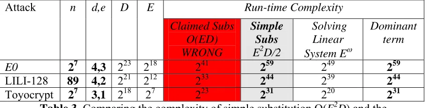
cost of simple substitution will be E× (ED/2) = E2D/2. Table 3 lists the complexity of
simple substitution for the fast algebraic attacks in the literature. Note that the simple substitution significantly exceeds the complexity of solving the linear system of equations in these cases.
Run-time Complexity
Attack n d,e D E
Claimed Subs O(ED) WRONG
Simple Subs E2D/2
Solving Linear System Eω
Dominant term
E0 27 4,3 223 218 241 259 249 259
LILI-128 89 4,2 221 212 233 244 239 244
Toyocrypt 27 3,1 218 27 223 231 220 231
Table 3. Comparing the complexity of simple substitution O(E2D) and the
claimed complexity of substitution O(ED).
4 We ignore the cost of computing
gt(zt) as this cost is independent of the cost of determining g’t(z’t) from
4 The Discrete Fourier Transform
Suppose f(t) is a Boolean function evaluated at P values 1 ≤ t ≤ P. In our case, we are
interested in the functions f(Kt) of the LFSR state Kt. We want to look at a discrete spectral analysis of h.
Real Spectral Analysis: First, we’ll consider a quick tangential topic. A common tool in analyzing a real-valued function f(x) (such as a sound wave) evaluated on a domain x∈
[0,P] is to represents the function f as a sum of simple periodic functions (cosine and sine
curves) where the function f is specified by the amplitudes of these periodic functions.
That is, we represent f as a sum of cosine and sine curves
f(x) = A0+ ∑φ=1..∞ Aφcos( (2πφ/p) ⋅ x) + ∑φ=1..∞ Bφsin( (2πφ/p)⋅ x ) .
with amplitudesAφand Bφ assigned for each frequencyφ. The sequences {Aφ} and {Bφ}
are the Fourier series for f, and evaluating the amplitudes is called a spectral analysis.
Discrete Spectral Analysis: To perform a spectral analysis of the discrete function f(t)
we use a similar idea to represent f(t) using simple periodic functions defined as follows.
Let λ be a value of order P in a field F that (a) contains GF(2) as a subfield and (b) has elements of order P. For example, we could use the complex field, then we would use λ = e2π/P. Alternatively, we could use a Galois Field whose order is divisible by P and then
choose a field element of order P as our value λ. The simple periodic functions that we
use to represent f(t) are the P functions Λφ(t) = λφ⋅t, 0 ≤ φ ≤ (P-1); these functions are
analogous to the sine and cosine curves.
A discrete spectral analysis determines values in the chosen field F (e.g. complex field or Galois field) that correspond to “amplitudes” Fφ∈F. These amplitudes are to be assigned to the P periodic functions Λφ(t) so that
f(t) = ∑φ=0..(P-1) Fφ⋅Λφ(t). (11)
In this way, f(t) is represented as the sum of p periodic functions Λφ(t), 0 ≤ φ ≤ (P-1). It is
well known that the sequence {Fφ} can be computed directly fromthe sequence {f(t)} as:
Fφ= ∑t=1..Pf(t)/pΛφ(-t). (12)
This calculation of {Fφ} from {f(t)} as in (12) is called the Discrete Fourier Transform
(DFT), while the calculation of {f(t)} from {Fφ} is the Inverse DFT.
Properties: There are properties of the DFT that are relevant to this paper:
Linearity: If c(t) = αa(t)+βb(t)∀t, then Cφ=αAφ + βBφ ∀φ.
The convolution of a and b of period p is another function c of period p with c(t) = ∑i=1..P a(t)b( i-t(mod P) ),∀t. It is common to write c = a * b.
Convolution Property: If c = a * b then Cφ =Aφ Bφ ∀φ.
Fast Fourier Transform: The most efficient method for computing the DFT, known as the Fast Fourier Transform (FFT) [CT65], requires a total of Plog2P operations. The
convolution takes P operations. There is also a Inverse FFT that takes the same amount of
5 Applying the FFT to the Substitution Step
The inefficiency of the naïve substitution (in the second step) is indicated by two things:
• The equations (10) often re-use the same values of gt(zt) when computing g’t(z’t).
• The equations (10) all use the same linear combination;
This is the type of computation for which the FFT can offer significant advantages. Suppose the attacker observes the sufficient amount of keystream, and evaluates the coefficients of each of the vectors gt(zt) in equation (7) for 1 ≤ t ≤ D+E. The attacker
wants a fast way to determine the E vectors g’t(z’t) = ∑i=0..Dbi gt+i(zt+i), 1 ≤ t ≤ E, (see
equation (10)) from the (D+E) vectors gt(zt).
Notation: We define a function sequence g(t) = gt(zt), 1 ≤ t≤D+E, with P = D+E. We
require a new discrete function βon the domain1≤ t≤P; defined with β(t) = 0, 1 ≤ t≤ E-1, and β(t) = bp-t, E≤ t≤p. The coefficients b0, b1, …, bD appear in the reverse order
at the end of the sequence {β(t)}, with the remainder of the sequence filled with zeroes.
We chose this function because, on the domain 1 ≤ t ≤ E, the convolution (g*β) has
special properties. First,
(g*β) (t) = ∑i=1..pβ (i) g(t-i (mod P))
= ∑i =1..E-1 β (i) g(t-i (mod P)) + ∑i=E..pβ (i) g(t-i (mod P))
= ∑i=E..p b(p-i) g(t-i (mod P))
Now substitute j = (P- i), so the sum is performed over the domain 0 ≤ j≤D. For these
values of j, we notice that t-i ≡t- (P-j) ≡t+j (mod P),and thus,
g(t-i (mod P)) = g(t+j) = gt+j (zt+j ).
⇒ (g(z)*β) (t) = ∑j=0..D bj gt+j (zt+j ) = g’t(z’t)
This is, the convolution contains the values of g’t(z’t)! Now, if we can find a fast way for
computing the convolution (g*β)(t), we may have a faster method for computing g’t(z’t)
from the values of gt(zt). This is where the Fast Fourier transform is useful.
For simplicity, denote the DFTs corresponding to g(t) and β(t) by Gφ and Bφ respectively. We are going to compute g’t(z’t) by first computing G and B. We then
exploit the convolution property which states that if we compute the values of Qφ = Gφ
Bφ and then apply the inverse DFT to Q, then the resulting function q is the convolution
of g(z) and β, that is q(t) = (g*β)(t). The first E vectors q(t), 1 ≤ t≤E, will correspond
to the vectors g’t(z’t); that is g’t(z’t) = q(t), 1 ≤ t≤E.
This may seems like a strange way to compute g’t(z’t), but it is very efficient when the
FFT is applied:
• The DFT B of β can be pre-computed (since it is always the same): the FFT
requires (D+E) log2 (D+E) ≈D log2D complexity.
• The DFT G of gt(zt)is computed bythe FFT in time ED log2D, since each of the E components must be computed individually.
• Now the DFTs G and B have been computed, Q can be computed from G and B
• Finally, q is obtained from Q by applying the Inverse FFT; this will take time ED
log2D.
• The appropriate vectors g’t(z’t), 1 ≤ t≤E, are obtained directly from q, 1 ≤ t≤E.
The total complexity of computing the vectors g’t(z’t), 1 ≤ t≤E, from the evaluations of
the vectors gt(zt), 1 ≤ t≤ (D+E) is:
ED log2D + (D+E)E + ED log2D≈ 2ED log2D.
The improvement of this method over the naïve substitution is a factor of
E2 D/2 ÷ (2ED log2D)) = E / 4 log2D
So the improvement depends on the size of E relative to 4log2D.
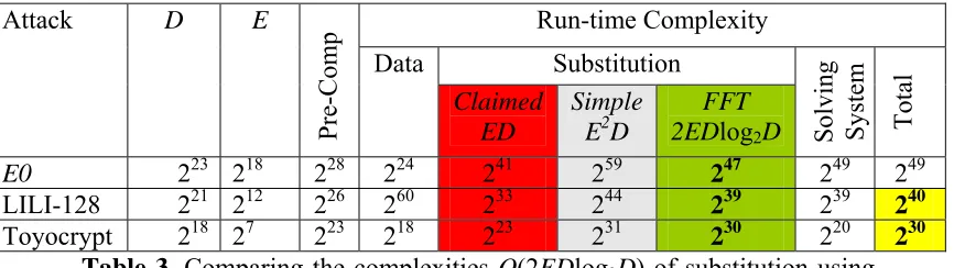
Table 3 shows the complexities of the FFT method for substitution for the current fast algebraic attacks in literature. In the case of E0, the improvement has been significant,
and the substitution step no-longer dominates the run-time complexity. The improvement is less noticeable in the substitutions required for LILI-128 and Toyocrypt. The substitution step still comprises a significant portion of the complexity for these attacks.
Run-time Complexity Substitution
Attack D E
Pre-Comp
Data
Claimed ED
Simple E2D
FFT
2EDlog2D Solving System Total
E0 223 218 228 224 241 259 247 249 249
LILI-128 221 212 226 260 233 244 239 239 240
Toyocrypt 218 27 223 218 223 231
230 220 230
Table 3. Comparing the complexities O(2EDlog2D) of substitution using
the FFT method against the complexities of simple substitution O(E2D/2)
and the claimed complexity of substitution O(ED).
6 Improving the Pre-Computation Step
A Common Linear Combination: It is common knowledge that a square matrix satisfies its characteristic polynomial. That is, if p(x) = ∑i=0..Dpi xi is the characteristic
polynomial of Rd, then
p(Rd) = ∑i=0..D piRdi = 0, (13)
where 0 represents the all-zero matrix. Thus, if the coefficients b0,…, bD of (8) are
assigned the values of the coefficients p0,…, pD of the characteristic polynomial of Rd,
then (∑i=0..Dbi ft+i) = ∑i=0..D(pi ⋅f Rdt+i) = f ⋅ Rdt ⋅ (∑i=0..Dpi Rdi) = f ⋅ Rdt ⋅ 0 = 0. So a
logical choice for the coefficients b0,…, bD of (8) is the values the coefficients p0,…, pD
of the characteristic polynomial of Rd!
Note 2.The characteristic polynomial of Rd depends on the LFSR and the degree d, and is
otherwise independent of the function f. This means that for all functions of degree d, the
coefficients p0,…, pD (of the characteristic polynomial of Rd) can be substituted into the
Direct Computation of the Linear Combination: Suppose an LFSR state Kt of length n
is updated according to state update matrix L, and the characteristic polynomial of L is
primitive.5 The following theorem, while not explicitly stated by Key [K76], is a fairly
obvious consequence of Key’s ideas. We use the notation w(φ) to denote the Hamming
weight of φ (that is, the number of 1’s in the radix-2 representation of the integer φ).
Theorem 1. (Largely due to Key [K76]) A Boolean function f(t)= f(Kt) of degree d can be
expressed as
f(t) = ∑φ: w(φ)≤ d Fφ⋅Λφ(t) = ∑φ: w(φ)≤ dFφ ⋅ (λφ)t (14)
where φ is an n-bit integer, and λ∈GF(2n) is a root of the characteristic polynomial of the
LFSR state update matrix L. Moreover, the polynomial pd(x) = ∏φ: w(φ)≤ d (x – λφ), is
always a characteristic polynomial of f(t).This polynomial is of degree D=∑i=0..dCni .
In other words, the characteristic polynomial of Rd is pd(x) = ∏φ: w(φ)≤ d (x – λφ). Note that
there are D values φ with w(φ)≤ d, so the corresponding linear combination is the
expected length for the sequence {f(t)}.
The authors are not aware of the best complexity of expanding pd(x). As a first upper
bound, consider multiplying pairs of factors to obtain factors of degree 2, then multiply pairs of factors of degree 2 to get factors of degree 4, and so forth. The FFT can be applied to speed up the multiplication. At the j-th step, (starting at j=1) the factors are of
degree T=2j-1. To multiply two factors a(x)= ∑i=0..T aixi and b(x)= ∑i=0..Tbixi,first define
two functions α(i) and β(i) on the domain [0,2T+1], with α(i) = ai, and β(i) = bi, for 0≤i≤T+1, α(i) = 0, and β(i) = 0, for T+2≤i≤2T+1.
The convolution χ(i) = (α * β)(i) contains the coefficients of the c(x) = a(x) × b(x). We
know that the complexity of the convolution is 2⋅ (2T)⋅ log2(2T). Since there will be D/2T
multiplications performed at each step (that is, for each j), the total complexity of this
approach is:
∑j=1..logD (D/2i) ⋅2⋅ 2j⋅log 2j) = 2 ⋅∑j=1..logDD⋅ j= 2D⋅ ∑j=1..logDj
= 2D⋅ (log D⋅ (log D -1) / 2 ) ≈ D (log D)2.
In Table 2, the complexity of this method is compared against the previous methods.
7 Conclusion
We have shown that some published “fast algebraic attacks” on stream ciphers underestimate the process complexity of one of the steps, and we provide correct complexity estimates for these cases. We then show an improved method, using Fast Fourier Transforms, for substituting keystream bits into the system of equations needing to be solved. We also made some observations about the linear combination used in the pre-computation step of the fast algebraic attack. In particular, we found the fastest
5 This approach can be extended to cases where the characteristic polynomial is not primitive; for example,
known method for performing the pre-computation. The fast algebraic attack remains an extremely powerful technique for analyzing LFSR-based stream ciphers.
References
[A04] F. Armknecht: Improving Fast Algebraic Attacks, to be presented at FSE2004
Fast Software Encryption Workshop, Delhi, India, February 5-7, 2004.
[AK03] F. Armknecht and M. Krause: Algebraic Attacks on Combiners with
Memory, proceedings of Crypto2003, Lecture Notes in Computer Science, vol.
2729, pp. 162-176, Springer 2003.
[B01] Bluetooth CIG, Specification of the Bluetooth system, Version 1.1, February 22,
2001. Available from www.bluetooth.com.
[CT65] Cooley, J. W. and Tukey, J. W., 1965, An algorithm for the machine calculation
of complex Fourier series, Mathematics of Computation, 19, 90, pp. 297-301,
1990.
[C03] N. Courtois: Fast Algebraic Attacks on Stream Ciphers with Linear Feedback,
Crypto2003, Lecture Notes in Computer Science, vol. 2729, pp. 177-194, Springer 2003.
[CM03] N. Courtois and W. Meier: Algebraic Attacks on Stream Ciphers with
Linear Feedback, EUROCRYPT 2003, Warsaw, Poland, Lecture Notes in
Computer Science, vol. 2656, pp. 345-359, Springer, 2003.
[K76] E. Key: An Analysis of the Structure and Complexity of Nonlinear Binary
Sequence Generators, IEEE Transactions on Information Theory, vol. IT-22, No.
6, November 1976.
[M69] J. Massey: Shift Register synthesis and BCH decoding, IEE Transactions on
Information Theory, IT-15 (1969), pp. 122-127.
[MI02] M. Mihaljević and H. Imai: Cryptanalysis of Toyocrypt-HS1 stream cipher,
IEICE Transactions on Fundamentals, vol E85-A, pp. 66-73, January 2002.
Available at www.csl.sony.co.jp/ATL/papers/IEICEjan02.pdf.
[R91] R. Rueppel: Stream Ciphers; Contemporary Cryptology: The Science of
Information Integrity. G. Simmons ed., IEEE Press, New York, 1991.
[SDGM00] L. Simpson, E. Dawson, J. Golic and W. Millan: LILI Keystream
Generator; Selected Areas in Cryptography SAC’2000, Lecture Notes in
Computer Science, vol. 1807, Springer, pp. 392-407.
[S69] V. Strassen: Gaussian Elimination is Not Optimal; Numerische Mathematik, vol.