Frequency comb based time transfer over a 159 km long installed fiber network

M. Lessing,1, 2 _{H. S. Margolis,}1_{C. T. A. Brown,}2_{and G. Marra}1,a)

1)

National Physical Laboratory, Hampton Road, Teddington, Middlesex, TW11 0LW, UK

2)_{SUPA, School of Physics and Astronomy, University of St Andrews, St Andrews, Fife, KY16 9SS,}

UK

(Dated: 12 May 2017)

We demonstrate a frequency comb-based time transfer technique on a 159 km long installed fiber link. Timing information is superimposed onto the optical pulse train of an ITU-channel-filtered mode-locked laser using an intensity modulation scheme. The environmentally induced optical path length fluctuations are compensated using a round-trip phase noise cancellation technique. When the fiber link is stabilized a time deviation of 300 fs at 5 s and an accuracy at the 100 ps level is achieved.

PACS numbers: 06

Driven by improvements in the performance of opti-cal atomic clocks, which can now achieve accuracies and stabilities at the 10−18 _level1–3_{, much research has been}

undertaken in the field of frequency transfer via fiber net-works to overcome the limitations of satellite-based tech-niques. It has been shown that the performance of fiber-based optical frequency transfer techniques is suitable for the comparison of state-of-the-art optical clocks on a con-tinental scale4–6_{. Fiber-based time transfer techniques}

have also been shown to offer superior performance com-pared to their satellite-based counterparts. Accuracies of tens of ps have been reported for fiber lengths of hundreds of km7,8 _{which is significantly better than that offered}

by routinely-used satellite-based two-way time transfer techniques (accuracy at the 1 ns level9_{). These}

fiber-based techniques could therefore be beneficial for clock comparisons for the computation of International Atomic Time. Several different fiber-based time transfer tech-niques have been investigated7,8,10–14_.

While there has been a demonstration of two-way time transfer over a 12 km free-space distance with fs level time deviation using optical frequency combs15,16_{, all time}

transfer methods over longer fiber networks to date have been carried out using amplitude-modulated continuous wave (CW) lasers. In previous work, we have demon-strated microwave and optical frequency transfer on a 7 km long fiber link at a level better than 1×10−17 _by

propagation of a 30 nm-wide optical frequency comb17. Here, we demonstrate time transfer over a 159 km long in-stalled fiber network using an ITU-channel-filtered mode-locked laser (MLL). This opens the way for transferring microwave frequencies, optical frequencies and time si-multaneously via fiber networks using optical frequency combs.

The dark fiber network used for this experiment con-sists of two parallel 79.6 km long fiber links between the National Physical Laboratory (NPL) and Reading. In

a)_{Electronic mail: [email protected]}

order to operate in the typical configuration for testing time and frequency transfer methods, in which the user and transmitter end of the experiment are co-located in the same laboratory, the two parallel fibers are joined in Reading to form a loop.

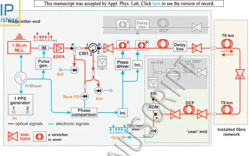
The experimental set-up can be seen in figure 1. Ini-tially we measured the transfer stability using the setup depicted in the grayed out areas18_{. We then implemented}

some minor changes to improve reliability and minimize reflections and we measured the transfer accuracy with this latter setup. An ITU-channel-filtered mode-locked laser (M-Comb, Menlo Systems) with a repetition rate of 100 MHz is used for the time transfer experiments. The repetition rate of the MLL is locked to a signal derived from a hydrogen maser, but the carrier-envelope offset frequency is not stabilized. The ITU channel used in this experiment is channel 44, centred around 1542.14 nm. Filtering to a single ITU channel (100 GHz) reduces the number of optical modes to several hundred correspond-ing to a pulse width of a few ps for Fourier-limited pulses. A total of eleven channel 44 filters were employed; one after the unidirectional EDFA, and one on either side of each bidirectional EDFA in order to reduce spontaneous emission noise and avoid lasing effects.

Three dispersion compensation modules are employed to compensate for a total of approximately 198 km of single-mode fibre (SMF-28). Fibre spools are added to the installed fiber link (159.2 km) to achieve this over-all length. The residual pulse broadening is estimated to be only around two ps. The overall one-way loss of the fiber link including all components is approximately 80 dB whilst the combined gain of the five bidirectional EDFAs (bi-EDFA) is approximately 100 dB. The input power of the first bi-EDFA was set to -25dBm to max-imize the ratio between reflections and useful returned signals on port 3. A signal of around -5 dBm was inci-dent on the photodiode at the user end.

1.56mm LL M

Piezo driver Transmitter end

optical signals electronic signals

‘user’ end

EDFA 3

IM

1 PPS generator

H-Maser

t

t

TIC trigger level Int.

In

1 2

Ret

Out

Pulse gen.

CIR1 1

2

79 km

P2 Delay

line

Int. 40 km SMF

AOM FM

Installed fibre network

Ref

Beat PD

Piezo driver

Phase comparison

P1

79 km DCF

AOM FM

bidir. EDFA

P3

P4

Delay line

DCF

s

s

o

s: stretcher o: oven

FIG. 1. Schematic of the experimental set-up. The phase fluctuations of the fiber link are measured by comparing the optical modes of the local laser with those of the returned laser and suppressed using two fiber stretchers and a temperature-controlled fiber spool. The time transfer performance is characterised by measuring the time intervals using the time marker pulses and an SR620 time interval counter. PD: photodiode; IM: intensity modulator; Pulse gen.: pulse generator; Int.: integrator; EDFA: erbium-doped fiber amplifier; CIR: circulator; det.: photodetector; MLL: mode-locked laser; DCF: dispersion compensating fiber; FM: Faraday mirror; bidir.: bidirectional; PPS: pulse per second; TIC: time interval counter; AOM: acousto optical modulator. Pulse amplification following the photodiodes not shown in this diagram.

on the detection of the optical phase difference between two combs17,19,20_{. The optical beat from which the error}

signal is derived is generated from the optical modes of the local comb and the returned comb, which has been frequency-shifted by 154 MHz due to double-passing an AOM at the user end. In order to achieve temporal over-lap between the two pulse trains at the Beat PD, short fiber patch cords and an optical delay line are used. The fiber link is stabilized employing a fast and a slow feed-back loop. The fast feedback loop (bandwidth of ap-proximately 200 Hz) controls two fibre stretchers (Opti-Phase) with a delay range of 100 ps. The slow feedback loop (time constant of 104_{s) employs a}

temperature-controlled, 12.5 km long fibre spool with a delay range of approximately 13 ns. Whilst the carrier-envelope off-set frequency of the mode-locked laser is not stabilized, as no detection stage is present in the system used for this experiment, fluctuations at time scales much larger than the propagation round trip time are greatly sup-pressed as they are common-mode between the reference and returned pulse trains.

In order to superimpose timing information onto the optical pulse train, an amplitude modulation scheme is

repetition rate detected by the local and remote photo-diodes. However, as only one out of every several tens of thousands pulses is modulated (80,000 in our experi-ment), their magnitude is extremely small. Should this level be still too high for ultra-low noise applications, it would be possible to reduce the modulation index (until proper detection of the marker pulse is no longer pos-sible), further increase the interval between the marker pulses and/or phase lock a good quality local oscillator to the transferred signal with a bandwidth smaller than the inverse of the interval between time marker pulses.

The procedure used to calibrate the time transfer set-up is based on the same concept as in the work described by Krehlik et al.7 _{and a timing model of the set-up is}

shown in figure 2. The absolute time delay between the local time reference (1 PPS generator) and the corre-sponding time marker pulse at the user end is calculated as half of the measured round-trip delay, which can be monitored at the transmitter end, plus a constant cali-bration factor which takes account of any delays which are non-common to the forward and backward directions of the fiber link. The reference output and the return output of the set-up are used to measure the round-trip delay. The calibration factor has to be determined be-fore the time transfer experiment is carried out. The non-common delays t2, t3, t5, t6 and t7 experienced by

the time marker pulses (due to fibre and electrical com-ponents) are defined by the points P1, P2, P3, and P4

shown in figure 1 and figure 2. Since the pulse gener-ator superimposes timing information onto the optical pulse train rather than the PPS generator (PPS-2 Spec-traDynamics), there is a time interval τIn→Ref between

the release of the 1 PPS signal and the arrival of the corresponding optical time marker pulse at the reference output which has to be determined. This time interval can be measured at the transmitter end by comparing the delay between the PPS signal and the time marker pulse at the reference output, and it will be constant dur-ing operation of the time transfer link as the MLL, the pulse generator and the PPS generator are all locked to the hydrogen maser. The time interval τIn_→Ref can be

expressed as the sum of the following time delays expe-rienced by the time marker pulse: tx, which is the sum

of the time it takes the marker pulse to travel from the unknown point where it is when the PPS signal is re-leased to P1, and t2. We denote by τIn_→Out the time

interval between the output pulse at the PPS generator and the electrical pulse detected by the photodetector at the user end (Out), byτRef→Out the time interval

be-tween the pulses detected by the reference (Ref) and user (Out) photodetectors and byτRef_→Ret the time interval

between the pulse detected by the reference (Ref) and the return photodetectors (Ret) after the pulse train has travelled a round trip through the 79.6 km-long optical link. In all cases the detected pulses are amplified to a suitable amplitude (typically 1.5 V) for counting using RF amplifiers and the amplitude was matched, using a

In Ref Ret Out t 3 t₂ τ Fib_F τ Fib_B t 5 t₆ t₇

t_x P

1

P2 P3

P

4

τ

Ref®Out

τ

In®Out

τ

Ref®Ret

fibre link

Transmitter end User end

τ

In®Ref

from PPS generator

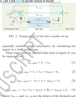
FIG. 2. Timing model of the time transfer set-up.

manually variable optical attenuator, by visualizing the signal on a fast oscilloscope.

These time intervals (dashed blue lines in figure 2) can be expressed as:

τIn→Ref=tx+t2, (1)

τIn_→Out=tx+t3+τFib F+t5, (2)

τRef→Out =−t2+t3+τFib F+t5, (3)

τRef→Ret=−t2+t3+τFib F+ 2t6+τFib B+t7, (4)

whereτFib FandτFib B are the delays of the forward and

the backward directions of the fiber link. Here, there is no difference betweenτFib FandτFib Bdue to the Sagnac

effect, since the transmitter end and user end of the set-up are located in the same laboratory. A small difference betweenτFib F andτFib B may arise due to polarisation

mode dispersion (see table I). Using equations 1–4, the delay between the local time reference signal (PPS gen-erator) and the user timing signal (time marker pulse) can be expressed as:

τIn_→Out=τIn_→Ref+

1

2τRef→Ret+ 1

2(τFib F−τFib B)+ 1 2τc,

(5) whereτc is a calibration factor that takes account of the

non-common paths between the forward and the back-ward directions of the path of the time marker pulses:

τc =−t2+t3+ 2t5−2t6−t7. (6)

In order to determine the calibration factorτc, the local

and the remote modules must be located in the same laboratory. The fiber link is replaced by a variable fiber attenuator which is tuned to give the same attenuation as the fiber link. As a consequence, the difference between

τFib FandτFib Bis negligible and (inserting equations 1, 2

and 4 into equation 5) the calibration factor is given by:

τc = 2τRef′ →Out−τRef′ →Ret, (7)

where the primes indicate that this is the calibration measurement. Hence,τc can be determined by

Sensitivity Uncertainty Source Uncertainty (ps) coefficient contribution (ps)

τIn→Ref 50 1 50

τRef_→Ret 50 0.5 25

PMD 0.6 0.5 0.3

τc 112 0.5 56

Total uncertaintyτIn→Out 80 ps

TABLE I. Uncertainty budget for determiningτIn→Outusing an SR620 time interval counter. The sensitivity factors from equation 5 are taken into consideration. The uncertainty of τcis obtained by adding the contributions of the right side of equation 7 in quadrature. PMD: Polarisation mode disper-sion.

FIG. 3. Residual delay fluctuations of the fiber link for the free-running case (blue line) and the locked case (red line).

known, the absolute delayτIn→Outof any delay-stabilized

fiber link can be determined via equation 5 by measur-ing τIn→Ref and τRef→Ret at the transmitter end. Here,

the time delays are measured using an SR620 (Stanford Research Systems) time interval counter which has an uncertainty for relative time interval measurements of ap-proximately 50 ps. The total uncertainty for determining

τIn_→Out (80 ps, see table I) is obtained by adding all

un-certainty contributions of the terms on the right side of equation 5 in quadrature.

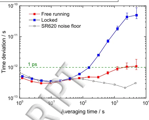
The time transfer stability is determined by measur-ing the time interval between the points Ref and Out of figure 1 using the SR620 time interval counter triggered by the time marker pulses (period 800µs) and averaging over 1000 samples. The trigger level was set to 80% of the marker pulse amplitude. The residual delay fluctu-ations and the corresponding time deviation of the free running (blue traces) and the stabilized fiber link (red traces) can be seen in figure 3 and figure 4 respectively.

The stabilization of the fiber link results in a reduction of the time deviation by a factor of approximately 50 (at 5000 s) compared to the free running link. When the link is stabilized, the time deviation reaches a value of approximately 300 fs at 5 s. The time deviation at this

10 0 10 1 10 2 10 3 10 4 10 -13 10 -12 10 -11 10 -10 Free running Locked

SR620 noise floor

T i m e d e vi a t i o n / s

Averaging time / s

1 ps

FIG. 4. Time deviation of the NPL–Reading fiber link cal-culated from the free-running (blue solid squares) and locked (solid red squares) delay fluctuations shown in figure 3. The measurement limit of the SR620 is also shown (black open squares).

Time interval measurements Signal Time interval (ps)

Ref 163 266 631

Ret 163 564 361

Out 163 395 623

Calculated time delays Delay Time interval (ps) τRef′ →Out 128 992 τRef′ →Ret 297 730

τc= (=39.7±0.1)ns

TABLE II. Results of a time transfer calibration measure-ment. The time delays of interest at the bottom of the table are calculated from the time interval measurements at the top of the table. In order to obtain relative time interval measure-ments, channel A of the time interval counter is triggered by the auxiliary channel 2 output of the PPS generator for all measurements while channel B is sequentially connected to the various signals of interest.

time scale is limited by the residual fluctuations of the SR620 time interval counter.

In order to verify the time transfer accuracy, a total of four calibration measurements (determination ofτc) and

six verification measurements (comparison between pre-diction and direct measurement ofτIn_→Out) were carried

out over the course of several days. The result from one calibration measurement can be seen in table II. The measured time intervals at the top of the table were ob-tained by measuring each time interval for approximately 5 minutes (using the SR620) and subsequently calculat-ing the average value; this is the case in the verification measurements as well. All four calibration measurements were in agreement within their uncertainty of 112 ps; the average value was approximatelyτc=−39.8 ns, the

Signal Time interval (ps)

In 4 152

Ref 163 264 768

Ret 788 384 111

Out 475 804 491

Calculated time delays

Delay Time interval (ps)

τIn→Ref 163 260 616

τRef→Out 1 112 539 723

τRef_→Ret 2 225 119 343

τIn→Out(prediction) (1 275 800.41±0.08)ns

τIn→Out(measurement) (1 275 800.34±0.05)ns

TABLE III. Results of a time transfer verification measure-ment. The predicted value of the delayτIn→Outand the direct measurement ofτIn_→Outagree within their associated uncer-tainties.

was 131 ps.

For the verification measurements the optical path length of the fiber link was stabilized. The result from one verification measurement can be seen in table III. Since the one-way delay of the fiber link is approximately 1.1 ms and the time marker period was set to 800µs, dif-ferent time marker pulses start and stop the time in-terval measurement on the SR620. This has to be ac-counted for when calculating the time delays of interest in table III. To obtain the correct value for τRef_→Out

(τRef_→Ret), 800µs (1.6 ms) have to be added to the

dif-ference between Out and Ref (Ret and Ref). The largest possible time marker repetition rate, that still enables any pulse ambiguity to be resolved in a simple way, was chosen for averaging purposes.

In five of the six verification measurements the direct measurement and the predicted value ofτIn_→Out were in

agreement within their associated uncertainties. Only in one measurement was the difference (−144 ps) slightly larger than the combined one sigma uncertainties. The average deviation between the prediction and the direct measurement was −32 ps, the standard deviation was 104 ps.

In summary, a time transfer technique based on the propagation of an optical pulse train from a mode-locked laser was demonstrated over a 159 km-long installed fiber link. A time transfer stability of approximately 300 fs at 5 s was measured. This performance, which is limited by the residual fluctuations of the SR620 time interval counter, is at a similar level as the state-of-the-art per-formance reported by Krehlik et al.7,21 _using

amplitude-modulated CW lasers. The time transfer accuracy has been measured to be at the 100 ps level. This per-formance was also limited by the SR620 time interval counter. In the future, the accuracy could be improved, potentially to 10 ps, by using a digital storage oscillo-scope rather than a standard time interval counter. This experiment, in conjunction with our previous work17, demonstrates that frequency comb-based fiber transfer

quencies and optical frequencies simultaneously over long telecommunication fiber links with high stability and ac-curacy levels.

Funding. This work is supported by the UK National Measurement System and the European Metrology Re-search Programme (EMRP). The EMRP is jointly funded by the EMRP participating countries within EURAMET and the European Union. The fibre link used in this work is funded by the UK Space Agency. ML acknowledges support from the Engineering and Physical Sciences Re-search Council (EPSRC) through the Centre for Doctoral Training in Applied Photonics. Maurice Lessing is now at Menlo Systems GmbH, Am Klopferspitz 19a, 82152, Martinsried, Germany

1_{B. Bloom, T. Nicholson, J. Williams, S. Campbell, M. Bishof,}

X. Zhang, W. Zhang, S. Bromley, and J. Ye, Nature 506, 71 (2014).

2_{T. Nicholson, S. Campbell, R. Hutson, G. Marti, B. Bloom,}

R. McNally, W. Zhang, M. Barrett, M. Safronova, and G. Strouse, Nature Communications6, 6896 (2015).

3_{I. Ushijima, M. Takamoto, M. Das, T. Ohkubo, and H. Katori,}

Nature Photonics9, 185 (2015).

4_{K. Predehl, G. Grosche, S. Raupach, S. Droste, O. Terra, J.}

Al-nis, T. Legero, T. W. H¨ansch, T. Udem, R. Holzwarth, and H. Schnatz, Science336, 441 (2012).

5_{S. Droste, F. Ozimek, T. Udem, K. Predehl, T. W. H¨ansch,}

H. Schnatz, G. Grosche, and R. Holzwarth, Physical Review Let-ters111, 110801 (2013).

6_{D. Calonico, E. Bertacco, C. Calosso, C. Clivati, G. Costanzo,}

M. Frittelli, A. Godone, A. Mura, N. Poli, D. Sutyrin, G. Tino, M. E. Zucco, and F. Levi, Applied Physics B117, 979 (2014).

7_{P. Krehlik, L. ´Sliwczy´nski, L. Buczek, and M. Lipi´nski, IEEE}

Transactions on Instrumentation and Measurement 61, 2844 (2012).

8 _{L. Sliwczy´}´ _{nski, P. Krehlik, A. Czubla, L. Buczek, and} M. Lipi´nski, Metrologia50, 133 (2013).

9_{D. Piester, A. Bauch, L. Breakiron, D. Matsakis, B. Blanzano,}

and O. Koudelka, Metrologia45, 185 (2008).

10_{O. Lopez, A. Kanj, P.-E. Pottie, D. Rovera, J. Achkar,}

C. Chardonnet, A. Amy-Klein, and G. Santarelli, Applied Physics B110, 3 (2013).

11_{F. Yin, Z. Wu, Y. Dai, T. Ren, K. Xu, J. Lin, and G. Tang,}

Optics Letters39, 3054 (2014).

12_{M. Rost, D. Piester, W. Yang, T. Feldmann, T. W¨ubbena, and}

A. Bauch, Metrologia49, 772 (2012).

13_{B. Wang, C. Gao, W. Chen, J. Miao, X. Zhu, Y. Bai, J. Zhang,}

Y. Feng, T. Li, and L. Wang, Scientific Reports2(2012).

14_{S. M. Raupach and G. Grosche, IEEE Transactions on}

Ultrason-ics, FerroelectrUltrason-ics, and Frequency Control61, 920 (2014).

15_{F. R. Giorgetta, W. C. Swann, L. C. Sinclair, E. Baumann,}

I. Coddington, and N. R. Newbury, Nature Photonics 7, 434 (2013).

16_{L. C. Sinclair, W. C. Swann, H. Bergeron, E. Baumann,}

M. Cermak, I. Coddington, J. D. Deschnes, F. R. Giorgetta, J. C. Juarez, I. Khader, K. G. Petrillo, K. T. Souza, M. L. Den-nis, and N. R. Newbury, Applied Physics Letters109, 15, (2015).

17_{G. Marra, H. S. Margolis, and D. J. Richardson, Optics Express} 20, 1775 (2012).

18_{M. Lessing, H. S. Margolis, C. T. A. Brown, and G. Marra,}

Con-ference on Lasers and Electro-Optics (CLEO),20, 1775 (2015).

19_{Y.-F. Chen, J. Jiang, and D. J. Jones, Opt. Express14, 12134}

(2006).

20_{S. M. Foreman, K. W. Holman, D. D. Hudson, D. J. Jones, and}

J. Ye, Review of Scientific Instruments78, 021101 (2007).

21_{P. Krehlik, L. ´Sliwczy´nski, L. Buczek, J. Ko lodziej, and}

1.5

6

m

m

LL

M

Piezo

driver

optical signals electronic signals

‘user’ end

EDFA

3

IM

1 PPS

generator

H-Maser

t

t

TIC trigger

level

Int.

In

1

2

Ret

Out

Pulse

gen.

CIR1

1

2

79 km

P

Delay

line

Int.

40 km SMF

AOM

FM

Installed fibre

network

Ref

Beat PD

Piezo

driver

Phase

comparison

P

79 km

DCF

AOM

FM

bidir.

EDFA

P

P

Delay

line

DCF

s

o

s: stretcher

In

Ref

Ret

Out

t

3

t

2

τ

Fib_F

τ

Fib_B

t

5

t

6

t

7

t

x

P

P

P

P

τ

Ref

®

Out

τ

Ref

®

Ret

fibre link

Transmitter end

User end

τ

In

®

Re

f

10

0

10

1

10

2

10

3

10

4

10

-13

10

-12

10

-11

Free running

Locked

SR620 noise floor

T

i

m

e

d

e

vi

a

t

i

o

n

/

s

Averaging time / s