Power-port modelling of an in-plane 3 DOF parallel micro-manipulator with feed-forward position control

(1)

University of Twente

EEMCS / Electrical Engineering

Control Engineering

Power-port modelling of an in-plane 3

DOF parallel micro-manipulator with

feed-forward position control

Tijs Lammertink

M.Sc. Thesis

Supervisors

prof.ir. H.J.M.R. Soemers prof.dr.ir. S. Stramigioli ir. B.R. de Jong dr.ir. G.J.M. Krijnen

(2)

(3)

Summary

As part of the Multi Axis MicroStage project (MAMS), a 20-sim model of a 3 DOF parallel micro-manipulator was created. The model serves as a design tool and as verification in order to understand the behaviour of the actual system. The micro-manipulator was fabricated with MEMS technology. One of the possible applications for the manipulator is manipulation of samples in a Transmission Electron Microscope (TEM).

A multibody model of the manipulator was created with 20-sim’s 3D Mechanics Editor. The multibody model contains the rigid bodies (with their positions, masses and inertias), and the kinematic construction of joints and rigid bodies. An equation submodel of the multibody model is exported to 20-sim. The compliant behaviour of the manipulator is added in 20-sim. Stiffness, masses and inertias were estimated on the basis of the physical dimensions of the actual device. The damping has been estimated roughly from measurements and is very low, which is typical for MEMS devices.

The manipulator is actuated by drives. Since it is not trivial what voltage to apply to which comb-drive for movement of the manipulator’s end-effector in a specific direction, a feed-forward position control was designed, which controls the manipulator in the desired coordinates.

Measurements on the real manipulator were performed: The platform deflection was measured for different comb-drive voltages as well as the resonance frequencies. The model was validated with mea-surements, which shows very similar relations between simulated and measured platform deflection as a function of the comb-drive voltages. The difference between simulations and measurements are: 2.3 % in

(4)

(5)

Chapter 1

Introduction

1.1

MAMS Project

This master assignment is part of the Multi-Axis MicroStage project (MAMS). The goal of the MAMS project is design and fabrication of a micro-manipulator with six degrees of freedom (DOF). The most important specifications the manipulator needs to achieve are:

• An enormously high positioning resolution; in the order of 1 nanometre

• Extremely small dimensions; in the order of 1 millimetre

• A very low drift; in the order of 0.1 nanometre per minute

Micro Electro Mechanical Systems (MEMS) process technology is used to fabricate the manipulator. It is a way to create mechanical structures on a silicon chip. MEMS technology is photo lithography based, which is also used in the electrical chip technology.

One of the applications for the micro-manipulator is manipulation of samples in a Transmission Electron Microscope (TEM). The small size of a MEMS device can be beneficial with respect to the conventional manipulator. It enables a larger tilt angle in the gap separating the magnetic lens poles; increasing achievable magnification combined with a large tilt angle. A small device obtains thermal equilibrium much faster. Thermal drift, in occurrence of temperature changes, stabilises quicker. Furthermore, the eigenfrequencies of a small device are very high. Firmly connected to the TEM column, the manipulator will nicely follow the movements of the electron beam due to vibrations of the TEM.

As part of the study on a 6 DOF manipulator, a parallel in-plane manipulator with 3 DOF is fabricated. It enables in-plane translation (alongxandy) and in-plane rotation (aboutz). Together with an out-of-plane manipulator, which enables out-of-out-of-plane movements (translation alongzand rotation aboutxandy), 6 DOF movements are possible.

1.2

Goal of the assignment

The goal of this assignment was to create a dynamic model of an in-plane 3 DOF parallel manipulator in 20-sim. The manipulator consists of three actuators, connected in parallel to an end-effector through flexures. Actuation is based on electrostatic attraction in a so-called comb-drive in pull-pull configuration. The end-effector is a platform that is controlled in the translational (alongxandy) and rotational coordinates (aboutz). The model serves as a design tool and as verification in order to understand the actual system’s behaviour. Special attention is paid to power-port modelling of the three flexures that suspend the end-effector in the manipulator.

(8)

Since it is not trivial what voltage to apply to which comb-drive for movement of the platform in a specific direction, a feed-forward position control is to be designed, which computes the comb-drive deflection and actuation voltage as a function of the desired platform coordinates.

1.3

Report outline

(9)

Chapter 2

Manipulation concepts

In this chapter, two manipulation concepts of a 6 DOF manipulator are explained (see also [5]). In Para-graph 2.1, a conceptual analysis of both manipulators is made. The identification of rigid bodies and flexures is treated in Paragraph 2.2.

2.1

Two manipulation concepts

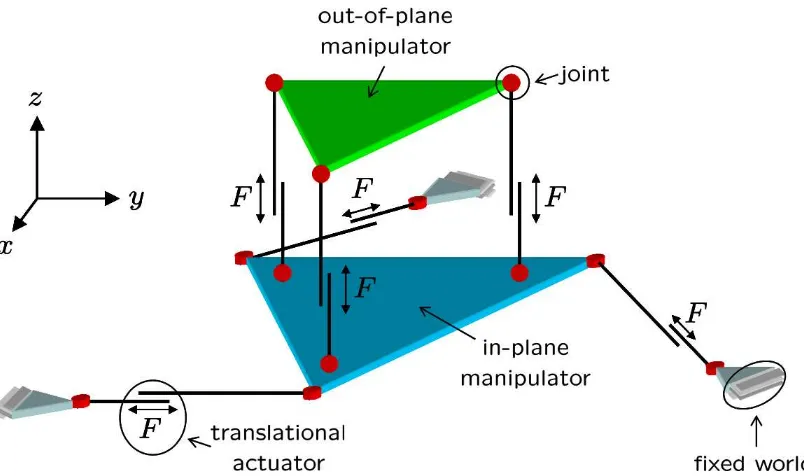
Figure 2.1 shows two manipulation concepts: the in-plane 3 DOF parallel manipulator can be ‘stacked’ on top of the out-of-plane 3 DOF parallel manipulator, or it can be done the other way around. The in-plane manipulator enables translation alongxandyand rotation aboutz. The out-of-plane manipulator enables rotation aboutxandyand translation alongz. This series connection of both 3 DOF manipulators results in a 6 DOF manipulator.

The concept from figure 2.1(a) enables in-plane movement of the bottom platform and out-of-plane movement of the top platform. The bottom platform is connected to three ‘arms’ at its corners. Each arm is connected to the fixed world. The translational actuators exert forces on the platform through joints. In the figure, the joints are represented by circles, but in reality flexures transfer forces to the platform. The top platform is also connected to three arms on its corners. The arms are fixed to the bottom platform through joints. Translational actuators exert forces on the platform through joints.

The concept of figure 2.1(b) enables out-of-plane movement for the outer platform and in-plane move-ment of the inner platform.

2.2

Analysis of the in-plane manipulator

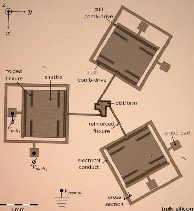
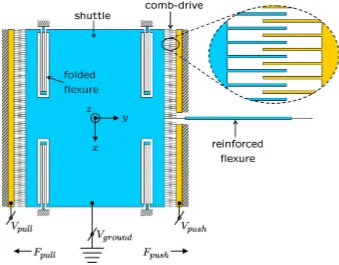
Figure 2.2 shows a photo of the in-plane manipulator through an optical microscope. The outer dimensions are4.5×5.2 mmand the design has a 120° point-symmetry. In the centre, the end-effector (platform) is located. Reinforced flexures connect the platform to so-called shuttles. Each shuttle is suspended by four folded flexures and actuated by two comb-drives in pull-pull configuration.

(10)

(a) Out-of-plane manipulator ‘stacked’ on in-plane manipulator. Out-of-plane manipulator is constrained for in-plane movements (= translation alongxandyand rotation aboutz) and in-plane manipulator is constrained for out-of-plane movements (= translation alongzand rotation aboutxandy)

(b) In-plane manipulator ‘stacked’ on in-plane manipulator. Out-of-plane manipulator is constrained for in-plane movements (= translation alongxandyand rotation aboutz) and in-plane manipulator is constrained for out-of-plane movements (= translation alongzand rotation aboutxandy)

(11)

ANALYSIS OF THE IN-PLANE MANIPULATOR 5

(12)

Figure 2.3: Schematic figure of an arm and a close-up of a comb-drive

Comb-drive

Figure 2.3 shows an on-scale schematic figure (scale 52:1) of one ‘arm’ and a close-up of a comb-drive (scale 420:1). The arm consists of a shuttle, two comb-drives, four folded flexures and a reinforced flexure. A comb-drive is a linear motor that consists of a movable and a stationary set of comb-fingers. When a voltage is applied to the comb-drive, an electrostatic force is generated, and as a result the comb fingers attract each other in they-direction. The electrostatic forces between the fingers inx-direction compensate each other. The comb-drive deflection depends on the stiffness of the folded flexures and the reinforced flexures. The relation between force and voltage is quadratic:

Fcomb=

nǫh g V

2

comb (2.1)

Withnthe number of fingers,ǫthe dielectric constant of the medium between the fingers, which is air or vacuum,hthe height of the comb-fingers andgthe gap between the fingers.

A comb-drive can only generate a force in one direction, since it can only attract its fingers (two opposite charges always attract each other). Therefore, the comb-drives on each shuttle are configured in pull-pull configuration to enable movement in positive as well as negative direction. One comb-drive pulls at one side of a shuttle and the other comb-drive pulls at the other side. However, the comb-drives that ‘push’ the platform are called push drives, and the drives that ‘pull’ the platform are called pull comb-drives, to distinguish between them. The force due to both comb-drives is calculated as follows:

        

       

Fpush=

nǫh g V

2

push

Fpull=

nǫh g V

2

pull

Fpull=−Fpush

⇒ Fpush=

nǫh g

¡

Vpush2 −Vpull2

¢

(13)

ANALYSIS OF THE IN-PLANE MANIPULATOR 7

(a)kg= 12EI

l3

f

(b)kg= 24EI

l3

f

(c)kg= 12EI

l3

f

Figure 2.4: Folded flexure

Folded flexures (comb-drive and shuttle suspension)

A folded flexure is an element with four combined flexures of lengthlf to make it suitable for parallel guiding and constrain rotational movements. Moreover, the shortening effect in longitudinal direction has been compensated. Figure 2.4(a) shows one flexure; it has a guiding stiffness (kg) of12EI_l3

f

, withIthe area

moment of inertia of the folded flexure, andEYoung’s modulus of silicon. Figure 2.4(b) shows two parallel flexures; together they have a guiding stiffness that is two times bigger than one flexure: 24EI

l3 f

. A folded

flexure (Figure 2.4(c)) is in fact a series construction of two times two parallel flexures. The outer two flexures, as well as the inner two flexures, are parallel to each other. The two inner flexures and two outer flexures are in series to each other. Hence the guiding stiffness of one folded flexure becomes two times smaller than that of two parallel flexures, so it has the same guiding stiffness as one flexure has: 12EI

l3 f

.

Each shuttle is suspended with four folded flexures in parallel, which have a combined guiding stiffness that is simply four times bigger:48EI_l3

f .

The same story holds for the longitudinal stiffness (kl). A folded flexure has the same longitudinal stiffness as one flexure: EA_l

f . The combined longitudinal stiffness of four folded flexures is again four times bigger:4EA

lf .

Trench

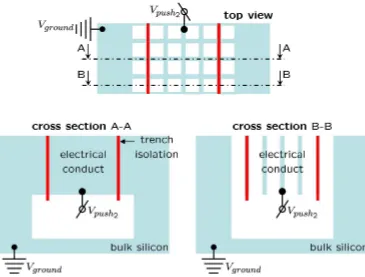
Figure 2.5 shows a schematic top view and two schematic cross sections of a trench (the location is shown in Figure 2.2). Trenches separate different potentials and define regions serving as electrical connections to the comb-drives. The so-called twin-etching method requires that the shuttles and the platform contain square holes. The cross section shows that the trench isolation electrically isolates the trench from the ground potentialVground. Mechanically, the trench is fixed to the bulk. The probe pad potentialVpush2is

transferred to the stationary fingers of the comb-drive through the trench. The ground potential is transferred to the movable fingers of the comb-drive via the bulk, and through the folded flexures.

Assumptions

(14)

Figure 2.5: Schematic cross sections of a trench isolated region

and 5 DOF constrained. The longitudinal stiffness is in the order of104_{bigger than the guiding stiffness,}

so the folded flexures are assumed to be rigid in the longitudinal direction. TheRzrotational stiffness (see Figure 2.3) that the shuttle feels due to the four folded flexures is very big, because of the relatively large distance between two neighbouring folded flexures. TheRxandRytilt stiffness that the shuttle feels is also very big, because of the use of four folded flexures instead of one or two.

Usually, flexures allow torsional movements due to torsion stiffness. This is undesirable when only in-plane movements are actuated, as in this manipulator. But since the parallel construction of three flexures (that connect the platform to the shuttles) does not allow out-of-plane movements, torsion movements of the flexures are constrained. Hence, only the in-plane movements of the flexure are assumed to be compliant and a 3 DOF model of the flexure will be sufficient.

(15)

Chapter 3

Flexure model

In this chapter, the flexure model is addressed. Paragraph 3.1 shows that it is important to choose symmetric coordinates for the stiffness matrix of a 3 DOF flexure. In Paragraph 3.2 a 3 DOF flexure is constructed from 1D springs in 20-sim, and it will be shown that it is impossible to construct a symmetric leaf spring from 1D springs. In Paragraph 3.3 a solution is given to describe the stiffness matrix in symmetric coordinates, but still using an asymmetric joint-structure to construct the flexure. In Paragraph 3.4 the solution is validated by simulations. The manipulator has reinforced flexures which are treated in Paragraph 3.5.

3.1

Choosing symmetric stiffness matrix coordinates

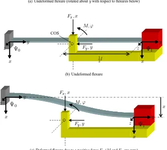
Figures 3.1(a) and 3.1(b) show an undeformed flexure, which is clamped to the fixed world at the left side. At the right side, a rigid body is connected. A massless construction is connected to the bottom of the rigid body. The in-plane forces are applied on the centre of the spring. Usually a flexure is only constrained (to a certain extent) for translation alongzand rotation aboutx. However, since the parallel construction of three flexures in the manipulator does not allow torsional movements, choice is made not to consider torsional stiffness abouty. Hence, the flexure is assumed to be constrained in the out-of-plane directions (3 DOF) and unconstrained in the in-plane directions (3 DOF).

The flexure in Figures 3.1(a) is rotated aroundy with respect to the flexure in Figures 3.1(b). The stiffness matrix of the flexure, around equilibrium and for small deformations, reflected to a point aty= 1₂l

(in its centre of stiffness (COS)) is derived in Appendix B.2:

Kc =

      EI

l 0 0

0 12EI

l3 0

0 0 EA

l       (3.1)

The force-deflection relation for this flexure (for small deflections) is:

   M Fx Fy   =Kc

   ϕ xc yc    (3.2)

The energy function of this flexure (for small deflections) is quadratic:

E= 1 2

h

ϕ xc yc

i Kc    ϕ xc yc   = 12

EI l ϕ

2

c + 6

EI l x

2

c+12

EA l y

2

(16)

x x

y y

z z

l

Ψ

0

Ψ

1

(a) Undeformed flexure (rotated aboutywith respect to flexures below)

x x

y y

z z

1 2l

Ψ

0

Ψ

1

Fx, x

Fy, y

M, ϕ

COS

(b) Undeformed flexure

x

x y

y

z

Ψ

₀

Ψ

1 Fx, x

Fy, y

M, ϕ

(c) Deformed flexure due to a positive forceFx(MandFyare zero)

x

y

z

ϕ

Ψ

0

Ψ

1

Fx, x

Fy, y

M, ϕ

(d) Deformed due to a positive torqueM(FxandFyare zero) in world orientation

(17)

CHOOSING SYMMETRIC STIFFNESS MATRIX COORDINATES 11

x

y

z

ϕ

Ψ

0

Ψ

1

Fx, x

Fy, y

M, ϕ

(e) Deformed due to a positive torqueM(FxandFyare zero) in body orientation

x

y

z

ϕ

1 2ϕ

Ψ

0

Ψ

1

Fx, x

Fy, y

M, ϕ

(f) Deformed due to a positive torqueM(FxandFyare zero) with symmetric orientation

Figure 3.1: Flexure

Figure 3.1(c) shows the same flexure with a deformation due to a positive force inx-directionFx, (M and

Fyare zero). According to the symmetric stiffness matrix, only a deflection inx-direction results.

Figure 3.1(d) shows the flexure with a deformation due to a positive torqueM, (FxandFyare zero). The only deformation is a rotationϕ. The orientation of the forces and torque is chosen such, that it coincides with world coordinates (Ψ0). A flexure is a symmetric element in reality, because it does not

matter whether the left side of the flexure is clamped and the forces affect the right side, or the other way around; the deflection stays the same in both cases. However, the flexure is not modelled symmetrically with this choice of orientation of forces and torque, because it does matter whether the flexure is viewed from right to left or from left to right. Imagine that the two terminals of the spring are swapped, i.e.:

• Instead of the left side, the right side is clamped to the fixed world

• Instead of the right side, the mass is connected on the left side

• The flexure is turned around 180°

Then the flexure in Figure 3.1(e) results. But now, the coordinates are defined differently. In fact, the orientation of the forces is now chosen such, that it coincides with the coordinates of the rigid body (Ψ1).

In general, the orientation of the forces can be chosen in infinitely many ways, but only one choice leads to a symmetrically modelled flexure, which is exactly in the ‘middle’ of both orientations (Ψc) (see Figure 3.1(f)). The orientation of this symmetric coordinate system coincides with the orientation of world coordinates, but rotated+1

2ϕ. And it also coincides with the orientation of body coordinates, but rotated

(18)

does result in the same spring behaviour. Hence, the flexure is modelled symmetrically. However, the stiffness properties have become dependant on the angular deflectionϕ.

3.2

Construction of a flexure model, based on 1 DOF springs

The body-editor is a graphical editor in which a rigid body model (or multibody model) can be created. In such a model, rigid bodies (with a certain mass, inertia and centre of mass (COM)) can be connected to each other through joints, in a user friendly way. Compared to modelling rigid bodies with 6-dimensional bond graphs, modelling with the body-editor is much easier, faster and less sensitive to mistakes. Currently, only 1-dimensional joints were implemented in the body-editor. In a later stage, the program will be expanded with multidimensional joints, since the body-editor is still in development.

Springs are not yet implemented in the body-editor. The way to model a 1D spring is to use a joint in the body-editor and connect a spring to the power port of the joint in 20-sim. In principle, a 1 DOF joint is an ideal joint, representing infinite stiffness in all other directions. Each 1 DOF joint may have its own power-port (consisting of an effort and flow) in 20-sim, to which for example dampers or springs can be connected. For mechanical translation, the effort is force and the flow is velocity. For mechanical rotation, the effort is torque and the flow is angular velocity. If a stiffness (C-type element) is connected to the power-port of a joint, the joint behaves as an ideal spring. The C-type element integrates the velocity to a deflection (x=Rvdt) and, in the case of a linear stiffness, multiplies the deflection with the stiffness (kx·x=Fx), which is equal to the resulting force. More generally, the force is the partial derivative of the energy function of the spring, no matter whether its stiffness is linear or non-linear:Fx(x) =∂E_∂x.

To model the compliant flexure behaviour, the flexure is seen as two massless rods, with a 3 DOF spring in between. There are two methods to define a multidimensional spring in the body-editor. Method 1 (which is the normal method) is connecting a 6 DOF C-element to the power interaction ports of two rigid bodies and constrain the out-of-plane DOFs. Rigid bodies may have such a 6 DOF power interaction port, which appears in the resulting equation submodel in 20-sim. To this port, a multidimensional force (and/or torque) source may be connected for example.

Method 2 is constructing the spring from a series connection of 1D joints and let the axes of the joints cross in one point. A 3 DOF flexure, which is constrained in the out-of-plane directions, can be constructed from a series connection of three 1 DOF joints. However, in general a 6 DOF spring cannot be constructed in this way, because it is well-known that a series connection of three 1D rotational joints always gives problems (the order does matter and the construction may end up in a gimbal lock, for example). But since method 1 gave some numerical problems in simulations (drift in the spring position as well as numerical instabilities), method 2 is still used. The joints that construct an in-plane flexure would logically be the three in-plane joints: two translational (alongxandy) and one rotational (aboutz). However, other constructions are possible, for example two rotational joints and a translational joint in between (see Appendix B.3).

A series connection of translational 1D joints does not give problems. The order of joints does not matter, as is shown in Figures 3.2(a) and 3.2(b); the distance between the rigid body and the fixed world is the same for both multidimensional joints. A problem arises when rotational joints are involved. For example, when two translational joints and one rotational joint are connected in series. In this case, it does matter in which order the joints are connected, because the distance between the rigid body and the fixed

(a)x,y (b)y,x (c)y,x,ϕ (d)ϕ,y,x

(19)

CONSTRUCTION OF A FLEXURE MODEL, BASED ON 1 DOF SPRINGS 13

world is different. This is shown in Figures 3.2(c) and 3.2(d). Two different orders of joints are shown here (but more different orders can be thought of).

Mathematically the problem comes out as follows. Matrix multiplications are in general not commuta-tive, but in the special case of homogeneous matrices, which only consist of translations, matrix multipli-cations are commutative:

H(x) =



 

1 0 x

0 1 0

0 0 1





 H(y) =



 

1 0 0

0 1 y

0 0 1





 (3.4)

H(x)H(y) =H(y)H(x) =



 

1 0 x

0 1 y

0 0 1





 (3.5)

However, matrix multiplications of homogeneous matrices, consisting of rotations and translations are in general not commutative:

H(y)H(x)H(ϕ)=₆ H(ϕ)H(y)H(x) (3.6) WithH(ϕ)a homogeneous matrix, only consisting of a rotation:

H(ϕ) =



 

cos(ϕ) sin(ϕ) 0

−sin(ϕ) cos(ϕ) 0

0 0 1





 (3.7)

Figure 3.3(a) shows a multibody model from a flexure that is constructed by a series connection of joints in the order(x_→y_→ϕ). Figure 3.3(b) shows a multibody model from a flexure that is constructed by a series connection of joints in the order(ϕ→x→y). The joints are interconnected with dummy bodies, having zero mass and inertia. The flexure is clamped to the fixed world on the left side, and on the right side a rigid body is connected to the flexure.

When the joints are connected in the order(x→y→ϕ), the stiffness matrix seems to be defined in world orientation; the forcesFx, Fy and torqueM (which are related to the deflectionx, yand rotation

ϕby this stiffness matrix) seem to have the same orientation as world coordinates. Hence, this flexure is equivalent to the flexure in Figure 3.1(d) and is called the ‘world-flexure’. When the joints are connected in the order(ϕ_→x_→y), the stiffness matrix seems to be defined in body orientation; the forcesFx, Fy and torqueM (which are related to the deflectionx, yand rotationϕby this stiffness matrix) seem to have the same orientation as body coordinates. Hence, this flexure is equivalent to the flexure in Figure 3.1(e) and is called the ‘body-flexure’. The three joints cannot be connected in such a way that the resulting flexure is symmetrically modelled, like the flexure in Figure 3.1(f).

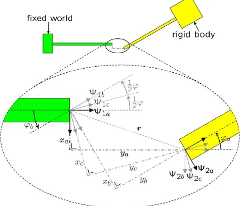
Figure 3.4(a) shows the flexure again, with three different choices of stiffness matrix coordinates. The Ψacoordinates are asymmetric and related to the coordinates from Figure 3.3(a) and 3.1(d). TheΨb coor-dinates are asymmetric and related to the coorcoor-dinates from Figure 3.3(b) and 3.1(e). TheΨccoordinates are the only symmetric coordinates and related to the coordinates from Figure 3.1(f).

Infinitely many choices can be made to measure the distancexandybetween the spring terminals (see Figure 3.4(b)), as long asx2₊_y2 ₌ _r2 _{holds. Viewing the flexure from left to right, a series of four}

coordinate changes is performed: first a rotationH(ϕ1), then a translationH(x), then a translationH(y)

and then a rotationH(ϕ2):H =H(ϕ1)H(x)H(y)H(ϕ2). The first rotationϕ1can be chosen in the range

[0 :ϕ]. The second rotationϕ2is also in the range[0 :ϕ], but should be equal toϕ−ϕ1, to make the total

rotationϕ.

The only symmetric coordinates from this range are theΨccoordinates (see Figure 3.4(c)). Viewing the flexure from left to right, the coordinate changes areHc =H(1₂ϕc)H(xc)H(yc)H(1₂ϕc). Looking from right to left, the coordinate changes areH(1

2ϕc)H(yc)H(xc)H( 1

2ϕc). This is the same, but onlyxandy

are switched. However, this does not matter, as mentioned before (see Figures 3.2(a) and 3.2(b)).

(20)

(a) Series connection in the order(x→y→ϕ) (b) Series connection in the order(ϕ→x→y)

(c) Symbolic representation (d) Symbolic representation

Figure 3.3: Flexure model, constructed from 1 DOF springs

(a) Three different choices of force/torque coordinates

(b) Infinitely many choices of force/torque coordinates (c) Symmetric force/torque coordinates

(21)

SYMMETRIC MODEL OF A FLEXURE 15

3.3

Symmetric model of a flexure

The energy function of the flexure is expressed in symmetricΨc coordinates. However, symmetric co-ordinates are not available, in contrast to asymmetricΨa coordinates (or the asymmetricΨb coordinates, depending on the order of the 1D joints, as explained in the previous paragraph). A solution is to rewrite the energy function (Equation 3.3) and express it inΨacoordinates:

E=1₂EI

l ϕ

2

c+ 6

EI l x

2

c+12

EA l y

2

c (3.8)

The relation between(xc, yc)and(xa, ya)is a rotation of coordinates as can be seen in Figure 3.5:

  

 

ϕc=ϕa

"

xc

yc

#

=R1 2ϕ " xa ya # ⇒     

ϕc =ϕa

xc=xacos(1₂ϕa) +yasin(1₂ϕa)

yc=−xasin(1₂ϕa) +yacos(1₂ϕa)

(3.9)

And substituted in the energy function:

E= 1₂EI

l ϕ

2

a+ 6

EI l

¡

xacos(12ϕa) +yasin(12ϕa)

¢2

+1₂EA

l

¡

−xasin(12ϕa) +yacos(12ϕa)

¢2

(3.10)

To find the force vector, the energy function has to be differentiated to the coordinates:

M = ∂E

∂ϕa = µ EI l ¶ ϕ+ µ

−3EIsin(ϕ)

l3 +

EAsin(ϕ) 4l

¶

x2_a

+

µ

6EIcos(ϕ)

l3 −

EAcos(ϕ) 2l

¶

xaya+

µ

3EIsin(ϕ)

l3 −

EAsin(ϕ) 4l

¶

y2a

(3.11)

Fx=

∂E ∂xa

=

Ã

12 cos2₍1 2ϕ)EI

l3 +

sin2(1₂ϕ)EA l

!

xa+

µ

6 sin(ϕ)EI

l3 −

sin(ϕ)EA

2l

¶

ya (3.12)

Fy=

∂E ∂ya

=

µ_{6 sin(}_ϕ₎_EI

l3 −

sin(ϕ)EA

2l

¶

xa+

Ã

12 sin2₍1 2ϕ)EI

l3 +

cos2₍1 2ϕ)EA

l

!

ya (3.13)

These energy-conservative spring equations are put in the C-type element. Since they are non-linear, they cannot be rewritten to matrix from, like in Equation 3.2.

When the flexure rotation is zero and only a deflection occurs, the coordinate systems overlap and the energy functions are the same:

E= 6EI

l x

2₊1 2

EA l y

2 _(3.14)

(22)

The calculation can be performed for theΨb coordinates as well. But in that case, the stiffness matrix coordinate transformation is a rotation of₋1₂ϕinstead of+1

2ϕ. The energy function then becomes:

E=1₂EI

l ϕ

2

b+ 6

EI l

¡

xbcos(−12ϕb) +ybsin(−12ϕb)

¢2

+1₂EA

l

¡

−xbsin(−12ϕb) +ybcos(−12ϕb)

¢2

(3.15) In the next paragraph a simulation shows that this solution works.

3.4

Simulation of asymmetric and symmetric flexures

To show that the orientation of coordinates of the stiffness matrix matters, a world-flexure (order of springs is(x_→y_→ϕ), see Figure 3.6(a)) is compared with a body-flexure (order of springs is(ϕ_→x_→y), see see Figure 3.6(b)). In the next paragraph both flexures are simulated with a linear spring/stiffness matrix (hence a quadratic energy function). In Paragraph 3.4.2 both flexures are simulated again, but with corrected energy functions (see Equations 3.10 and 3.15). Then, the flexures get similar behaviour and are symmetric.

3.4.1

Asymmetric flexures

The stiffness matrix from Equation 4.19 has been connected to both flexures:

K=



 

1.09_·10−8 ₀ ₀

0 0.0584 0

0 0 34404





 (3.16)

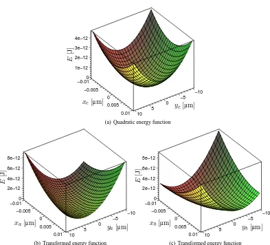
They both have a length of 1 mm. The rigid bodies have the mass and inertia of the platform (2.11 µg, see Paragraph 4.3.4). Some damping is modelled to damp out the oscillations. The energy functions of the flexures are quadratic:

E= 5.45_·10−9_ϕ2

c+ 0.0292x2c+ 17202yc2 (3.17)

Figure 3.7(a) shows a 3D-plot of this energy function as a function ofxcandyc, withϕc = 0.1°. Figure 3.8 shows a 3D-plot of this energy function as a function ofxcandyc, withϕc = 0°. Visually they are the same, but the second one has an ‘offset’ of5.45_·10−9

·¡0.1π

180

¢2

= 1.66_·10−14_{J. The spring equations of}

this leaf spring are:

M′ _{= 1}_.₀₉_·₁₀−8_ϕ

c Fx′ = 0.0584xc Fy′ = 34404yc (3.18)

The accent distinguishes between the force and torque at the springs (with′_{), and the applied force and}

torque at the end (without′_{) (see Figures 3.9(e) and 3.9(f)).}

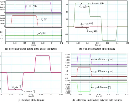
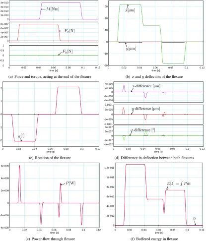
A certain force and torque(M, Fx, Fy)(in body orientation) acts at the end of both flexures (see Fig-ure 3.9(a)). The deflection of the body with respect to its origin (its undeformed position) is given in Figures 3.9(b) and 3.9(c). Between 0.015 and 0.04 seconds only a forceFxis applied. Between 0.045 and

(a) World-flexure: series connection in the order(x→

y→ϕ)(stiffness matrix is defined in world orientation)

(b) Body-flexure: series connection in the order(ϕ→

x→y)(stiffness matrix is defined in body orientation)

(23)

SIMULATION OF ASYMMETRIC AND SYMMETRIC FLEXURES 17

0.065 seconds the same force is applied, together with a torqueM such that the rotationϕis just cancelled and a deflectionx= 13.7µmremains. This can be calculated as follows:

(

Fx= 0.8µN

M = 4·10−10_Nm ⇒

(

F′

x= 0.8µN

M′₌_M ₋_F

x12l= 0

⇒

(

x′₌ Fx′ kx =

0.8µN

0.0584 = 13.7µm

ϕ′ _{= 0} ⇒

(

x=x′₊1

2lsin(ϕ′) = 13.7µm

ϕ=ϕ′ _{= 0}

(3.19)

The applied force at the end of the flexure creates a torque in the middle, which exactly compensates for the applied torque at the end. Between 0.07 and 0.095 seconds only a moment is applied.

Schematic representations with deformed springs of the flexures at different time instances are given in Figures 3.9(e) and 3.9(f). To give insight in which 1D spring is deformed, undeformed 1D springs (springs which do not feel any force at that moment) are not shown in these figures.

The deflections of both flexures indeed differ. The difference between the deflections is shown in Fig-ure 3.9(d), which is 0.036 µm and 0.50 µm inxandy-direction. Between 0.01 and 0.04 seconds, only a force inx-direction is applied, which results in a torque and force at the centre of the flexure. For the world-flexure holds thatFx is acting totally on thex-spring, but for the body-flexure holds thatFx is divided between thex-spring andy-spring. Therefore, thex-deflection of the world-flexure is bigger than that of the body-flexure.

As long as the rotation is zero, the coordinate systems in which the stiffness matrices are described, overlap. This is obvious in Figure 3.4(a). Whenϕ = 0thenxa = xb = xc andya = yb = yc. The simulation also shows this between 0.045 and 0.065 seconds; the flexure deflections are the same.

The difference is only 0.036 µm and 0.50 µm in xandy-direction, but increases rapidly for bigger rotations. For rotations about five times bigger (_±10°), the difference is already 4.8 µm and 13 µm.

3.4.2

Symmetric flexures

The simulation is performed again, but the stiffness matrices are replaced by the non-linear stiffness equa-tions (Equaequa-tions 3.11, 3.12 and 3.13). The energy funcequa-tions of the springs are calculated for this numerical example. The energy function of the world-flexure is (see Equation 3.10):

Eworld= 5.45·10−9ϕ2a+ 2.92·10−2(xacos(1₂ϕa) +yasin(1₂ϕa))2

+ 1.72_·105(₋xasin(₂1ϕa) +yacos(1₂ϕa))2 (3.20) Figure 3.7(b) shows a 3D-plot of this energy function as a function ofxa andya forϕa = 0.1° (and in Figure 3.8 withϕa = 0°). The energy function is quadratic forxa andyawhenϕ= 0, but deviates more and more from the quadratic energy function whenϕincreases. The energy function of the body-flexure is (see Equation 3.15):

Ebody = 5.45·10−9ϕ2b+ 2.92·10−2(xbcos(1₂ϕb)−ybsin(1₂ϕb))2

+ 1.72·105(xbsin(12ϕb) +ybcos(12ϕb))

2 _(3.21)

Figure 3.7(c) shows a 3D-plot of this energy function as a function ofxb andyb forϕb = 0.1° (and in Figure 3.8 withϕb= 0°).

Figures 3.10(b) and 3.10(c) show that statically the deflections are the same. The small differences between the deflections that are shown in Figure 3.10(d) only occur during changes in force and torque. Because of the small rotations possible in the manipulator, only a small error is made when asymmetric flexures are implemented instead of the symmetric ones.

(24)

–10 –5 0 5 10 –0.01 –0.005 0 0.005 0.01 0 1e–12 2e–12 3e–12 4e–12

yc[µm]

xc[µm]

E

[J

]

(a) Quadratic energy function

–10 –5 0 5 10 –0.01 –0.005 0 0.005 0.01 0 2e–12 4e–12 6e–12 8e–12

ya[µm]

xa[µm]

E

[J

]

(b) Transformed energy function

–10 –5 0 5 10 –0.01 –0.005 0 0.005 0.01 0 2e–12 4e–12 6e–12 8e–12

yb[µm]

xb[µm]

E

[J

]

(c) Transformed energy function

Figure 3.7: Energy function as a function ofxandy, withϕ= 0.1°

–10 –5 0 5 10 –0.01 –0.005 0 0.005 0.01 0 1e–12 2e–12 3e–12 4e–12 y[µm] x[µm] E [J ]

(25)

SIMULATION OF ASYMMETRIC AND SYMMETRIC FLEXURES 19

0 1e-010 2e-010 3e-010 4e-010

0 2e-007 4e-007 6e-007 8e-007

0 0.02 0.04 0.06 0.08 0.1 0.12

time {s} -1

-0.5 0 0.5 1

M[Nm]

Fx[N]

Fy[N]

(a) Force and torque, acting at the end of the flexure

0 0.02 0.04 0.06 0.08 0.1 0.12

time {s} -20

-10 0 10 20

30 xworld[µm]

xbody[µm]

yworld[µm]

ybody[µm]

(b)xandydeflection of the flexure

0 0.02 0.04 0.06 0.08 0.1 0.12

time {s} -2

-1 0 1 2

ϕbody[°]

ϕworld[°]

(c) Rotation of the flexure

-0.005 0.005 0.015 0.025 0.035

-0.1 0.1 0.3 0.5

0 0.02 0.04 0.06 0.08 0.1 0.12

time {s} -0.0025

-0.002 -0.0015 -0.001 -0.0005 0 0.0005

x-difference[µm]

y-difference[µm]

ϕ-difference[°]

(d) Difference in deflection between both flexures

(e) World-flexure(x→y→ϕ), at different time instances

(f) Body-flexure(ϕ→x→y), at different time instances

(26)

0 1e-010 2e-010 3e-010 4e-010 0 2e-007 4e-007 6e-007 8e-007

0 0.02 0.04 0.06 0.08 0.1 0.12

time {s} -1 -0.5 0 0.5 1 M[Nm] Fx[N] Fy[N]

(a) Force and torque, acting at the end of the flexure

0 0.02 0.04 0.06 0.08 0.1 0.12

time {s} -20 -10 0 10 20 30

x[µm]

y[µm]

(b)xandydeflection of the flexure

0 0.02 0.04 0.06 0.08 0.1 0.12

time {s} -2 -1 0 1 2 ϕ[°]

(c) Rotation of the flexure

-4e-006 -2e-006 0 2e-006 4e-006 -0.0001 -5e-005 0 5e-005 0.0001

0 0.02 0.04 0.06 0.08 0.1 0.12

time {s} -4e-007 -2e-007 0 2e-007 4e-007

x-difference[µm]

y-difference[µm]

ϕ-difference[°]

(d) Difference in deflection between both flexures

0 0.02 0.04 0.06 0.08 0.1 0.12

time {s} -4e-009 -2e-009 0 2e-009 4e-009 6e-009 P[W]

(e) Power-flow through flexure

0 0.02 0.04 0.06 0.08 0.1 0.12

time {s} 0 2e-012 4e-012 6e-012 8e-012 1e-011 1.2e-011

E[J] =RP dt

0

(f) Buffered energy in flexure

(27)

REINFORCED FLEXURES 21

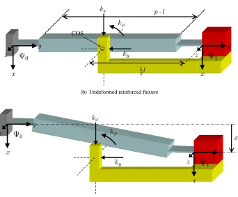
3.5

Reinforced flexures

Instead of flexures with a fixed thickness, reinforced flexures transfer forces to the platform. These flexures have a reinforced mid-section which not only leads to an increase in all stiffnesses (see Soemers [7]):

K=



 

kϕ 0 0

0 kx 0

0 0 ky



 =



      

EI l

µ ₁

1₋p

¶

0 0

0 12EI

l3

µ ₁

1−p3

¶

0

0 0 EA

l

µ

1 1−p

¶ 

      

(3.22)

But also leads to a slower decrease inkyas a function of thex-displacement, according to v.Eijk [4]:

ky

ky,0

= 1

1 + 12x

2

(1₋p)Bd2

(3.23)

With:

B= 700 (1 +q)(1 + 3q+ 3q

2₎3

1 + 10q+ 45q2_{+ 105}_q3_{+ 105}_q4 and q=

p

1−p (3.24)

(28)

x x

y y

z z

l

Ψ

0

Ψ

1

p·l

(a) Undeformed reinforced flexure (rotated aboutywith respect to flexures below)

x x

y y

z z

1 2l

Ψ

0

Ψ

1

p_·l kx

ky

kϕ

COS

(b) Undeformed reinforced flexure

x

x y

y

z

Ψ

₀

Ψ

1 kx

ky

kϕ

(c) Deformed reinforced flexure due to a positive forceFx(MandFyare zero)

(29)

Chapter 4

Power-port modelling & simulation

In this chapter the 20-sim model of the manipulator is addressed. Paragraph 4.1 explains the multibody model that was created in the body-editor. In Paragraph 4.2 the 20-sim model is treated. Parameters like masses, inertias and stiffnesses are calculated in Paragraph 4.3. In Paragraph 4.4 the stiffness and resonance frequencies of the manipulator are simulated with 20-sim.

4.1

Multibody model

The multibody model of the in-plane manipulator is given in Figure 4.1. The dimensions of the squares in the grid are0.5_×0.5mm. Three arms are connected to a triangular platform in parallel. The little cross in the origin of the world coordinate system is the reference body. It is fixed to the fixed world, so does not move. The guiding direction of the folded flexures and the direction the comb-drive moves are represented by translational joints. These are connected to the reference and the shuttles. The construction only allows in-plane movement of the platform (i.e. translation alongxandyand rotation aboutz).

Figure 4.2 shows a schematic representation of the multibody model. It visualizes more clearly how the flexures are constructed in the body-editor. The comb-drives excite a forceFcombon the shuttle. The shuttle is connected to the fixed world through a spring on one side, which represents the lateral stiffness of each set of four folded flexures. On the other side, it is connected to a massless rod. The platform is also connected to a massless rod. Both rods are connected to each other through two translational springs, one rotational spring and two dummy bodies (having zero mass and inertia), which represent the in-plane compliant behaviour of the flexure. Unlike in the scheme, the axes of translation and rotation for the flexure coincide in the multibody model.

The scheme already shows springs instead of joints, but the multibody model does not contain springs, since they are not implemented in the body-editor yet (as mentioned in Paragraph 3.2). The multibody model only contains the rigid bodies (with their positions, masses and inertias), and the kinematic construc-tion of joints and rigid bodies. The compliant behaviour of the flexures is added in 20-sim.

4.2

20-sim model

Figure 4.4 shows the total 20-sim model of the manipulator. The comb-drive & folded flexure part and the flexure part of the model will be explained in the next paragraphs. Finally, the total model is explained.

4.2.1

Comb-drive & folded flexure part

(30)

Figure 4.1: Multibody model

(31)

20-SIM MODEL 25

(a) 20-sim model of comb-drive

(b) 20-sim model of flexure

Figure 4.3: Parts of 20-sim model

The force source (MSe) represents the force generated by a set of two comb-drives. They are excited with a smooth voltage profile. Voltage steps should never be put on a comb-drive in reality, because of the low damping in the manipulator (only some material damping and air friction). A voltage step will result in big oscillations of the platform, which is undesired. Hence in the model, also a smooth voltage is used.

The push and pull voltage are both squared and subtracted from each other. The results is multiplied withnǫh_g to end up with the force generated by both comb-drives. This is exactly what the force-voltage relation showed (see also Equation 2.2):

Fpp=

nǫh g

¡

V2

push−Vpull2

¢

(4.1)

Comb-drive pull-in occurs very often with these kind of devices, which will break it. Therefore the instability voltage was calculated. Legtenberg [2] gives an expression for the voltage at which side-instability occurs:

Vside=

v u u t g

2_k

g 2ǫ0hn

Ãs

2kl

kg +c

2 0

g2 −

c0

g

!

= 415 V (4.2)

This is promising, because it is a very high voltage. One remark is that the longitudinal stiffness of the folded flexures(kl)decreases as a function of the comb-drive deflection. The following relation is given by v.Eijk [4]:

kl

kl,0

= 1

1 + 12x

2

700d2

(32)

The maximum deflection of the manipulator stays within_±10µm, which results in a decrease inklwith a factor0.7. But then, the side-instability voltage still is379 V, which is still very high. Hence, no problems are expected considering pull-in.

Ideally, the movable part (rotor) and the stationary part (stator) of a comb-drive are perfectly aligned so the gap between rotor and stator is the same on both sides. This ideal situation is assumed in above calculations. However, the side-instability voltage decreases rapidly due to misalignment between rotor and stator (see [9]).

4.2.2

Flexures / leaf springs part

Figure 4.3(b) shows the flexure part of the 20-sim model of the manipulator. For each flexure, the three power-ports of the joints are put together in a 3D-bond, using a power splitter. A stiffness (C-element) and damper (R-element) are connected to the 3D-bonds, which represents the flexure’s compliant behaviour. Almost no damping exists in the real manipulator (only some material damping and air friction), but a higher damping makes simulations faster, which is handy to simulate static behaviour. Dynamic behaviour is not as important as static behaviour, because the manipulator does not need to be very fast.

The compliant behaviour of the flexure is only linear in a small range around equilibrium. In this linear range, a constant stiffness-matrixK may represent the spring. A linear spring integrates the velocities ( ˙ϕ,x,˙ y˙)to deflections(ϕ, x, y)and multiplies it withK, which is equal to the force and torque.

However, the flexure is non-linear and described by a non-linear energy function (see Equation 3.10), so a single stiffness matrix is not sufficient. Instead of a stiffness matrix, the partial derivatives of the energy function toϕ,xandy(Equations 3.11, 3.12 and 3.13) are put in the C-element. (These equations are related to each other by the energy function of the spring and cannot be random functions). This ensures that the C-element only buffers energy like an ideal spring, and does not consume or generate energy.

4.2.3

Total model

Figure 4.4 shows the total 20-sim model of the manipulator. The multibody model from the body-editor is imported in 20-sim as an equation submodel. In subblock ‘Hp’, the homogeneous matrix (consisting the position and orientation) of the platform with respect to the fixed world is monitored. Each joint has its own power port, consisting of an effort and flow (power = effort_×flow). The power-port of a translational joint consists of an effortF, which is the relative force between the two parts of a joint; and a flowv, which is the relative velocity between the two parts of the joint. The time-integral of this velocity is the relative deflection of the joint.

4.3

Parameters

4.3.1

General dimensions

The most important dimensions with their symbols, which are used throughout this report, are given in Table 4.1. The thickness of the reinforced flexures, the folded flexures and the comb-drive teeth is 2 µm by design, but varies in reality (because of the mask resolution, varying etch times, and so on).

4.3.2

Properties of silicon

The density of silicon (ρsi) is2.33·103 kg/m3_{. The so-called twin-etching method requires that the shuttles}

and the platform contain square holes of9_×9µmin a raster of12_×12µm. This leads to a decrease in mass with a so-called ‘hole’-factorf = 0.4375.

Since silicon is an anisotropic material, its Young’s modulus is direction dependent. Kaajakari [3] uses tensor formalism to calculate Young’s modulus for silicon. With the free downloadable matlab script, the Young’s modulus can be calculated for different angles in the [1 0 0]-plane (see Figure 4.5), which corresponds to the silicon wafer plane. The folded flexures and leaf spring of Arm1 lay in the [1 0

(33)

PARAMETERS 27

voltage _combdrive _folded

flexures

flexure

flexures

flexure

flexures flexure MSe Fpp1 C Kff1 1 R Rff1 C K1 R R1 1 parameterz R R2 1 MSe Fpp2 C Kff2 1 R Rff2

multibody

model

MSe Fpp3 C Kff3 1 R Rff3 1 1 1 1 1 1 R R3 1 1 1 1 x2 C K2 C K3 Vpush3 Vpush2 Hp Vpull2 x2 Vpull3 x2 x2 Vpush1 Vpull1 x2 x2 g n hε

g n hε

arm

2

shuttle

1

H-matrix of

arm

3

arm

1

shuttle

3

shuttle

2

voltage

profile

comb-drives

shuttle &

comb-drive

suspension

flexures

platform

..

:

platform

˙

ϕ

˙

x

˙

y

(

H

p

)

(34)

structure dimension symbol

all structures height (in direction perpendicular to wafer) 38µm h

shuttle length 1200µm

width 940µm

reinforced total length 1 mm ls

flexure thin section width 2µm d

thick section width 14µm

length 720µm

comb-drive tooth thickness 2µm d

length 50µm

initial overlap 20µm c0

gap 4µm g

folded flexure length 400µm lf

width 2µm d

Table 4.1: General dimensions

50 100

150 200

30 60

90

0

Figure 4.5: Young’s modulus (GPa) in the[1 0 0]-plane

Arm3which make an angle of 30° or 60° with the[1 0 0]-direction. This can be called the[1√3 0]-direction

(or[√3 1 0], which has the same Young’s modulus). Young’s modulus in the two important directions:

E[1 0 0]= 130 GPa E[1√3 0]= 158 GPa (4.4)

4.3.3

Shuttle

A rigid body is fully described by a mass and inertia matrix, and its ‘center of mass’ (COM). The mass of the shuttle is:

ms=ρsi·A·h·f = 3.98·10−8kg = 40.4µg (4.5) Withρsi the density of silicon,Athe surface of the shuttle (which has been corrected for the space the folded flexures take),hthe height of the shuttle andfthe hole-factor. The mass of the reinforced flexure is:

mf =ρsi·h

µ width

z }| {

14µm_·

length

z }| {

720µm_·

hole factor

z }| {

142

−92

142

| {z }

reinforced part

+

width

z }| {

2µm_·

length

z }| {

280µm

| {z }

thin part

¶

= 5.7_·10−10_{kg = 0}_.₅₇_µg _(4.6)

(35)

PARAMETERS 29

(a) Platform (b) Inertia of one block around the platform’s centroid

(c) Inertia of one block around its COM (in principal axes)

Figure 4.6: Inertia of platform

The shuttle is a rectangular body with massmand dimensionsa×b×h. The inertia matrix of the shuttle (in its COM and with principal axes perpendicular and parallel to the body) is:

Is= 1 12ms



 

b2₊_h2 ₀ ₀

0 a2₊_h2 ₀

0 0 a2₊_b2



 =



 

5.25 0 0

0 3.22 0

0 0 8.46





10−15 (4.7)

4.3.4

Platform

Figure 4.6(a) shows a schematic figure of the platform. The reinforced flexures are connected to the plat-form in a isosceles triangle. The inertia matrix of the platplat-form(Ip)around the centroid of the triangle (geometrical center) is calculated in this paragraph. The platform consists ofn = 378small blocks of 12×12×38µm. The mass of one block is:

mb=ρsi·12µm·12µm·38µm·f = 5.58·10−12kg (4.8)

And the mass of the platform is:

mp=n·mb= 2.11·10−9kg = 2.11µg (4.9)

The inertia matrix of the platform in the centroid is calculated by summing the inertia matrices of the small blocks that build up the platform. The inertia matrix of blockiaround the centroid of the platform (see Figure 4.6(b)) is calculated by the parallel axes rule:Ip,i=Ib+mbri2. The inertia matrix of the platform is the sum of all inertia matrices:

Ip=

X

i=1:n

Ip,i=

X

i=1:n

¡

Ib+mbri2

¢

=nIb+mb

X

i=1:n

r2i (4.10)

With:

r2i =



 

y2

i +z2i −xiyi −xizi

−xiyi x2i +z2i −yizi

−xizi −yizi x2i +y2i



 =



 

y2

i −xiyi 0

−xiyi x2i 0

0 0 x2

i +yi2





(36)

Which has been calculated for each block in a Matlab script. The inertia matrix of one block in its COM is (see Figure 4.6(c)):

Ib=

mb 12



 

122_{+ 38}2 ₀ ₀

0 122_{+ 38}2 ₀

0 0 122_{+ 12}2



 ·10−

12₌



 

7.38 0 0

0 7.38 0

0 0 1.34



 ·10−

22 _(4.12)

Finally, the inertia matrix of the platform is:

Ip=



 

1.72 ₋0.19 0

−0.19 1.27 0

0 0 2.94





·10−17 (4.13)

The whole inertia matrix is calculated, because the body-editor asks for the three principal inertias. But since out-of-plane rotations do not occur, only the inertia for in-plane rotations(Iz)is important.

4.3.5

Reinforced flexures & folded flexures

The stiffnesses of the three reinforced flexures are different, not only because their orientations in silicon result in a different Young’s modulus, but also because the average flexure thickness is different. The latter is caused by the resolution of the mask used in the fabrication process, which seemed to be too low. As a result, the borders of flexures under an angle of 30° or 60° are not straight (SEM photos show this in [6]).

Hence, the stiffness matrix has to be calculated separately for the first arm(K1), and for the second &

third arm(K23):

K=         EI ls µ ₁

1−p

¶

0 0

0 12EI

l3

s

µ ₁

1−p3

¶

0

0 0 EA

ls

µ

1 1−p

¶         (4.14)

WithAthe area of the profile, andIthe area moment of inertia, which is ₁₂1hd3_{as the flexure has a square}

profile.

d1= 1.95µm d23= 1.75µm (4.15)

I1=

hd3 1

12 = 2.35·10

−23_m4 _I 23=

hd3 23

12 = 1.70·10

−23_m4 _(4.16)

A1=hd1= 7.41·10−11m2 A23=hd23= 6.65·10−11m2 (4.17)

E1= 130 GPa E23= 158 GPa (4.18)

The stiffness of the reinforced flexures very much depends on the thickness, because the area moment of inertia depends on the thickness to the third power.

K1=



 

1.09·10−8 ₀ ₀

0 0.0584 0

0 0 34404





 K23=



 

9.58·10−9 ₀ ₀

0 0.0513 0

0 0 37525





 (4.19)

The guiding stiffness of the comb-drive suspension (which are folded flexures) is48EI l3 f

. They also depend

on the orientation in silicon:

(37)

SIMULATION 31

(a) The stiffness the platform ‘feels’ is dominated by the guiding stiffness of the folded flexures (= shuttle suspension)

0 0.01 0.02 0.03 0.04 0.05 0.06 0.07 0.08 time {s}

-3e-005 -2e-005 -1e-005 0 1e-005 2e-005 3e-005

Fx[N] _F_y[N]

(b) Force acting on the centre of the platform

0 0.01 0.02 0.03 0.04 0.05 0.06 0.07 0.08 time {s}

-10 -5 0 5 10

xp[µm]

yp[µm]

(c) Deflection of the platform inxandydirection

Figure 4.7: Simulation of the stiffness the platform feels

4.4

Simulation

4.4.1

Stiffness felt by platform

The stiffness the platform ‘feels’ is simulated by putting a force in the centre of the platform and looking at its deflection (see Figure 4.7), as if the platform is pushed. Figures 4.7(b) and 4.7(c) show a multiple run simulation withF =_{−30,₋15,0,15,30_}µN. No voltage is put on the comb-drives in this simulation. The force divided by the deflection is the stiffness the platform feels, which is constant for small deflections:

kpx = Fx

x =

30µN

9.67µm = 3.10N/m kpy = Fy

y =

30µN

8.92µm = 3.36N/m (4.21) This is verified by calculations as follows. The most dominant stiffness the platform feels when it moves in translational directions is the guiding stiffness of the folded flexures(kg)(= shuttle suspension), which is about 40 times bigger than the lateral stiffness of the reinforced flexures. It is easy to calculate that the stiffness the platform feels is3₂ timeskg, due to the symmetric structure of the manipulator (see [8]). The averagekgof the three shuttle suspensions is2.10N/m. The average stiffness the platform feels is:

(38)

To give an estimation of the manipulator’s translational resonance frequencies, the total mass that moves in the translational directions has to be calculated, which is not just the sum of all masses. Similar to the stiffness, the equivalent mass of the three shuttles in translational directions is 3₂ timesms. For the total mass, the mass of the platform has to be added:

mtot= 32·ms+mp= 67.7µg (4.23) Hence, the translational resonance frequencies will be about:

fr= 1 2π

r

kp

mtot

= 1087 Hz (4.24)

4.4.2

Resonance frequencies

The resonance frequencies of the platform (inx-direction,y-direction and forϕ-rotation) are simulated in order to validate them with measurements in Paragraph 6.2. A sinusoidal force (or torque) with increasing frequency and a fixed amplitude is put on the centre of the platform. The deflections and rotation are plotted in Figure 4.8. The deflection of the platform is maximal at the resonance frequency, which are listed in the table below:

direction freq.(Hz)

ϕ 1353±10

x 1122±10

y 1163_±10

Table 4.2: Simulated resonance frequencies

The resonance frequencies can also be simulated by putting a sinusoidal voltage on the comb-drives. The force frequency is two times the voltage frequency, because of the quadratic force-voltage relation. Hence, the frequency is doubled and an offset is introduced:

F _∼V2

V =Vasin(ωt)

)

F_∼V_a2sin2(ωt) =1 2V

2

a −12V 2

a cos(2ωt) (4.25)

The resonance frequency depends a little on the damping. Therefore the damping was estimated roughly in another simulation. A sinusoidal voltage with an amplitude of 14 V was put on the comb-drives and the damping-parameter was varied until the simulated and measured deflection at the resonance frequency were about the same. Figure 6.2(a) shows that the deflection at the resonance frequency inx-direction is about 9 µm (peak-peak). In simulations a viscous dampingr = 2.5_·10−5 Ns_/_m_{for the folded flexures seemed}

to result in about the same deflection (the damping for the reinforced flexures is left zero for simplicity reasons). The relative damping is about:

ζ= r

(39)

SIMULATION 33 -0.03 -0.02 -0.01 0 0.01 0.02 0.03

0 0.1 0.2 0.3 0.4 0.5

time {s} 1200 1250 1300 1350 1400 1450 1500 1550 -0.03 -0.02 -0.01 0 0.01 0.02 0.03

0 0.1 0.2 0.3 0.4 0.5

time {s} 1200 1250 1300 1350 1400 1450 1500 1550

0 0.1 0.2 0.3 0.4 0.5

time {s} 1200 1250 1300 1350 1400 1450 1500 1550

ϕp[µm]

maximum deflection

fϕ,r

fϕ[Hz]

(a) Resonance frequency of platform forϕ-rotation

-10 -5 0 5 10

0 0.1 0.2 0.3 0.4 0.5

time {s} 1000 1050 1100 1150 1200 1250 1300 1350 -10 -5 0 5 10

0 0.1 0.2 0.3 0.4 0.5

time {s} 1000 1050 1100 1150 1200 1250 1300 1350

0 0.1 0.2 0.3 0.4 0.5

time {s} 1000 1050 1100 1150 1200 1250 1300 1350

xp[µm]

maximum deflection

fx,r

fx[Hz]

(b) Resonance frequency of platform inx-direction

(40)

-10 -5 0 5 10

0 0.1 0.2 _{time {s}} 0.3 0.4 0.5

1000 1050 1100 1150 1200 1250 1300 1350 -10

-5 0 5 10

0 0.1 0.2 _{time {s}} 0.3 0.4 0.5

1000 1050 1100 1150 1200 1250 1300 1350

0 0.1 0.2 _{time {s}} 0.3 0.4 0.5

1000 1050 1100 1150 1200 1250 1300 1350

yp[µm]

maximum deflection

fy,r

fy[Hz]

(c) Resonance frequency of platform iny-direction

(41)

Chapter 5

Feed-forward position control

With the voltage controlled model, three voltages are input and the platform will move in a certain direction, depending on the comb-drive strength and the dynamics of the system. However, it is not clear beforehand how much volt to put on which comb-drive to let it move in e.g. only thex-direction. Instead of comb-drive voltages, the desired platform position should be used as input. Hence, what is needed, is a mapping from platform position to comb-drive voltage:



 

xp_sp

yp_sp

ϕp_sp



 7→



 

Vcomb1 Vcomb2 Vcomb3





 (5.1)

An inverse kinematic model (IKM) of the system could give a mapping from platform position to comb-drive deflection:



 

xp_sp

yp_sp

ϕp_sp



 7→



 

c1

c2

c3





 (5.2)

And since the comb-drive deflection is proportional to the force of the comb-drive and proportional to the square of the comb-drive voltage:

ci∼



 

Fcomb1 Fcomb2 Fcomb3



 ∼



 

V2

comb1 V2

comb2 V2

comb3





 with i= [1,2,3] (5.3)

The problem is solved using an IKM. Hence it was created (Paragraph 5.1), modelled (Paragraph 5.2), and simulated (Paragraph 5.3). Only the above described feed-forward control is used and no feedback control, because it is unknown if the platform position will be measured, and how that will be done. Moreover, it is not certain that the position of the platform can be measured accurately enough.

5.1

Inverse kinematic model

The rigid body model has four stiffnesses and hence four DOF per arm. The platform has only three DOF so a kinematic model would be underconstrained and an IKM would not have a unique solution. Additional force equations would be necessary to give a unique solution. However, a simple solution is to remove one DOF for the calculation of the IKM. The translation belonging to the longitudinal stiffness of the reinforced flexure should be removed, because it is by far the biggest stiffness in the model. It is in the order of104

bigger than the lateral stiffness of the folded flexure, and in the order of105_{bigger than the lateral stiffness}

(42)

(a) Multibody model; the joints belonging to the longitudinal stiffnesses of the reinforced flexures are removed

(b) Schematic represenation of above multibody model

(43)

INVERSE KINEMATIC MODEL 37

Figure 5.1(b) shows a schematic figure of a kinematic model of the manipulator. No masses are taken into account and all springs are replaced by ideal joints, since a kinematic model does not contain any dynamics. The only movements that are possible are a translation due to the comb-drives(c1, c2, c3)and a

rotation and translation due to the leaf springs(ϕ1, ϕ2, ϕ3)and(x1, x2, x3). The black dots only indicate

the coordinates (e.g.(x1a, y1a)). r, sandaare parameters. The coordinates at the corners of the platform

can be written as functions of the platform coordinates:

x1b=xp+acosϕp y1b=yp+asinϕp (5.4)

x2b=xp+acos

¡

ϕp+2₃π

¢

y2b=yp+asin

¡

ϕp+2₃π

¢

(5.5)

x3b=xp+acos

¡

ϕp+4₃π

¢

y3b=yp+asin

¡

ϕp+4₃π

¢

(5.6)

The following equation fromarm1was made using Figure 5.1(b):

y1a+r+c1+scosϕ1=y1b (5.7)

Keeping in mind that:

ϕ1=ϕ2=ϕ3=ϕp (5.8)

Rewriting Equation 5.7 deliversc1as a function of(xp, yp, ϕp):

c1=yp+asinϕp−scosϕp−y1a−r (5.9)

Similar toarm1, the following equations fromarm2were made:

x2b+scos¡ϕ2+1₆π¢+1₂x2+

√

3

2 (c2+r) =x2a (5.10)

y2b+ssin¡ϕ2+1₆π¢−

√

3 2 x2+

1

2(c2+r) =y2a (5.11)

Now, two equations are needed instead of one, because the arm is not parallel to thex-axis ory-axis as arm 1is. Both equations depend on the variablex2, which can be eliminated by multiplying Equation 5.10 with

√

3and adding Equation 5.11 to it. Rewriting the resulting equation deliversc2as a function of(xp, yp, ϕp):

c2=−

√

3 2

¡

xp−asin

¡

ϕp+16π

¢¢

−√3 2 scos

¡

ϕp+16π

¢

−1 2yp

−1 2acos

¡

ϕp+16π

¢

−1 2ssin

¡

ϕp+16π

¢

+√₂3x2a+12y2a−r (5.12)

Finally the equations fromarm3:

x3a+

√

3

2 (c3+r)− 1

2x3+ssin

¡

ϕ3+1₃π

¢

=x3b (5.13)

y3b+scos

¡

ϕ3+1₃π

¢

+√3 2 x3+

1

2(c3+r) =y3a (5.14)

Multiplying Equation 5.13 with√3 and adding Equation 5.14 to it, eliminatesx3 and delivers c3 as a

function of(xp, yp, ϕp):

c3=

√

3 2

¡

xp−acos

¡

ϕp+13π

¢¢

−√23ssin

¡

ϕp+13π

¢

−12yp +1₂asin¡ϕp+13π

¢

−1 2scos

¡

ϕp+13π

¢

−√3

(44)

different matrix order):    c1 c2 c3   =           ∂c1 ∂ϕp ¯ ¯ ¯ ¯

ϕp=0 ∂c1 ∂xp ¯ ¯ ¯ ¯

xp=0 ∂c1 ∂yp ¯ ¯ ¯ ¯

yp=0 ∂c2 ∂ϕp ¯ ¯ ¯ ¯

ϕp=0 ∂c2 ∂xp ¯ ¯ ¯ ¯

xp=0 ∂c2 ∂yp ¯ ¯ ¯ ¯

yp=0 ∂c3 ∂ϕp ¯ ¯ ¯ ¯

ϕp=0 ∂c3 ∂xp ¯ ¯ ¯ ¯

xp=0 ∂c3 ∂yp ¯ ¯ ¯ ¯

yp=0

             ϕp xp yp    ⇔    c1 c2 c3   =     

a 0 1

a −√3 2 −

1 2

a √3 2 − 1 2         ϕp xp yp    (5.16)

The inverse of this matrix is:

   ϕp xp yp   =     1 3a 1 3a 1 3a 0 −√3

3 √ 3 3 2 3 − 1 3 − 1 3        c1 c2 c3    (5.17)

These matrices give the global relation between comb-drive deflection and platform position.

5.2

20-sim model

Figure 5.2 shows the feed-forward position control 20-sim model. The IKM equations (Equations 5.9, 5.12 and 5.15) are put in the IKM submodel. A setpoint(xp_sp, yp_sp, ϕp_sp)is input and the IKM will calculate

the comb-drive deflections needed to ensure that the real platform position(xp, yp, ϕp)will follow the setpoint. The gains before and after the IKM, and the square root after the IKM reflect the proportionality between comb-drive deflection and voltage (Equation 5.3). The gains depend on the geometry, the stiffness of the system and the force-voltage relation of the comb-drives. If the platform position follows the setpoint in any case, the IKM works right.

As another check, the IKM equations are also put in submodel ‘Hp’. Instead of the setpoint, the real position of the platform is put in the IKM equations. The resulting comb-drive deflections should be very similar to the real comb-drive deflections, which are the states in the folded flexure submodels (‘Kff1’ to ‘Kff3’). Only a small deviation due to the neglected longitudinal stiffness is possible.

5.3

Simulation

5.3.1

Voltage-deflection relation

The model has been simulated for different setpoints inxandy-direction: _{−12,−8,−4,0,4,8,12}[µm] (see Figure 5.3), to be able to validate the model with measurements in Paragraph 6.1. Moreover, the effect of the IKM on the model is checked. Figure 5.3(a) shows the platform setpoint(xp_sp, yp_sp)as well as

the platform deflection(xp, yp). Figure 5.3(b) shows the comb-drive voltages, calculated by the IKM. The comb-drive voltage squared, divided by the setpoint is a constant value for all setpoints, as can be seen in Figure 5.3(c). Hence, when the voltage squared is plotted against the deflection, a con