Coupled-decompositions: exploiting primal–dual interactions in convex optimization problems

R E S E A R C H

Open Access

Coupled-decompositions: exploiting

primal–dual interactions in convex

optimization problems

Antoni Morell

, Jos´e L ´opez Vicario and Gonzalo Seco-Granados

Abstract

Decomposition techniques implement the so-called “divide and conquer” in convex optimization problems, being primal and dual decompositions the two classical approaches. Although both solutions achieve the goal of splitting the original program into several smaller problems (called the subproblems), these techniques exhibit in general slow speed of convergence. This is a limiting factor in practice and in order to circumvent this drawback, we develop in this article the coupled-decompositions method. As a result, the number of iterations can be reduced by more than one order of magnitude. Furthermore, the new technique is self-adjustable, i.e., it does not depend on user-defined parameters, as opposite to what happens with classical strategies. Given that in signal processing applied to communications and networking we usually deal with a variety of problems that exhibit certain coupling structures, our method is useful to design decentralized as well as centralized optimization schemes with advantages over the existing techniques in the literature. In this article, we expose there different resource allocation problems where the proposed method is successfully applied.

1 Introduction

Convex optimization theory [1,2] has provided in the last decades a powerful framework to solve optimization problems in many distinct areas. Besides the numerous applications existing in the signal processing literature, it is also possible to find examples in topics such as filter design, machine learning, or finance among others. This great success has been motivated by (i) convex optimiza-tion provides relevant insights into each specific prob-lem, thanks to a mature theoretical framework, (ii) some problems can be solved analytically or semi-analytically applying the so-called Karush–Kuhn–Tucker (KKT) opti-mality conditions, and (iii) efficient numerical methods, e.g., interior point methods, have been developed to solve generic convex problems in polynomial time.

In many engineering areas, optimization problems with a partially coupled structure arise. In particular, we con-sider programs where the objective can be expressed as a sum of functions that depend on disjoint sets of variables, which are additionally coupled by the problem constraints

*Correspondence: [email protected]

Telecommunications and System Engineering Department (TES), Universitat Autonoma de Barcelona (UAB), Q Building, 08193 Cerdanyola del Valles, Spain

(e.g., [3-5]). The optimization of such programs is the topic addressed by decomposition methods [6] and a com-mon strategy is to split the original problem into several smaller subproblems that are somehow coordinated until they reach the optimal solution. Additionally and as a by-product, the resulting methods can deal more naturally with decentralized implementations [7,8].

However, existing decomposition methods exhibit some drawbacks in practice. Roughly speaking, the speed of convergence of the algorithms is in general slow (this can be appreciated, for instance, in the numerical examples of [6]) and furthermore, it is necessary to manually adjust the step-size used in the successive updates of the algorithms. Since there is no universal rule to do that optimally, the performance of the methods is compromised [9]. In order to overcome these drawbacks, we introduce a novel technique, the coupled-decompositions method (CDM). It can be applied to decentralized implementations and furthermore, due to its superior computational perfor-mance in terms of convergence speed, the new technique is also competitive when compared to well-established centralized methods.

In the following, we synthesize the main contribu-tions of this article: (i) development of new interaccontribu-tions between the primal and dual domains in convex decompo-sition problems, (ii) development of a new method based on these novel interactions for problems with a single cou-pling constraint, (iii) convergence proof of the proposed method, (iv) further analysis of the method when it is applied to a subset of the problems of interest, and (v) pre-sentation of numerical examples that show the benefits of having an unsupervised and efficient solution (in terms of both computational cost and convergence speed).

The remainder of the article is organized as fol-lows. Section 2 formulates the type of problems that we deal with and it also reviews the classical decom-position techniques. Section 3 describes the proposed CDM and proves its convergence to the optimal solution whereas Section 4 provides further analysis on the pro-posed method when the problem is particularized. Finally, Section 5 presents numerical examples of the proposed method and Section 6 concludes the article.

2 Problem formulation and existing solutions In this section, we first define the type of problems that we deal with throughout the text. Thereafter, the existing decomposition techniques in the literature are reviewed.

2.1 Problem formulation

Let us consider the following optimization problem,

min

{xj} J

j=1fj(xj)

s.t. xj∈Xj, j=1,. . .,J J

j=1hj(xj)≤C

(1)

with variablesxj ∈ Rnj. The functionsfj,hj : Rnj → R are assumed convex and differentiable in the setsXj, also convex and compact too. These sets are defined asXj =

{xj|gj(xj)0}awithgj(xj)=[g_j1(xj),. . .,g_jGj(xj)]T, where the functionsgk_j : Rnj →Rare convex and differentiable. Therefore, Equation (1) defines a convex problem and if we further assume that its feasible region has non-empty relative interior, then strong duality holds.

Note that we may interpret (1) as the distribution of a quantity C of resources among J entities where the jth entity aims to set the values of the variables inxj (con-strained to lie in Xj) in order to minimize the global cost functionJ_j=1fj(xj)without exceeding the coupling constraint J_j=1hj(xj) ≤ C. The presented formulation applies, among others, to fair dynamic bandwidth alloca-tion (DBA) in point-to-multipoint networks [4], to prob-lems related with multiple-input multiple-output design [3,10,11] or problems related to OFDM system design [12,13].

The problem in (1) is suitable for a dual decomposition approach and also for a primal decomposition if it is ade-quately reformulated. In the next sections, those classical solutions are reviewed.

2.2 Primal decomposition

Let us consider the following modified version of (1),

min

{xj},y J

j=1fj(xj)

s.t. xj∈Xj, j=1,. . .,J

hj(xj)≤yj, j=1,. . .,J J

j=1yj≤C

y∈Y, Y=Y1×. . .×YJ

(2)

where we have introduced the coupling variables y = [y1,. . .,yJ]T. The subsetsYj∈Rare defined as the images ofXjthrough the functionshj, i.e.,hj : Xj −→ Yj. Since the functionshjare convex overXjand so continuous, the subsetsYjare guaranteed to be compact ([14], Th. 5.2.2). Therefore, eachYjhas both a minimum and a maximum.

In primal decomposition, we assume that the coupling variables are fixed to a given valuey∈Y(more details can be found in [15], Sec. 6.4.2). Then, the problem in (2) is solved asJindependent problems in the variablesxj. They are called the subproblems and they are expressed as

pj(yj)= ⎧ ⎪ ⎨ ⎪ ⎩

min xj fj

(xj)

s.t. hj(xj)≤yj xj∈Xj

(3)

Interestingly, we know from ([15], Sec. 5.4.4) that−λj, i.e., minus the Lagrange multiplier associated to the constraint

hj(xj)≤yj, is in fact a subgradientbofpjatyj.

Having defined the primal subproblems, we can rewrite (2) as

min

{yj} J

j=1pj(yj)

s.t. J_j=1yj≤C y∈Y

(4)

and (4) is referred to as the primal master problem. Note that since the subgradients of the primal subproblems are obtained at no cost, we can use a projected gradient approach ([15], Sec. 2.3) to solve the problem. In other words, the following recursion (kindexes iterations)

yk+1=

yk−αksk

†

(5)

2.3 Dual decomposition

Dual decomposition is the dual-domain alternative to primal decomposition. Let us compute the partial Lagrangian of (1) by means of relaxing only the coupling constraint

q(μ)=

J

j=1 min xj∈Xj{

fj(xj)+μhj(xj)} −μC (6)

Clearly, the problem in (6) decouples intoJ independent problems, called the dual subproblems and defined as

qj(μ)=

min xj

fj(xj)+μhj(xj)

s.t. xj∈Xj

(7)

Note that the dual subproblems are convex programs for μ≥ 0 and that given a value ofμ, the values of the vari-ables inxjare found after solving the subproblems in (7) forj=1,. . .,J, which can be computed in parallel. In par-ticular, the optimal values of the primal variables, i.e.,{xj}, are obtained from an optimal value of the dual variable, i.e.,μ∗.

Using the dual subproblems, the dual master problem is written as

max

μ J

j=1qj(μ)−μC

s.t. μ≥0 (8)

and, as in primal decomposition, a projected gradient approach can be applied ([15], Sec. 6.4.1) to finally getμ∗. The recursion is

μk+1=[μk+αksk]+ (9)

wherekindexes iterations and [a]+= max{0,a}. As well as in primal decomposition, it can be shown that a sub-gradient of qj at μk is readily found asc hj

x∗_j μk once the dual subproblems are solved ([15], Sec. 6.1) and therefore, a subgradient of q at μk is given by sk =

J j=1hj

x∗_j μk− C. Finally, note that a user-defined step-size is also necessary in dual decomposition and, as we discuss later, this is a serious drawback of classical decomposition methods in practice.

2.4 Primal–dual techniques

There is a huge list of methods in the literature that are termed primal–dual but, to the best of our knowledge, the essentials in our proposed CDM have not been established previously. In general, all the reviewed methods suffer from (i) slow speed of convergence to the optimal solution (this restricts the number of practical applications), (ii) no consideration for the separated nature of the problem (i.e., the techniques are not decomposition-based approaches), and/or (iii) the decentralized implementation of the meth-ods is not taken into account. On the contrary, all these aspects are addressed in the proposed CDM.

A first group of existing primal–dual techniques focus on iteratively finding a saddle-point of the Lagrangian, which is a convex and concave function of the primal and dual variables, respectively. Although these methods were not originally conceived from a decomposition perspec-tive, they can be applied to the problems of interest in this article (and also implemented in a decentralized man-ner). Among these techniques, we find the classical work of Arrow et al. [16] or the more recent Mean Value Cross (MVC) decompositions method [17,18]. However, both techniques need to fix an step-size (explicit or implicit as in the MVC decompositions method) and, as a conse-quence, they penalize in terms of convergence speed in practice.

In a second group of techniques we include all the possible combinations of classical primal and dual decom-positions, as described in [6]. The idea in this case is to solve some parts of the problem with a primal decompo-sition approach while other parts are tackled by means of a dual decomposition. Therefore, these solutions do not consider full primal–dual interactions as in the pro-posed CDM, where each part considers both domains simultaneously. Furthermore, they also suffer from slow convergence speeds due, in part, to the manually adjusted step-sizes. However, it is important to remark that in the last decade a significant progress has been made in dual-decomposition-based solutions using smoothing [19] or path-following [20] strategies, improving the number of iterations of the classical dual decomposition by an order of magnitude. Notwithstanding, these methods tackle problems with linear constraints and are not designed under a decentralized implementation perspective.

Finally, let us mention the primal–dual interior point methods ([2], Sec. 11.7) and its variants [21,22] as the third group of primal–dual approaches. In this case, the basic idea is to iteratively solve the KKT conditions of the problem using numerical methods typically applied to the resolution of systems of nonlinear equations such as the Newton method. These techniques have received great attention during the past years due to their good performance in terms of convergence speed when used in generic convex problems. However, since they were not conceived to exploit the separability of the problem (if it exists), it is not straightforward to derive decentralized solutions from this third group of techniques (one of the goals in this article).

3 The CDM

domains as discussed, the development of a fast technique satisfying (i) and (ii) is still pending. In the following, we first describe our proposed CDM and thereafter, we prove that the iterates of the method convergence to the optimal solution.

3.1 Description of the method

The proposed method has four building blocks: the primal subproblems, the dual subproblems, the primal projec-tion, and the dual projection. These blocks are connected as depicted in Figure 1 and in what follows, we describe the actions taken at each step of the method and we pro-vide a summary of the technique in algorithmic form. Thereafter, the convergence of the successive updates of the CDM, i.e.,μk, towards an optimal value of the dual variable, i.e.,μ∗, is proved (and the same is valid for the rest of variables, primal, and dual).

3.1.1 Step 1: dual subproblems

Fromμk, the primal valueyk_j is obtained after solving the following convex optimization problem indj

dj(μk)= ⎧ ⎪ ⎪ ⎨ ⎪ ⎪ ⎩

min xj,ykj

fj(xj)+μkykj

s.t. hj(xj)≤ykj xj∈Xj

(10)

Note thatdj(μk)coincides with (7) if we substituteyk_j by

hj(xj). Note also thatλkj, i.e., the dual variable associated to the constraint hj(xj) ≤ ykj, always takes the value of

μk. This can be checked using one of the KKT optimality conditions of the problem as follows

∂L(xj,ykj,λkj,. . .)

∂yk_j =μ

k_−λk

j =0 −→ λkj =μk

(11)

where L(xj,yk_j,λk_j,. . .) stands for the Lagrangian func-tion of the problem. The interested reader can find more details on the Lagrangian function as well as on the KKT optimality conditions of convex problems in ([2], Sec. 5.1, Sec. 5.5).

3.1.2 Step 2: primal projection

In the second step of the method, the values inyk_j from all the subproblems are grouped inyk =[yk₁,. . .,yk_J]Tand projected to the subsetY∩ {y|_iyi =C}ifμk > 0 and to the subsetY∩ {y|_iyi≤C}otherwise. Note that both projections force the values in yˆk to be feasible and that the choice of the projection subset depending onμis in accordance with the complementary slackness constraint μ(J_j=1yj−C)=0 of the problem.

primal sub. 1

dual sub. 1

STEP 1

STEP 3

primal sub. 2

dual sub. 2

STEP 1

STEP 3

DUAL PROJECTION

STEP 4 PRIMAL PROJECTION

STEP 2

primal sub. J

dual sub. J

STEP 1

STEP 3

k

k j

y

ˆk j

y

k j

In the most usual case, that is, forμk >0, the following convex problem has to be solved

min

ˆ

yk

||yk− ˆyk||2

s.t. J_j=1yˆk_j =C ˆ

yk ∈Y

(12)

which can be done semi-analytically as discussed in “Proof of Proposition 2” in Appendix.

3.1.3 Step 3: primal subproblems

Thejth primal subproblem is defined as

pj(yˆkj)= ⎧ ⎪ ⎨ ⎪ ⎩

min xj

fj(xj)

s.t. hj(xj)≤ ˆyk_j xj∈Xj

(13)

and it can be solved onceyˆk_j is available. In this case, we are interested in the optimal value of the Lagrange multiplier associated tohj(xj) ≤ ˆykj, that is,λˆkj. As later discussed in Section 3.4, the step 4 of the method uses only the values ofλˆk_j that result fromyˆ_jk ∈/ bd Yj, where bd Astands for the boundary of the subsetA. The selected values are then grouped in the list{˘λk_j}, which is the input of the dual projection. Note that ifJ_j=1yˆk_j = C, then the list is guaranteed to be non-empty as shown in Proposition 3 (Section 3.4). Besides, it is important to solve the primal subproblem in (13) according to its dual version in (10). In other words, ifyˆk_j is fixed in thejth primal subproblem thenλˆk_j (not necessarily unique) is accepted as valid only ifdj(λˆkj)givesykj = ˆykj.

3.1.4 Step 4: dual projection

IfJ_j=1yˆk_j = C, a new update ofμ, i.e.,μk+1, is obtained as the solution of the following optimization problem

min

μk+1 ||μ

k+1_−μk_||2

s.t. μk+1∈ {˘λk_j} (14)

In other words,μk+1 takes the value in {˘λk_j}that is the closest toμk. As discussed in Section 3.3, this is equivalent to setμk+1=min{˘λk_j}ifμk < μ∗andμk+1=max{˘λk_j}if μk> μ∗.

If J_j=1yˆ_jk < C then μk+1 is fixed to 0, which is in accordance with the complementary slackness constraint μ(J_j=1yj−C)=0.

3.2 The CDM in algorithmic form

Let us consider without loss of generality a decentralized implementation of the proposed method with a controller

andJ independent participants. Each participant is able to solve the corresponding primal and dual subproblems whereas the task of the controller is to compute the primal and dual projections. Note that both operations involve simple computations as discussed in the steps 2 and 4 above. The proposed CDM is then summarized in the following algorithm,

Choose an initial value forμ0and repeat

1. The controller sendsμkto the participants, which computedj(μk)in (10) and returnyk_j.

2. Withyk =[yk₁,yk₂,. . .,yk_J], the controller computes

ˆ

ykusing the primal projection (step 1 above) and sendsˆyk_j to the participants ifyˆk_j ∈/ bdYj.

3. The participants computepj(yˆkj)in (13) and

returnλˆk_j to the controller.

4. The controller fixesμk+1to the received value that is closer toμk.

Until convergence.

3.3 Resource–price interpretation

Often in convex optimization, primal variables are inter-preted as resources and dual variables as prices to be paid for them. In the sequel, we revisit the proposed technique under this resource–price perspective. Initially, a global priceμk is fixed and sent to the parts. Given that price, the parts estimate the amount of resources they want to buy. Intuitively, there will be a deficit of resources (a total request overC) if the price is too low and an excess if it is too high. In both cases, the primal projection corrects the allocation in order to distribute all the available resources among the parts. However, there is no guarantee that the distribution follows a common market law. In order to correct the situation, the primal subproblems estimate the price to be paid for the new resource allocation and, in case the individual prices differ, the dual projection fixes a new common priceμk+1in order to advance towards a consensus priceμ∗.

3.4 Proof of the method

Before proving that the successive updates of the proposed method converge to the optimal solution, let us establish the relationship between primal and dual variables in the subproblems with the following proposition.

Proposition 1. Take the jth primal subproblem pj in

(13) and the jth dual subproblem dj in (10) of the CDM.

Then, the following two statements hold: (i)λˆk_j(ˆyk_j)is non-increasing onyˆk_j in (13) and (ii) yk_j(μk)is non-increasing on μkin (10).

Next, the goal is to verify that the primal and dual pro-jections effectively coordinate the subproblems towards the optimal solution. Let us assume, without loss of gener-ality, that the initial guess isμ0=0 so thatμ0≤μ∗. From that value, the CDM starts by solving the dual subprob-lems in (10) in order to obtainy0. As a result, there are two possibilities, namely, (i)_jy0_j ≤Cand (ii)_jy0_j >C. In the first situation,μ0as well asy0and the corresponding values in{xj}are optimal. Note that the subproblems are in this case decoupled and therefore the individual opti-mization carried out in the dual subproblems is globally optimal, too. For the sake of brevity, we do not discuss here what are the outputs of the following steps and itera-tions of the method, but it can be checked that the solution remains unaltered as expected. In the second case,μ0=0 is clearly non-optimal and in the sequel we show how the successive updates ofμk converge to an optimal value of the dual variable, that is,μ∗>0.

Let us revisit then a complete iteration of the method starting at the dual subproblems in (10) withμk < μ∗, which holds at least fork=0. Sinceyk_j is a non-increasing function of μk in thejth dual subproblem (see Proposi-tion 1), μk < μ∗ andyk_j(μ∗) = y∗_j, it is true thatyk_j ≥ y∗_j. Moreover, if we take into account thatJ_j=1y∗_j = C

(we are considering the case where the optimal solution is coupled), we can establish that J_j=1yk_j > C unless yk =y∗.

Thereafter, it is verified in the second step of the method (primal projection) that yˆk yk (yˆk_j < yk_j for somej) according to Proposition 2 next.

Proposition 2. Given the optimization problem in (12) and yk y∗ (yk = y∗), its optimal solution can be expressed asyˆk =yk−rwithr 0(rj>0for some j).

Proof. See “Proof of Proposition 2” in Appendix.

In the third step of the method, the jth primal sub-problem defined in (13) computes the individual price

ˆ

λk_j and the list of individual prices {ˆλk_j} is constructed with the values obtained from the J independent sub-problems, indexed by j = 1,. . .,J. Note, however, that our main interest is not in the pricesλˆk_j but in finding a global consensus price μ∗. Fortunately, if we come back to the problem definition in (2), we notice that there is a dependence between the dual variable associated to the constrainthj(xj) ≤ yj, i.e., λj, and the dual variable associated to the constraintJ_j=1yj≤C, i.e.,μ(in terms of the proposed algorithm,yˆk_j,λˆk_j andμk play the role of

yj,λj andμ, respectively). This dependance motivates in our algorithm the selection of some of the values in the list{ˆλk_j}. To be more specific, the valueλˆk_j is chosen if the

corresponding primal variableˆyk_j satisfiesyˆk_j ∈/ bd Yj as discussed next.

Let us first write the Lagrangian of the problem in (2), that is

L({xj},y,λ,μ,{ξj},{ψj})= J

j=1fj(xj) + J

j=1ξTjgj(xj)

+Jj=1ψTjqj(yj)+Jj=1λjhj(xj)−yj+μ (Jj=1yj−C) (15)

where the set of convex functions q_j(yj) with associated Lagrange multipliers ψ_j define the subset Yj. From the Lagrangian function we derive some of the KKT opti-mality conditions of the convex optimization problem as far as the optimal values of the variables form a saddle-point in the function plot. In particular, let us consider the following condition

∂L ∂yj =

μ−λj+ψTj

∂ ∂yjqj

(yj)=0 (16)

that reveals

μ=λj−ψjT

∂ ∂yj

q_j(yj) (17)

This equality is not very useful in general and neither from an algorithmic point of view because the values of the multipliers in ψ_j are unknown. However, we can make use of the following complementary slackness con-ditions ([2], Sec. 5.5.2) of the problem, compactly written asψ_jq_j(yj) = 0,dand observe that ifyj ∈/ bd Yjthen q_j(yj)≺0and consequentlyψj=0. In that case, the link betweenμandλjis clear,

μ=λj if yj∈/bdYj (18)

Back to the algorithm, this result motivates the use ofλˆk_j only if it is derived fromyˆk_j ∈/bdYjand so a new list{˘λkj} that contains all these suitable dual values is constructed. Besides, it is necessary to guarantee that the new list{˘λk_j} is non-empty or, equivalently, that after the dual projec-tion at least one value inyˆksatisfiesyˆk_j ∈/bdYj. This is the result of Proposition 3 next.

Proposition 3. Letyˆk = yk−r (yˆk = y∗) be a primal point resulting from the primal projection of the CDM with the value ofr 0suitable to fulfillJ_j=1yˆk_j = C,yˆk ∈Y. Then, at least one value in{ˆyk_j}verifiesyˆk_j ∈/bdYjand also

ˆ yk_j >y∗_j.

Proof. See “Proof of Proposition 3” in Appendix.

Finally, we need to prove that the last step of the method, i.e., the dual projection in (14), is able to find an update of

Since we have assumed that primal and dual subproblems are reciprocal in the sense that they agree on the values of the dual variablesλˆk_j andλk_j whenyk_j = ˆyk_j (see Section 3.1, step 3), a consequence is thatλ˘k_j(y∗_j)computed in (13) equalsλ∗_j = μ∗as well asyk_j(μ∗) = y∗_j in (10). Note that we have intentionally writtenλ˘k_j instead ofλˆk_j because our focus is only on the primal subproblems withyˆk_j ∈/bdYj, which ensuresλj =μaccording to (18). Additionally, the following two claims can be made: (i) all the values in{˘λk_j} satisfyλ˘k_j ≥μk and (ii) at least one value in the list veri-fiesλ˘k_j ≤μ∗. The first statement uses Proposition 1 and in particular thatλˆk_j (orλ˘k_j equivalently) is a non-increasing

function ofyˆk_j in the primal subproblems. Recalling that

pj(ykj)in (13) would produceλkj as inner Lagrange multi-plier and thatλk_j = μk according to (11), it is true that

˘

λk_j ≥ μk sinceyˆk_j ≤ yk_j (as a result of the primal projec-tion). The second statement is verified in a similar manner taking into account that at least one value in {ˆyk_j} veri-fiesyˆk_j ∈/ bd Yj and also yˆkj > y∗j (see Proposition 3). Sinceλ˘k_j(y∗_j) = λ∗_j = μ∗ in thejth primal subproblem, Proposition 1 establishes thatλ˘k_j ≤μ∗.

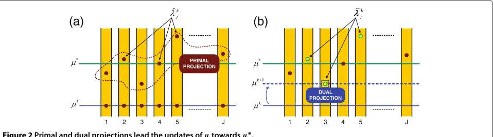
Figure 2a explains the effects of the three steps of the CDM graphically from the dual domain point of view. Each bar represents an entity (Jin total) and a point in that bar indicates the value of the dual variableλk_j orλˆk_j. The highest the point the highest the value. At the beginning of thekth iteration, the dual subproblems enforceλk_j =μk∀j

and translate these dual values to the primal variables in yk. Immediately after the primal projection, the corrected values inyˆkare converted again to dual variables, i.e.,{ˆλk_j}. In the figure, we appreciate the effect of the primal projec-tion on the Lagrange multipliers of interest. In short, we notice that (i) all values increase and (ii) there is at least one value belowμ∗.

The role of the dual projection in (14) is then to update toμk+1by selecting the closest value toμk from the list

{˘λk_j}, that is,μk+1 = min{˘λk_j}ifμk < μ∗, as depicted in Figure 2b. Together with the previous results, i.e.,λ˘k_j ≥μk andλ˘k_j ≤μ∗, the new update verifiesμk+1∈[μk,μ∗] and thus our initial hypothesis (μk < μ∗) is also satisfied for the next iteration unlessμk+1=μ∗. Therefore, successive iterations confirmμk k−→→∞ μ∗and, accordingly,yˆk k−→→∞ y∗_j ∀j. This concludes the proof of the proposed method.

4 Convergence rate analysis and stopping criterion

This section provides additional insights into the pro-posed CDM by means of the following particularization of (1),

min

{xj},y J

j=1fj(xj)

s.t. xj∈Xj, j=1,. . .,J

hj(xj)≤yj, j=1,. . .,J J

j=1yj≤C

y∈Y, Y=Y1×. . .×YJ

(19)

where the variables in{xj}as well as the subsets in{Xj}are uni-dimensional. To be precise, not all the problems that can be formulated as in (19) are considered in the follow-ing convergence analysis but only those with the followfollow-ing dependance between the primal variableyjand the dual variableλjin the subproblems of the CDM, still interest-ing as far as usual problems in the literature exhibit that relationship (see some examples in Section 5),

yj=aj

λj −α

+bj, for a certain value ofα >0,

aj>0 andbj∈R

(20)

In the general case, the relationship betweenyjandλj can be established again, thanks to the KKT optimality conditions of the problem. Therefore, let us construct the Lagrangian of (19), that is,

1 5 J

k

*

ˆk j

PRIMAL PROJECTION

(a)

(b)

k

*

1

k

DUAL PROJECTION

k j k

2 3 4 1 2 3 4 5 J

L({xj},y,{λj},μ,{ξj})= J

j=1fj(xj)+μ ( J

j=1yj−C)

+ J_j=1λjhj(xj)−yj

+ J_j=1ξT_j(g_j(xj))+ J

j=1ψ T jqj(yj)

(21)

and consider the following optimality condition,

∂L ∂xj = ˙

fj(xj)+λjh˙j(xj)+ξTj

∂ ∂xj

g_j(xj)=0 (22)

wheref˙ andh˙ stand for the first derivatives of the func-tionsf andh, respectively. Note that ifxj ∈/ bd Xjthen ξ_j=0due to complementary slackness and

λ_j= −f˙j(xj) ˙ hj(xj)

(23)

Moreover, if the constraint h(xj) ≤ yj is satisfied with equality (the usual case as we consider coupled problems) thenxj=h−_j 1(yj)and the relationship betweenλjandyjis established.

Finally, as we show in Section 5, (20) is found for com-mon functionsf andhappearing in usual problems. Fur-thermore, the convergence rate of the proposed method can be derived assuming (20) and a stopping criterion that enhances the performance of the CDM can be designed. These two issues are developed in the following subsec-tions.

4.1 Convergence rate analysis

In order to find out the convergence rate of the proposed method, let us compare the value of|(μk)−α−(μ∗)−α|in two successive iterations, i.e.,kandk+1. First, let us clas-sify the optimal primal variables{y∗_j}into three groups:I∗ includes the indexesjcorresponding to the variables that satisfyy∗_j = infYj,S∗embraces the indexes wherey∗_j = supYjand finally,A∗contains the remaining indexes, i.e., those associated toyj∈/bdYj. Using (20) and recalling the optimality conditionλ∗_j =μ∗seen in (11), it is true that

y∗_j =

⎧ ⎨ ⎩

aj(μ∗)−α+bj j∈A∗

mj j∈I∗

dj j∈S∗

(24)

where mj = infYj and dj = supYj. Assuming that J

j=1y∗j =Cis fulfilled, we get

μ∗−α= C−

j∈A∗bj−j∈I∗mj−j∈S∗dj

j∈A∗aj

(25)

For any other valueμk=μ∗we define

yk_j =

⎧ ⎨ ⎩

aj

μk−α+bj j∈Ak

mj j∈Ik

dj j∈Sk

(26)

where the subsetsAk,Ik, andSkare defined likewiseA∗, I∗_{, andS}∗_{but refer to the indexes of the variables in{y}k

j}. Let us assumeμk < μ∗and let us obtain{yk_j}from (26). Clearly, sinceμk−α > (μ∗)−α, it holds thatyk_j ≥y∗_j ∀j. As a result of the primal projection in (12), now with the objective value modified by the weighting matrixW = [ 1/a1,. . ., 1/aJ]T, i.e.,W1/2||yk − ˆyk||2, the correctedyˆk_j values can be expressed as

ˆ yk_j =

⎧ ⎨ ⎩

aj

μk−α+bj−ajK j∈Ak

mj j∈Ik

dj−ajK j∈Sk

(27)

for the value ofK > 0 to be determined. The proof is very similar to the caseW = Iin “Proof of Proposition 1” in Appendix and the convergence of the method is not affected. We use this projection in this particularized ver-sion simply because it offers better performance and we did not use it before just because we had no means to find a better weighting matrix than the identity matrix.

At the third step of the method, i.e., the dual subprob-lems, the reduced list{˘λk_j}is obtained from the valuesyˆk_j

in (27) withj∈Ak∪Sk. In other words, reversing (20) we find

˘ λk_j

−α

= yˆ

k j −bj

aj = ⎧ ⎨ ⎩

μk−α−K, ∀j∈Ak

dj−bj

aj −K, ∀j∈Sk

(28)

Finally, in the dual projection we select the minimum value in{˘λk_j}, which is in this case the closest toμkgiven μk < μ∗becauseμk+1∈[μk,μ∗] (see Section 3.3),

μk+1=min{˘λk_j} (29)

or equivalently,

μk+1

−α

=max{˘λk_j} =

μk

−α

−K (30)

since dj_aj−bj is always lower than μk−α or otherwise dj−bj

aj −Kwould belong toAk. Note in (27) that the defi-nition of the subsetsAk _andSk_impliesd

j < aj(μk)−α +

Using the previous results, we can state that

|μk+1

−α

−μ∗−α| = |

μk

−α

−μ∗−α−K| (31)

This can be further refined if K is developed using (27) andJ_j=1yˆk_j =C,

K=

μk−α_j∈Akaj+j∈Akbj+j∈Ikmj+j∈Skdj−C

j∈Ak_∪Skaj

=

j∈Akaj

j∈Ak_∪Skaj

μk−α−

j∈Akaj

j∈Ak_∪Skaj

×

C−_j∈Akbj−j∈Ikmj−j∈Skdj

j∈Akaj

(32)

Particularly, note that the expression within brackets in (32) is exactly(μ∗)−α when the subsetsAk, Ik andSk coincide with the optimal ones. We say that the algorithm is in theoptimal zonewhen the sets(Ak,Ik_,Sk_)coincide with(A∗,I∗,S∗).

Finally, we can conclude that the speed of convergence within the optimal zone obeys the following rule, which is obtained by plugging (32) into (31),

|(μk+1)−α−(μ∗)−α| = |(μk)−α−(μ∗)−α|

×

1−

j∈A∗aj

j∈A∗_∪S∗aj

(33)

In other words, (μk)−α converges linearly to (μ∗)−α except whenS∗ = {∅}, showing superlinear convergence. Alternatively, if the initial hypothesis isμ0> μ∗, the con-vergence is also linear expect forI∗ = {∅}, in which case it is superlinear. Note in both cases that since (1) and (19) are assumed coupled problems,A∗= {∅}.

4.2 Stopping criterion

The previous convergence rule in (33) can be used to define a stopping criterion for the CDM. It is based on the particular evolution followed byμkinside the optimal zone. For that purpose, let us take three consecutive val-ues ofμ, i.e.,μk,μk+1, andμk+2, all of them in the optimal zone. The successive application of (33) leads to

|(μk+l)−α−(μ∗)−α| = |(μk)−α−(μ∗)−α|

×

1−

j∈A∗aj

j∈A∗_∪S∗aj l

l= {0, 1, 2}

(34)

From (34) it is verified that

μk+2−α−μk+1−α

μk+1−α_−μk−α =1−

j∈A∗aj

j∈A∗∪S∗aj

(35)

and therefore, in the optimal zone, the left side of (35) is a constant number regardless ofk. From the practical point of view and thanks to this result, we can monitor the evolution of

SCk =

μk+2−α−μk+1−α

μk+1−α_−μk−α , ∀k (36)

and stop the iterations whenSCk stabilizes to a constant value. Afterwards, the optimal solution is readily obtained since at that point we know which allocations saturate to eithermjordjand the exact value ofμ∗can be computed by means of (25).

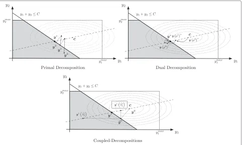
4.3 Graphical comparison among decomposition techniques

In the sequel, we include a graphical comparison among decomposition techniques and the goal is to highlight the manner in which the different methods operate in essence. We do this with the support of the following toy optimization problem

min

x1,x2,y1,y2 a1(x1−c1) 2_+a

2(x2−c2)2

xi≤yi, i=1, 2

s.t. y1+y2≤C

0≤xi≤xmaxi , i=1, 2 0≤yi≤xmaxi , i=1, 2

(37)

where we have included the variables yi to match the formulation of the proposed CDM and a primal decom-position as well. In Figure 3, we compare our proposed method to the classical decomposition techniques. In all the cases, the feasibility region of the problem in terms of the variablesy1,y2is marked in grey. Also, the contour lines of the objective function (centered atc =[c1,c2]T) are represented in the plots (even we know that the depen-dance of the objective function is on x1,x2 instead of

y1,y2).

Figure 3Comparison among decomposition techniques.Toy example.

and also betweenλjandμ. For that purpose, we consider again the Lagrangian of the problem, that is

L(x,y,λ,μ,ξ₁,ξ₂,ψ₁,ψ₂)

=a1(x1−c1)2+a2(x2−c2)2+λT(x−y)

+μ(y1+y2−C)

− 2_i=1ξ_1,ixi+ 2

i=1ξ1,i(xi−x max

i )

− 2_i=1ψ_1,iyi+ 2

i=1ψ1,i(yi−y max

i )

(38)

For the casexi ∈ (0,xmaxi ),i = 1, 2 andyi = xi, the dual variables inψ_i andξ_i satisfyψ_i = ξ_i = 0,i = 1, 2 due to slackness (note thatymax_i =xmax_i ,i=1, 2). In that con-ditions, the KKT optimality condition∂L/∂xi = 0 forces

xi=ci−

λi

ai

(39)

Furthermore, if we take into account thatyi = xi in the case of interest andλ_i = μ due to the KKT optimality condition∂L/∂yi=0, then we verify that

yi(μ)=ci−

μ ai

(40)

The dashed line in Figure 3 shows all the points that can be obtained by changing the value ofμin (40). Note in

particular that for μ = 0 the optimum of the uncon-strained version of (38) is achieved. Using the dual decom-position technique (in the figure we start withμ0=0), the successive updates move along this line (the orientation and module defined by the subgradient) until the optimal solution is achieved.

interesting feature of the proposed method in comparison with the other techniques, that is, the step is automatically controlled.

5 Applications and numerical results

In the sequel, we present three different applications of the proposed method, the first two are related to power allocation problems and the third one deals with DBA in satellite networks. In the first problem, a decentralized solution is required to reduce the amount of signaling information. In the second one, a centralized implemen-tation of the CDM is used to solve a time-varying water-filling problem and the aim is to show the benefits of having an unsupervised method in that changing con-ditions. Finally, the third example shows the advantages of the proposed technique when a small allocation time is required in order to accommodate a large number of users.

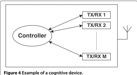
5.1 Decentralized power allocation for cognitive radios Let us consider a communication device that is able to establish simultaneous communication links by joining several networks or using multiple channels within the same system (e.g., this is possible in IEEE 802.11n). To do so, the device integrates multiple radio transceivers [23,24] which, at their turn, operate over multiple sub-channels or subcarriers in order to combat the multipath fading (see Figure 4). We assume that the device can sense the wireless channel and determine the non-used subcarriers in each subsystem, as it is usual in cogni-tive scenarios. Furthermore, each transceiver is able to optimally allocate the available power among its subcarri-ers using the water-filling solution. This is advantageous from the system design point of view because we can employ off-the-shelf radio transceivers and simply balance the device power among them. Finally, there is a central controller that performs the distribution task, being the global objective to maximize the total sum rate capacity. Note that, depending on the signal strength and capacity in each subsystem, some of the transceivers may remain temporarily idle.

Controller

TX/RX 1

TX/RX 2

TX/RX M

Figure 4Example of a cognitive device.

The problem can be formulated forMradio transceivers as

max

{Pi}

M

i=1ri(Pi)

s.t. M_i=1Pi≤PT

Pi≥0, i=1,. . .,M

(41)

whereri(Pi)is the transmission rate of theith transceiver when powerPi is allocated to it andPT is the total avail-able power. Each of the transmission rates is actually the result of another optimization problem, that is,

ri(Pi)= ⎧ ⎪ ⎪ ⎪ ⎪ ⎨ ⎪ ⎪ ⎪ ⎪ ⎩

max

{pi j}

Nsi

j=1BWilog

1+ p

i jHji N0BWi

s.t. pi_j≥0 Ni

s

j=1pij≤Pi

(42)

whereNi

sis the number of subcarriers of theith radio,BWi stands for subcarrier bandwidth, N0 is the noise power spectral density, and H_ji is the channel gain at the jth subcarrier of theith transceiver.

Note that given the separability of the problem, i.e., there are many independent transceivers coupled by a total power constraint, a decentralized optimization method is adequate both from a mathematical and a prac-tical point of view. In this approach, the controller decides the total power per transceiver and each subsystem com-putes its own optimal allocation. The application of the CDM to solve (41) is briefly detailed next.

Givenμk < μ∗, each transceiver computes the follow-ing dual subproblem,

max

{pi,j},Pki Ni

s

j=1BWilog

1+ _N0pi,j_BWiHi,j−μkP_ik

s.t. Nsi

j=1pi,j≤Pki

pi,j≥0

(43)

and the application of the KKT conditions gives the solution

pi,j=BWi

1

μk −

N0 Hi,j

+

P_ik=N

i s j=1pi,j

(44)

As a result of the dual subproblems we obtain Pk = [P₁k,. . .,P_Mk ]T and we use it as the input for the primal projection, that is,

min

{ˆPki}

|| ˆPk−Pk||2

s.t. M_i=1Pˆk_i =PT

ˆ Pk_i ≥0

(45)

wherePˆk =[Pˆ₁k,. . .,Pˆ_Mk ]T.

the optimal allocation by its own. As a result of the pri-mal subproblems, the Lagrange multipliers associated to

the constraints Nsi

j=1pi,j ≤ ˆPik at thekth iteration, i.e.,

ˆ

λk_i, are obtained. Discarding the values that result from

ˆ

P_ik=0, we obtain the reduced list{˘λk_i}and finally, the dual projection updatesμkfrom{˘λk_i}by doing

μk+1=min{˘λk_i} (46)

A completely different approach is to gather all the information at the controller and to compute there the optimal power allocation. Afterwards, the result is sent back to the transceivers. Note that this centralized solu-tion has an important drawback in terms of signaling because the powers in all the subcarriers and all the transceivers need to be exchanged. On the contrary, decentralized solutions benefit from transceiver-level sig-naling. In the numerical results below, we compare the CDM to other approaches.

5.1.1 Numerical results

We consider a device with three different OFDM trans-mitters. The first transmitter employs 256 subcarriers spanning a total bandwidth of 1.536 MHz (6 kHz per sub-channel), the second one has 256 subcarriers as well and 3.072 MHz of bandwidth (12 kHz per subchannel) and the third one manages 128 subcarriers in 1.28 MHz of band-width (10 kHz per subchannel), so that a total of 640 sub-carriers and 5.888 MHz have to be controlled (see Table 1). We assume frequency selective Rayleigh-fading channels in all three systems with a channel length of 20 taps and an exponential power delay profile where the delay spread is 1 ms. Mean channel gain is 0 dB in system 1,−10 dB in system 2, and −5 dB in system 3. Moreover, we assume that the noise power spectral density is flat over frequency withN0=σn2/BW1, beingBW1the subcarrier bandwidth in system 1. Initially, we set up a uniform power allocation in all the methods and the total available power is always

PT(dB)=σn2(dB)+10 log10(640)+5.

Figure 5 shows a multi-system water-filling allocation example. The plot at the top depicts one channel realiza-tion for the three systems whereas the plot at the bottom shows the optimal power allocation. As expected, most

Table 1 Description of the subsystems

Subsystem number

Number of subcarriers

Subcarrier bandwidth (BWi)

Subsystem bandwidth

1 256 6 kHz 1.536 MHz

2 256 12 kHz 3.072 MHz

3 128 10 kHz 1.28 MHz

f1 f1+0.76 f2 f2+1.02 f2+2.05 f3 f3+1.28

−40 −30 −20 −10 0

Frequency (MHz)

Gain (dB)

Subchannel gains

f1 f1+0.76 f2 0 f2+1.02 f2+2.05 f3 f3+1.28

0.5 1 1.5x 10

−3

Frequency (MHz)

PSD(W/Hz)/

σ n

2

Power allocation

Figure 5Distributed water-filling example.Top: channel gains. Bottom: power allocation. Inf1–f3 we have the initial band frequencies of subsystems 1–3.

of the power is allocated to transceivers 1 and 3, which are the ones that have the best channel condition. On the contrary, subsystem 2 only allocates power to a few subcarriers that have the highest channel gains. Notwith-standing, in absolute terms, transceiver 2 receives quite a large allocation in order to exploit the higher subcarrier bandwidth.

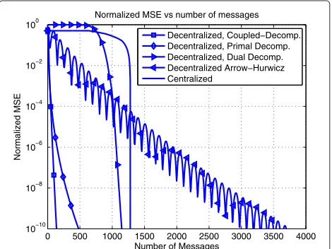
Figure 6 shows the evolution of the Normalized Mean Squared Error (NMSE) in the power allocation with respect to the number of messages exchanged between the transmission subsystems and the central controller. The optimal power allocation is computed using the bisec-tion method (relative error below 10−5). We compare the proposed CDM to the classical primal and dual decom-position techniques, the classical primal–dual algorithm of Arrow et al. [16] and also to a centralized approach. The classical decomposition techniques useαk = 1/√k

0 500 1000 1500 2000 2500 3000 3500 4000 10−10

10−8 10−6 10−4 10−2 100

Number of Messages

Normalized MSE

Normalized MSE vs number of messages

Decentralized, Coupled−Decomp. Decentralized, Primal Decomp. Decentralized, Dual Decomp. Decentralized Arrow−Hurwicz Centralized

as step-size and the Arrow–Hurwicz method initializes the value in the dual variableμto 0, the primal variables with a uniform power allocation and the step-size is fixed to 0.1. On the one hand, results show that the proposed CDM is the best option, whereas the remaining alterna-tives require at least to double the amount of signaling in order to achieve the same allocation error. On the other hand, note that the classical decomposition techniques as well as the primal–dual approach are penalized in terms of convergence speed even taking into account that we have manually adjusted the step-size of each method in order to achieve the best possible result. Finally, note also that a centralized approach is not efficient at all as far as the allocation error becomes small enough only when the entire allocation has been transmitted. This requires 640 messages in our case to send the channel gains to the controller and 640 messages more to return the optimal power allocation values to the radios.

5.2 Power allocation in a conventional OFDM transmission

In the following, we apply our method to a classical water-filling problem where a decentralized solution is not necessary. In this occasion, we are interested in the adaptability of the method in time-varying scenarios.

Let us consider the well-known single-user water-filling solution over parallel Gaussian channels ([25], Sec. 10.4), which provides the optimal power allocation to the sub-carriers of an OFDM-based system in order to maximize the mutual information given a total power constraint. Mathematically,

max

{pi}

Ns

i=1log

1+ _σpi2 ni

s.t. pi≥0 Ns i=1pi≤P

(47)

where Ns is the total number of subcarriers or paral-lel channels in the system, P is the total transmission power,σ_ni2 is the noise variance in theith subcarrier and

pistands for the allocated power. The application of the KKT optimality conditions to (47) leads to the solution

pi=

1 μ−σ

2 ni

+

(48)

where(a)+ = max{0,a}and _μ1 is denoted as the water-level and shall be chosen in order to satisfy the total power constraint. Typically, the bisection method is employed to find μ∗. However, note that (47) can be rewritten in the form of (2) and also (19). Therefore, we can apply the proposed CDM as well. Indeed, (48) and the relation-ship in (20) match if we identifypiwithyi andμwithλi (remember that the required relationship applies only to

yi∈/bdYi, that is,yi=pi>0).

5.2.1 Numerical results

Let us assume Ns = 512 subcarriers. The channel is time-varying and frequency selective; it has 20 taps. The power delay profile is assumed exponential with a delay spread of 1 ms and the baseband sampling time is 1μs. We compare now the proposed CDM to the bisection method and also to the classical primal–dual algorithm in [16]. It is remarkable that the CDM requires no modifi-cation at all (it is completely unsupervised) and the same holds for the primal–dual algorithm. On the contrary, the bisection method requires a slight modification to be able to track the time-varying scenario. For that purpose, we introduce the updating factorα_u. Initially, the method is applied as usual, that is, having the initial hypothesis onμ0_l andμ0_u(two values that are below and aboveμ∗, respec-tively), we computeμ1 = 1/2(μ0_l +μ0_u)and we update μ1_l toμ1 ifNs_i=1pi(μ1) > Por μ1_h toμ1 otherwise. In the subsequent iterations, given that the channel is time-varying, we need to check first ifμk_l andμk_hare still valid. IfNs_i=1pi(μk_l) >Pis not accomplished, we updateμk_l to

μk_l

αu and we repeat this while

Ns

i=1pi(μkl) >P. Similarly, if

Ns

i=1pi(μku) <Pis not attained, we modifyμkutoαu·μku and we repeat this whileNs_i=1pi(μku) <P. Then, we com-puteμk+1=1/2(μk_l +μk_u)and we update the hypothesis accordingly, as in the normal version of the technique.

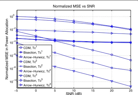
Figure 7 plots the NMSE of the power allocation for both methods as a function of the mean SNR. As in the previous application example, we compute the opti-mal power allocation using the bisection method (relative error below 10−5). Moreover, all the algorithms are ini-tialized to the optimal solution for the current channel condition, α_u = 1.05 in the bisection technique, the step-size is fixed to 0.001 in the Arrow–Hurwicz method and we have considered three different channel velocities,

−5 0 5 10 15 20 25

10−10 10−8 10−6 10−4 10−2 100

SNR (dB)

Normalized MSE in Power Allocation

Normalized MSE vs SNR

CDM, Tc1 Bisection, Tc1 Arrow−Hurwicz, Tc1 CDM, Tc2 Bisection, Tc2 Arrow−Hurwicz, Tc2 CDM, Tc3 Bisection, Tc3 Arrow−Hurwicz, Tc3

namely, (i)T_c1 = 10·TCDM, (ii)T_c2 = 100·TCDM, and (iii)T_c3 =1000·TCDM, whereTCDMis the time taken by one complete iteration of the CDM andTi

cis the coher-ence time of the channel at the ith scenario. Note that we have manually adjusted αu in the bisection method and the step-size in the primal–dual algorithm in order to achieve the best possible performance at the worst chan-nel condition, that is, when the chanchan-nel coherence time is the smallest one, i.e.,T_c1.

Results show that the CDM usually outperforms the bisection method and it is far better than the primal–dual algorithm. Indeed, it performs worse than the bisection only forT_c1and at low SNR. Note that since the CDM has no user-defined parameter, it automatically adapts to the different channel velocities. On the contrary, this adap-tation does not occur in the other two methods. This is reflected in Figure 7, where, for example, the bisection method saturates to an NMSE around 10−4 _forT1

c, Tc2, andT3

c as the SNR grows.

5.3 Fair DBA

The fair DBA problem arises in many-to-one communica-tion systems [26,27] and the goal is to fairly distribute the available bandwidth. In many cases and specially in sys-tems with a huge number of users [28], the computational cost of the techniques plays an important role. Addition-ally, let us remark that recent works on the topic aim at providing mechanisms for QoS differentiation [4,29] to modify a plain fair allocation. Therefore, we consider the following network utility maximization (NUM) formula-tion to solve a fair DBA problem,

max

{rj}

N

j=1Uj(rj;pj)

s.t. mj≤rj≤dj, j=1,. . .,N N

j=1rj≤B

, (49)

where B is the available bandwidth, rj is the rate allo-cated to thejth flow, andUjis thejth utility function (the terms bandwidth and rate are used interchangeably). The parametersmj,dj (with 0 ≤ mj < dj), and pj > 0 are used to define the QoS requirements for each ongoing connection and they represent the minimum necessary rate, the required (maximum) bandwidth and the prior-ity of thejth flow, respectively. Furthermore, we assume that _jmj < B < jdj, i.e., the problem is coupled. As argued before, the utility functions can adequately be chosen in order to achieve a fair distribution of resources in different degrees. The following family of functions parameterized byγ

Uj(rj;pj,γ )=

pjlog(rj), γ =1

pj r(j1−γ )

1−γ , γ =1

(50)

define different types of fairness, being γ → ∞(max– min fairness) andγ = 1 (proportional fairness) the most relevant ones [29].

Note that (49) can be rewritten in the form of (19) and in particular, the problem is strictly convex and we assume that strong duality holds, i.e., there is at least one strictly feasible point. Therefore, we can apply the KKT optimality conditions to solve (49) semi-analytically. In this case, the optimal rates must verifye

r_j∗(μ)=

pj

μ

1 γ

dj

mj

(51)

and the optimal value ofμis such thatN_j=1r∗_j(μ∗)= B. The bisection method is a classical technique widely used in the literature in order to approximateμ∗but, alterna-tively, we can also apply the enhanced version of the CDM. Specifically, by adding the new variables{yj}and identify-ingfj(rj)with−Uj(rj)andhj(rj) = rj, (23) together with

rj=h−j 1(yj), (51) turns into

yj=

pj

λj 1

γ

(52)

when mj < yj < dj and has the required form in (20). Therefore, once the subsetsS∗,I∗, andA∗are known, the optimal value ofμis readily found according to (25) as

μ∗=

i∈A∗√γ pi

B−_i∈I∗mi−i∈I∗di γ

. (53)

5.3.1 Numerical results

Let us draw the values ofmjfrom an integer uniform dis-tribution between 0 and 10. Each request djis obtained

summing mj and an integer random number between 0

and 100. The priority values pj are drawn from a uni-form distribution that takes values between 0.25 and 5 in steps of 0.25 and γ = 1. Figure 8 plots the mean allocation time, i.e., execution time, of the CDM when centrally computed in combination with the stopping cri-terion defined in Section 4.2. The algorithm has been executed in a Intel©Core 2 Duo CPU running at 2.2 GHz and programmed in Matlab©. We have considered three different values for the total available bandwidth, namely

B1 = _jmj+0.25jdj,B2 = jmj+0.5jdj, and

B3 = _jmj+0.75jdj. The results of the CDM have been compared to the classical bisection method and to the hypothesis testing method [30]. Since the allocation time is not sensitive to the available capacity for the latter methods, in Figure 8 we distinguish amongB1,B2, andB3 only for the CDM.

1 2 3 4 5 6 7 8 9 10 x 105 0

1 2 3 4 5 6

Number of Users (N)

Allocation Time (s)

Allocation Time vs Number of Users

CDM, B3 CDM, B2 CDM, B1 Hypothesis Testing Bisection

Figure 8Allocation time.

with respect to the optimal solution. The hypothesis test-ing strategy always achieves the exact optimal solution (see the details in [30]). The bisection method has been adjusted to achieve a relative error in the allocation lower than 10−6, or in other words,

||rBI−r∗|| ||r∗|| ≤10

−6_{, (54)}

wherer∗is the optimal allocation (which can be obtained with the hypothesis testing method) andrBIis the alloca-tion achieved by the bisecalloca-tion method. Initially, the two hypothesis for the values ofμare 0 and 10. In the CDM we stop the iterations when

|SCk+1−SCk| |SCk+1_| ≤10

−2_{. (55)}

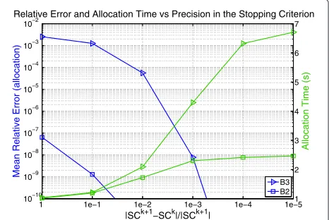
Note that as the number of users grows, the difference in time between the proposed method and the others also grows, specially when the system is more restricted in terms of capacity, i.e., for B1. In this case, the CDM is able to compute the allocation in half the time required by classical methods. In terms of accuracy in the solu-tion, (55) gives the exact optimal solution forB1,B2 and a relative allocation error lower than 10−4_{forB3. Overall,} the solution is good in practice; it is optimal in capacity-constrained scenarios and nearly optimal in less critical situations. In order to illustrate the selection of the thresh-old for the stopping criterion, we plot in Figure 9 the evolution of the relative error and allocation time as a function of the accuracy in the stopping criterion. Note that a threshold of 10−2provides a good trade-off between both performance metrics for the worst scenario, i.e., for

B3. Finally, if we consider a higher available bandwidth, e.g., 99% of the whole system demand, this threshold value keeps the allocation time small as inB3 at the expenses of a higher allocation error (around 5%). However, the accu-racy degradation appears only in this extreme case and it

is not critical in practice as far as all the users nearly reach their demands.

6 Conclusions and future work

This article has contributed with novel decomposition ideas that efficiently intertwine the classical primal and dual decomposition approaches in a single iteration of a new technique, called the CDM. It solves generic convex optimization problems that have one coupling constraint with the known advantages of decomposition-based approaches, that is, the implementation of decen-tralized solutions. However, it reduces the number of iterations by more than one order of magnitude with respect to the classical primal and dual decomposition solutions and furthermore, it is completely unsupervised, that is, there is no parameter that requires a manual adjustment. Moreover, when the problem is particu-larized (but still of interest), additional results regard-ing the convergence rate of the proposed technique are achieved and an stopping criterion that enhances the performance of the method (in terms of the number of iterations required to achieve the optimal solution) is derived.

The proposed method has been tested in three different problems, two dealing with power allocation in OFDM-based systems and a third one dealing with DBA. In the first two cases, the goal is to find the well-known water-filling solution in power. In one case, we benefit from a decentralized approach that suits the system architec-ture whereas in the other case, the proposed method is applied to a conventional OFDM transmission that deals with a time-varying channel. In both examples, we have compared our solution to other decomposition strate-gies and our approach performs significantly better than the available alternatives when a decentralized solution is required. In particular, our results show that the signal-ing requirements can be reduced at least by a factor 2.

1 1e−1 1e−2 1e−3 1e−4 1e−5

10−10 10−9 10−8 10−7 10−6 10−5 10−4 10−3 10−2

Relative Error and Allocation Time vs Precision in the Stopping Criterion

|SCk+1−SCk|/|SCk+1|

Mean Relative Error (allocation)

Allocation Time (s)

1 2 3 4 5 6 7

B3 B2