R E S E A R C H
Open Access
Low-frequency ambient noise generator with
application to automatic speaker classification
Ricardo Santana and Rosˆangela Coelho
*Abstract
A novel low-frequency 1/fambient noise generator using fractional statistics is proposed in this article. The noise samples are obtained by transformation functions performed on pseudo-random uniform sequences. The 1/f
spectrum representation achieved for the generated noise samples, shows that this proposition is very promising for the investigation of the low-frequency noise effect in signal processing techniques, devices and systems. It is also demonstrated that it can be useful to serve as background ambient noise in speaker classification applications.
Keywords: 1/fambient noise, Fractional Brownian noise, Low-frequency statistics, Speaker classification
Introduction
In the last decades, the presence of low-frequency or 1/f noise has been widely observed in such a variety of systems [1,2]. In particular, 1/f-spectra acoustic noise has been measured in ocean noise [3], music [4] and speech [5]. Noisy environments can severely degrade the performance of speech and speaker classification appli-cations [6-8]. These background noise sources can have different temporal and spectral statistics. Therefore, 1/f acoustic noise shall be considered to achieve robust signal processing techniques.
Noises are random processes described by the shape of its power spectral density (PSD). The PSD of noises [1,9] is defined by S(f) ≈ 1
fβ with 0 ≤ β ≤ 2. Generally, the PSD shape family is achieved by filtering Gaussian white noise (fgwn) sequences using digital finite impulse response (DFIR) filters and signal processing techniques [10-12]. However, the wide-sense stationary can only be measured for very long sample sequences. Mandelbrot and Van Ness [9] showed that the 1/f noise statistics can be accurately represented by the fractional Brownian motion (fBm). fBm is defined as a non-stationary stochas-tic process. Nevertheless, the shape of the PSD and theβ
exponent can be quasi-stationary if the observed time is short compared to the process life time [1,13]. And thus,
*Correspondence: [email protected].
Electrical Engineering Department, Acoustic Signal Processing Laboratory of the Military Institute of Engineering (IME), Rio de Janeiro, RJ 22290-270, Brazil
it enables the application of the estimation theory for 1/f processes [14,15].
1/f fractional noise has S(f) ∝ f1−2H, where 1/2 <
H < 1 is the Hurst parameter [16]. The H parameter is described by the slow-decaying rate of the auto-correlation function (ACF) of the noise samples. It rep-resents the low-frequency or scaling invariance degree of the fractional noises and it is frequently close to 1.
This article proposes the generation of 1/f ambient noise samples based on the fBm statistics. In the present approach, the 1/f spectral behavior is obtained from the ACFs of the noise samples generated by the fBm pro-cess. The 1/f ambient noise sample generation is based on transformation functions performed on uniform random sequences. These functions are defined by the successive random addition algorithm using the midpoint displace-ment (SRMD) technique [17]. In a previous study, these transformation functions were successfully evaluated for a low-frequency optical noise samples generation [18].
The solution presented for the SRMD algorithm to generate the 1/f acoustic noise samples, is also imple-mented in a high-speed field-programmable gate array (FPGA) Development Kit. Each noise output value is then pulse coded modulation (PCM) encoded/quantized and sampled at 8 KHz to produce the ambient noise levels. For the experiments, it is considered the real or natural 1/f Airport [19] and Airplane [20] ambient noises and also an artificial Pink [20] noise. The validation results
include the estimation of the main parameters or statis-tics (β exponent,H, mean (μ), variance (σ2) and Kurto-sis (K)), the PSD and the heavy-tail distribution (HTD) curves and the Bhattacharyya distance (Bd). These results
are obtained from the real and the generated noise sam-ples. For the experiments, 1/f sample sequences are also generated by filtering a Gaussian white noise using the Al-Alaoui transfer function [21]. Furthermore, the per-formance of the proposed 1/f acoustic ambient noise generation is evaluated for a speaker identification task considering different signal to noise ratio (SNR) values.
The rest of the article is organized as follows. Section “1/f fractional Brownian noise: an overview” gives an overview of the 1/f fractional Brownian noise and describes the SRMD technique. Section “Imple-mentation setup” introduces the imple“Imple-mentation setup of the proposed 1/f ambient noise generator. The main validation results are reported and discussed in Section “Validation results and discussion”. The speaker classification task and the related results are shown in Section “Speaker classification experiments”. Finally, Section “Conclusion” presents the main conclusions of this work.
1/ffractional Brownian noise: an overview
For any instant t > 0, XH(t) is a fractional random
function with Gaussian independent increments [9]. The fBm is known as the unique Gaussian H-self-similar with self-similarity parameter and stationary increments (sssi)
random process. The variance of the independent incre-ments is proportional to its time interval accordingly to
Var[XH(t2)−XH(t1)]∝ |t2−t1|2H (1)
for all instantst1andt2and,
1. XH(t)has stationary increments.
2. XH(0)=0andE[XH(t)]=0for any instantt.
3. XH(t)presents continuous sample paths.
In other words, its statistical characteristics hold for any time scale. Thus, for anyτ andr>0,
[XH(t+τ )−XH(t)] d
≈r−H[XH(t+rτ )−XH(t)] (2)
where ≈d means similar in distribution andr is the ran-dom process scaling factor. Note thatXH(t)is a Gaussian
process completely specified by its mean, variance, H parameter. The ACF of 1/f XH, i.e., 1/2<H<1 is
ρX(k)=
σX2
2 [(k+1)
2H−2|k|2H + |k−1|2H] (3)
fork ≥ 0 andρX(k) =ρX(−k)fork < 0. In the present proposition, the spectral density is derived from the ACF of the 1/ffBm noise samples defined in (3). This is ensured by the PSD and ACF exponents that are both related to the Hparameter.
16−bits PCM
16−bits D / A
Data Analysis
8 kHz 1/f noise samples
SRMD
Considering a time indextdefined at the interval [ 0, 1], the SRMD algorithm establishes that settingX(0)=0 and X(1)as a Gaussian random variable (RV) with zero-mean and varianceσ2then,
Var[X(1)−X(0)]=σ2. (4)
and
Var[X(t2)−X(t1)]= |t2−t1|σ2 (5)
for 0 ≤ t1 ≤ t2 ≤ 1. To achieve this property a random
offset displacement (Di) with zero-mean and variance
δi2 = 1/2−(i+1)σ2, must be added to the noise sample.
For example, theX(1/2)value is obtained by the interpo-lation ofX(0) andX(1)with varianceδ2/22H+1. Several iterations are then proceeded to compose a 1/f fBm noise sample sequence. In order to find stationary increments, after the midpoints interpolation, aDi of a certain
vari-ance, ∝ (rn)2H (ris the scaling factor), is applied to all points (time increments) and not just the midpoints. The maximum number of iterations is defined byN=2maxlevel wheremaxlevelis generally applied in the interval [0,16] [9]. The other SRMD inputs are the standard-deviation and theHparameter.
Implementation setup
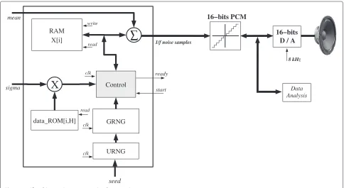
Figure 1 illustrates the experimental setup used for the demonstration of the proposed 1/f ambient noise gener-ator. The mean, variance and H values estimated from the real ambient and the artificial Pink noises are used as target parameters. The 1/f fBm noise generator is com-posed by the following main blocks: Uniform random number (URNG); Gaussian random number (GRNG); data ROM[i,H]; Control and X[i] RAM memory. The generation of the Gaussian RVs is based on transforma-tion functransforma-tions performed on Uniform variables using the Box-Muller method [22]. The Gaussian random number generator (GRNG) block provides the mean value for the Gauss(.)function.
Table 1βandHestimation results and theβestimation error
Noise β ε(β) H
Airplane (real) 1.13 0.124371 0.889
Airplane (proposed) 1.14 0.076390 0.890
Airplane (fgwn) 1.10 0.061164 0.862
Airport (real) 0.89 0.411874 0.882
Airport (proposed) 0.90 0.079132 0.891
Airport (fgwn) 0.81 0.076929 0.813
Pink (real) 1.02 0.041085 0.919
Pink (proposed) 1.01 0.065109 0.915
Pink (fgwn) 0.89 0.088994 0.847
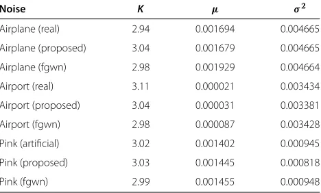
Table 2 Kurtosis, mean and variance statistics results
Noise K μ σ2
Airplane (real) 2.94 0.001694 0.004665
Airplane (proposed) 3.04 0.001679 0.004665
Airplane (fgwn) 2.98 0.001929 0.004664
Airport (real) 3.11 0.000021 0.003434
Airport (proposed) 3.04 0.000031 0.003381
Airport (fgwn) 2.98 0.000087 0.003428
Pink (artificial) 3.02 0.001402 0.000945
Pink (proposed) 3.03 0.001445 0.000818
Pink (fgwn) 2.99 0.001455 0.000948
The X[i] has i = 2maxlevel increments or noise levels. Uniform random number block was coded to produce 32-bit uniformly distributed samples with periodicity 1010. The linear feedback shift registers (LSFRs) are started by seed values to produce the pseudo-random sequences. The data ROM block performs the computation of the SRMD algorithm. The data ROM is indexed by i and H and it is defined by dataROM[i,H] := delta[sigmai] =
(12)iH
1 2
√
1−22H−2. The delta[i] values are stored and
addressed by the i andH indexes. This would be pro-hibitive due to the large amount of memory resources needs for storing a wide range of delta[i] values. However, Hvalues can be represented with only two-digits after the decimal point. Thus, 1,000Hvalues are necessary for each iteration of the SRMD algorithm. Since 0 ≤ maxlevel ≤ 16, delta[i] vector can have a maximum of 16,000 ele-ments. Hence, 1.6% of the ROM memory resource was needed to store the delta[i] vector. In fact, 1/f noises have 1/2<H<1 (close to 1) and hence the memory needs can be reduced. This second memory block is used to store the output sample vector (X[i]). The binary representation of eachX[i] noise output was truncated to 16-bit wide. The main functions of the control block are: Read the GRNG block output (Gaussian samples); Read the data ROM values according to the selected values indexed byiand H; Evaluate the delta by multiplying previous data ROM data to standard-deviation (sigma); Fill the initial values of theX[i] vector with the computed sigma∗Gauss values; Perform the loops iterations (one while and two for’s); Read fBm output noise sample levels from X[i] vector. The 1/f noise SRMD block implementation required ten digital signal processor (dsp) blocks and six phase locked
Table 3Bdresults
Noise Proposed fgwn
Airplane 0.0169 0.0663
Airport 0.0209 0.0969
loop (PLL) used for clock generation to achieve the target noise sample output rate. Following, each noise output value is PCM encoded/quantized and sampled at 8 KHz to produce the ambient noise levels. This sampling rate is necessary for the speaker classification experiments.
Besides the real ambient noises and the artificial Pink noise, samples obtained by filtering a Gaussian white noise are considered for the validation of the proposed method. The applied method uses the Al-Alaoui digital integrator transfer function [21] withβ/2 as the fractional order exponent to compose the transfer function H(z),
H(z)=
7T 8
(1+z−1/7) (1−z−1)
β/2
, (6)
whereT is the sampling period. The filter coefficients are obtained by the convolutionh(k) = a(k)∗b(k), where a(k)andb(k)are the firstN/2 terms obtained by expand-ing, respectively, the numerator and denominator of (6) in power series [12].
Validation results and discussion βandHestimation results
The β exponent is estimated from the linear regression applied to the PSD function curves. Table 1 shows the
β exponent, the mean square error (MSE) of theβ esti-mation, and the H results obtained from the real and artificial noises, and from the noise samples generated by the proposed and the fgwn methods. The results are presented for 320,000 samples since this is the size of the real ambient noise sequences. For theH estimation it is used the wavelet-based method [23] with 12 Daubechies filters and the 4–12 scale range. It can be seen that theβ
exponent values of the noise samples obtained from the proposed method, are very close to the values of the real ambient noises.
It can be noted that for the artificial Pink noise samples, the proposed and fgwn methods achieve quite similarH target values, i.e., the low-frequency statistics. However, theHresults estimated from the noise samples generated by the proposed method, are much closer to theHvalues of real ambient noises.
100 400 1000 4000
Frequency [Hz]
-40 -30 -20
S(f) [dBm/Hz]
Airplane (real) Airplane (proposed) Airplane (white filtered)
100 400 1000 4000
Frequency [Hz]
-50 -40 -30
S(f) [dBm/Hz]
Airport (real) Airport (proposed) Airport (white filtered)
(a)
(b)
(c)
Kurtosis, mean, variance statistics
Kurtosis measures the skewness of a sample from a Gaussian distribution. The K, mean and variance esti-mation results of the noise sequences are presented in Table 2. As expected, theKvalues are close to 3. Thus con-firming that the noise samples are Gaussian distributed.
Bhattacharyya distance
The Bhattacharyya distance measures the separability between two sample sequences with Gaussian distribution and is defined by
Bd=
1 2ln
|Ci+Cj| 2 |Ci|1/2|Cj|1/2
+ 1
8(μi−μj)
T
Ci+Cj
2
−1
(μi−μj) (7)
where μi is the mean vector and Ci is the covariance
matrix of classi=1, 2. TheBdare measured between the
generated sequences and the corresponding Airplane, Air-port and Pink noises. It can be seen from Table 3 the Pink
noise samples distribution produced by both methods, is very similar to the distribution of the artificial Pink noise. However, the samples distribution obtained from the pro-posed method are much similar to the distribution of the real ambient noises.
PSD results
The power spectral densities obtained from the real and the generated 1/f acoustic noise samples are pre-sented in Figure 2. The PSDs were measured using a high-performance 300 MHz bandwidth spectrum ana-lyzer. These results demonstrate the slow-decaying (3 dB/octave) behavior of the PSD shape of the 1/f noises. It can also be seen that the proposed method better represents the PSD behavior of the real acoustic noises.
HTD results
Figure 3 illustrates the HTD (P[X > x]) curves of the Airplane, Airport and Pink noise samples achieved by the proposed and fgwn methods. The HTD curves obtained from the real and the proposed method demonstrate that
they exhibit very close tails. This also confirms the H results (see Table 1) obtained from the proposed solution.
Speaker classification experiments
In a speaker identification process, a speech utterance has to be identified as to which of the registered speak-ers it belongs. For the experiments, the speech utterances were corrupted with the real and generated noise sam-ples. For the speaker identification were considered the mel-cepstral coefficients (MFCC) and the Gaussian mixed model (GMM) [24] which are respectively, the most com-monly used speech features and classifier employed in speaker recognition tasks.
A mixture of Gaussian probability densities is a weighted sum ofMdensities, and is given by
p(x|λ)=
M
i=1
pibi(x) (8)
where x is a random vector of dimensionD, bi(x), i =
1,. . .,M, are the Gaussian density components, and pi,
i=1,. . .,M, are the mixture weights.
Each component density is aDvariate Gaussian func-tion of the form
bi(x)=
e
−1
2(x− μ)TKi−1(x− μ) (2π )D2√|Ki|
(9)
with mean vectorμi and covariance matrixKi, whereT
denotes the transpose operation and |.| is the determi-nant. The GMM (λ) is parametrized by the mean vectors, covariance matrices, and mixture weights. The model parameters are estimated for a set of training data as the ones that maximize the likelihood of the GMM. The expectation-maximization (EM) algorithm [24] is used for the model parameters estimates. Considering a sequence ofT independent training vectorsX = {x1,. . .,xT}, the
normalized log-likelihood of the GMM is
logp(X|λ)= 1
T
T
t=1
logp(xt|λ). (10)
The decision rule of the speaker identification system chooses the speaker model for which this value is maxi-mum.
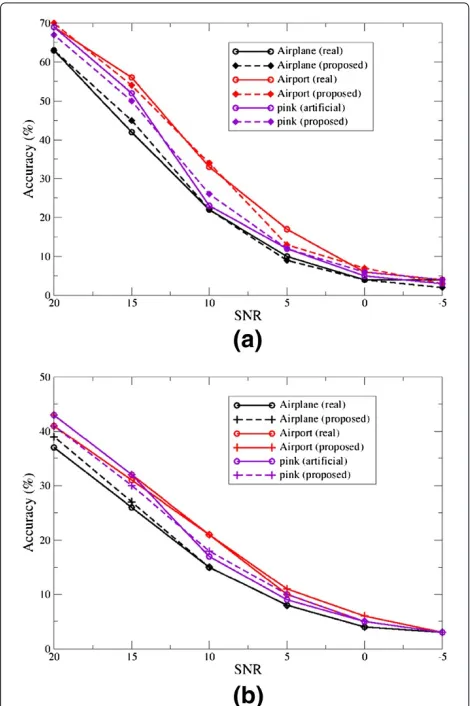
Speaker identification accuracy results
The speaker identification task evaluation is performed on the KING speech corpus. This is composed of conversa-tional sessions of speech recorded by 49 male speakers. For the experiments, five sessions are used resulting in 100 s average of speech per speaker, after silence removal. Three of these sessions (60s) are applied for the speaker model training. The remaining two sessions (40s), are used to evaluate the identification accuracies.
The speaker classification results are presented for test duration of 5 and 1 s. The real and generated 1/f noise samples are added to the speech utterances serving as background ambient noise. For the investigation, it is also considered the SNR 0 dB, 5 dB, 10 dB, 15 dB, and 20 dB to evaluate the system under different noisy conditions. For the identification task it was considered speech fea-ture vectors with 25 MFCCs, extracted from 20 ms speech frames, and M = 32 GMM components. The speaker identification accuracies are shown in Figure 4. The results show that the generated 1/f noise produced similar effect when compared to the real ambient noise. This means that it could be applied as artificial background noise.
Conclusion
A new low-frequency 1/f ambient noise generator using fractional statistics is described in this article. The PSD shape of the 1/f generated noise samples is achieved from the ACFs of the noise samples generated with the fBm process. The implementation of the 1/f ambient noise
generator enables the validation of the pattern and the PSD representation. It is shown that this proposition is very promising for the investigation of this noise effect in the signal processing techniques. Furthermore, the speaker identification experiments demonstrate that the generated ambient noise samples can be useful to serve as background or additive noise.
Competing interests
The authors declare that they have no competing interests.
Acknowledgements
This work is partially supported by the National Council for Scientific and Technological Development (CNPq) under the research grant 472461/2009-5.
Received: 20 May 2011 Accepted: 22 June 2012 Published: 17 August 2012
References
1. M Keshner, 1/f noise. Proc. IEEE.70, 212–218 (1982) 2. F Hooge, 1/f noise. Physica B+.C83, 14–23 (1976)
3. A Derzjavin, A Semenov, Ocean ambient low frequency acoustic noise structure in shallow and deep water regions. Journal de Physique IV.4, 1269–1272 (1994)
4. R Voss, J Clarke, 1/f noise in music: Music from 1/f noise. J. Acoust. Soc. Am.63(1), 258–263 (1978)
5. R Voss, J Clarke, 1/f noise in music and speech. Nature.258, 317–318 (1975)
6. Y Gong, Speech recognition in noisy environments: a survey. Speech Commun.16, 261–291 (1995)
7. J Ming, T Hazen, J Glass, D Reynolds, Robust speaker recognition in noisy conditions. IEEE Trans. Audio Speech Lang. Process.15, 1711–1723 (2007) 8. L Z˜ao, R Coelho, Colored noise based multicondition training technique
for robust speaker identification. IEEE Signal Process. Lett.18, 675–678 (2011)
9. B Mandelbrot, J Van Ness, Fractional brownian motions, fractional noises and applications. SIAM Rev.10, 422–437 (1968)
10. M Deriche, A Tewfik, Signal modeling with filtered discrete fractional noise processes. IEEE Trans. Signal Process.41(9), 2839–2849 (1993) 11. C Tseng, S Pei, S Hsia, Computation of fractional derivatives using fourier
transform and digital fir differentiator. Signal Process.80(1), 151–159 (2000)
12. Y Ferdi, A Taleb-Ahmed, M Lakehal, Efficient generation of 1/fβnoise
using signal modeling techniques. IEEE Trans. Circ. Syst.55, 1704–1710 (2008)
13. F Hooge, Discussions of recent experiments on 1/f noise. Physics.60, 130–144 (1972)
14. S Yousefi, J Jald´en, T Eriksson, Linear prediction of discrete-time 1/f processes. Signal Process. Lett.17(11), 901–904 (2010)
15. B Ninness, Estimation of 1/f noise. IEEE Trans. Inf. Theory.44, 32–46 (1998) 16. E Hurst, Methods of using long–term storage in reservoirs. Proc. Inst Civil
Eng, 519–543 (1956 )
17. M Barnsley, R Devaney, B Mandelbrot, H Peitgen, D Saupe, R Voss,The Science of Fractal Images. (New York, USA: Springer-Verlag, 1988) 18. L Z˜ao, R Coelho, Low-frequency optical noise generator using fractional
statistics. Electron Lett.46, 1072–1074 (2010)
19. FreeSFX, Airport ext busy tarmac, Ambiences/Background Sound Effects. [http://www.freesfx.co.uk/soundeffects/airports/]; 2009
20. A Varga, H Steeneken, M Tomlinson, M Jones, The noisex-92 study on the effect of additive noise on automatic speech recognition. Technical Report of Defence Evaluation and Research Agency [http://spib.rice.edu/ spib/1992]
21. M Al-Alaoui, Novel digital integrator and differentiator. Electron. Lett.29, 376–378 (1993)
22. G Box, M Muller, A note on the generation of random normal deviates. Ann. Math. Stat.29, 610–611 (1958)
23. P Flandrin, Wavelet analysis and synthesis of fractional brownian motion. IEEE Trans. Inf. Theory.38, 910–917 (1992)
24. D Reynolds, R Rose, Robust text-independent speaker identification using gaussian mixture speaker models. IEEE Trans. Speech Audio Process.3, 72–83 (1995)
doi:10.1186/1687-6180-2012-175
Cite this article as:Santana and Coelho:Low-frequency ambient noise gen-erator with application to automatic speaker classification.EURASIP Journal on Advances in Signal Processing20122012:175.
Submit your manuscript to a
journal and benefi t from:
7Convenient online submission 7Rigorous peer review
7Immediate publication on acceptance 7Open access: articles freely available online 7High visibility within the fi eld
7Retaining the copyright to your article

![Figure 3 illustrates the HTD (P[ X > x]) curves of theAirplane, Airport and Pink noise samples achieved by theproposed and fgwn methods](https://thumb-us.123doks.com/thumbv2/123dok_us/1138945.1142882/5.595.58.542.351.713/figure-illustrates-theairplane-airport-samples-achieved-theproposed-methods.webp)