Markets and Microstructure
Thesis by
Thomas Gorden Ruchti
In Partial Fulfillment of the Requirements
for the Degree of
Doctor of Philosophy
California Institute of Technology
Pasadena, California
2013
c
2013
Thomas Gorden Ruchti
Most of all to my advisers, Matt, Ben, Jakˇsa, and John. To Harold for getting me into this
Acknowledgments
I am especially grateful to Jakˇsa Cvitani´c, Ben Gillen, John Ledyard, and Matt Shum for
encouragement and guidance. For helpful discussion and advice, I also thank Shmuel Baruch,
Jonathan Brogaard, Andrea Kanady Bui, Claude Courbois, Federico Echenique, Jean
Ens-minger, Peter Foley, Gustav Haitz, Andrei Kirilenko, J. Morgan Kousser, Arseniy Kukanov,
Sangmok Lee, Emiliano Pagnotta, Jean-Laurent Rosenthal, and J. Andrew Sinclair. For
Abstract
This document contains three papers examining the microstructure of financial interaction
in development and market settings. I first examine the industrial organization of financial
exchanges, specifically limit order markets. In this section, I perform a case study of Google
stock surrounding a surprising earnings announcement in the 3rd quarter of 2009,
uncover-ing parameters that describe information flows and liquidity provision. I then explore the
disbursement process for community-driven development projects. This section is game
theo-retic in nature, using a novel three-player ultimatum structure. I finally develop econometric
tools to simulate equilibrium and identify equilibrium models in limit order markets.
In chapter two, I estimate an equilibrium model using limit order data, finding parameters
that describe information and liquidity preferences for trading. As a case study, I estimate
the model for Google stock surrounding an unexpected good-news earnings announcement
in the 3rd quarter of 2009. I find a substantial decrease in asymmetric information prior to
the earnings announcement. I also simulate counterfactual dealer markets and find
empiri-cal evidence that limit order markets perform more efficiently than do their dealer market
counterparts.
In chapter three, I examine Community-Driven Development. Community-Driven
De-velopment is considered a tool empowering communities to develop their own aid projects.
While evidence has been mixed as to the effectiveness of CDD in achieving disbursement
to intended beneficiaries, the literature maintains that local elites generally take control of
most programs. I present a three player ultimatum game which describes a potential
de-centralized aid procurement process. Players successively split a dollar in aid money, and
the final player–the targeted community member–decides between whistle blowing or not.
targeted recipients. My results describe a perverse possibility in the decentralized aid process
which could make detection of elite capture more difficult than previously considered. These
processes may reconcile recent empirical work claiming effectiveness of the decentralized aid
process with case studies which claim otherwise.
In chapter four, I develop in more depth the empirical and computational means to
estimate model parameters in the case study in chapter two. I describe the liquidity supplier
problem and equilibrium among those suppliers. I then outline the analytical forms for
computing certainty-equivalent utilities for the informed trader. Following this, I describe
a recursive algorithm which facilitates computing equilibrium in supply curves. Finally, I
outline implementation of the Method of Simulated Moments in this context, focusing on
Contents
Acknowledgments iv
Abstract v
1 Introduction 1
1.1 Chapter 2: Beyond the Bid-Ask Spread . . . 2
1.2 Chapter 3: Corruption and CDD . . . 3
1.3 Chapter 4: Econometrics and Computation . . . 3
2 Beyond the Bid-Ask Spread: Estimating an Equilibrium Model of Limit Order Markets 6 2.1 Introduction . . . 6
2.2 Literature Review . . . 8
2.3 Model . . . 11
2.3.1 Notation . . . 12
2.3.2 Dynamic Programming Characterization of the Limit Order Book . . 13
2.3.3 Risk Averse Active Trader . . . 14
2.3.4 Liquidity Suppliers and the Optimal Supply Problem . . . 18
2.4 Estimation . . . 19
2.4.1 Solving for Equilibrium . . . 20
2.4.2 Indirect Inference . . . 21
2.5 Empirical Results: A Snapshot of Google, October 14-16, 2009 . . . 22
2.5.1 Earnings Announcements, Asymmetric Information . . . 22
2.5.3 Informedness Ratio . . . 26
2.6 Robustness Checks: Levels of Competition . . . 28
2.6.1 Comparison of Fit . . . 28
2.6.2 Comparing Limit Order Markets and Dealer Markets . . . 30
2.6.3 Counterfactual Utilities . . . 31
2.7 Conclusion . . . 34
3 Corruption and Community-Driven Development 35 3.1 Introduction . . . 35
3.2 Model . . . 39
3.2.1 Splitting a Dollar in Aid . . . 39
3.2.2 Equilibrium Existence . . . 41
3.3 Relative patience and comparative statics . . . 44
3.3.1 Village patience and whistle blowing . . . 44
3.4 Conclusion . . . 46
3.5 Appendix . . . 47
3.5.1 V - Village . . . 47
3.5.2 C - Committee . . . 48
3.5.3 D - District . . . 49
3.5.4 Proof of Theorem 1 . . . 50
3.5.5 Comparative Statics . . . 52
4 Econometrics and Computation in Market Microstructure Models 54 4.1 Introduction . . . 54
4.1.1 Price Evolution surrounding EA by Google . . . 55
4.2 Liquidity Suppliers and the Optimal Supply Problem . . . 55
4.3 Counterfactual Utilities . . . 58
4.4 Solving for Equilibrium, detail . . . 61
List of Figures
2.1 Inference and Continuous Solution . . . 16
2.2 Inference and Interior Solution . . . 18
2.3 Inference and Boundary Solution . . . 19
2.4 Indirect Inference . . . 20
2.5 Bid-Ask Spread and Depth . . . 26
2.6 Informedness Ratio . . . 28
4.1 October 14, 2009 NASDAQ Totalview-ITCH feed . . . 55
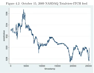
4.2 October 15, 2009 NASDAQ Totalview-ITCH feed . . . 56
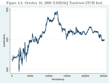
4.3 October 16, 2009 NASDAQ Totalview-ITCH feed . . . 57
List of Tables
2.1 Model Parameters . . . 12
2.2 Earnings Announcement Results . . . 25
2.3 Robustness Checks . . . 29
2.4 Counterfactual Profits and Utilities . . . 33
Chapter 1
Introduction
Since the 1990s, there have been many changes to equities markets and to development aid
practices. Historically, equities markets were once centralized, relying on specialists in the
New York Stock Exchange, and market makers on NASDAQ, to intermediate the market.
Similarly, the World Bank and related donors have carried out aid projects using top-down
strategies. Projects were developed, funded, and implemented under donor or World Bank
direction. However, mainstay exchanges have fractured, with liquidity going to other
ex-changes, internalizers, and dark pools (Duffie (2012)), while exchanges are computer-driven
more than ever. Community-Driven Development now accounts for a large portion of aid,
offering project development and implementation choices to in-need communities themselves
(Lessmann and Markwardt (2010)). The 1990s saw decentralization take hold in many
de-velopment practices and nearly all financial markets. In this thesis, I develop microeconomic
and econometric theory to explain interesting patterns in data concerning Community-Driven
Development and modern exchanges. In chapter 2, I quantify information asymmetry and
efficiency in modern limit order markets. In chapter 3, I set up a three-person ultimatum
game and find equilibrium that explains interesting outcomes in decentralized development.
In chapter 4, I develop the computational and econometric tools which are necessary for
1.1
Chapter 2: Beyond the Bid-Ask Spread
In this chapter I explore the microstructure of limit order markets empirically. Empirical
market microstructure has remained primarily in reduced form estimation. Contrasting
with previous studies, I fit parameters using an equilibrium model and explore the industrial
organization of these markets. Through a novel inference method, as outlined in Chapter
4, I quantify anticipated information flow and efficiency in a market for a single asset.
Information flow is in terms of new information about the asset’s underlying value. Efficiency
is characterized as the level of hedging need of traders that the market meets.
I empoy my methodology with a case study involving Google stock surrounding an
earn-ings announcement in the third quarter of 2009. I evaluate typical asymmetry measures,
specifically depth of book and bid-ask spread. To better communicate my own estimation
results, I develop a volume-insensitive measure of information flow into the market, the
In-formedness Ratio. The Informedness Ratio is defined as the ratio of volatility of the asset’s
true value from the perspective of the market and the perspective of some better-informed
trader. A higher number relates to higher asymmetry, which is found at the beginning and
the end of the trading day. As a robustness check, the interday levels of the Informedness
Ratio appear to fall following the earnings announcement, similar to the bid-ask spread.
I also look at efficiency in the market for Google surrounding the earnings announcement.
Employing the structural nature of the model, I can vary model parameters and simulate
data to match it. I vary the number of effective liquidity suppliers in the market at any
one point of time–essentially changing the market structure. From this simulated data, I
compute certainty-equivalent utilites for traders and better-informed traders to illustrate,
as one would expect, that more competition in the market results in higher efficiency. The
model fits for various numbers of effective liquidity providers is also found, and I find that
the model fits markedly better with a larger number of liquidity providers than two. Two
liquidity providers may illustrate a duopolist setting, and so we argue that the market for
1.2
Chapter 3: Corruption and CDD
I use microeconomic theory to further our understanding of corruption and development.
Development on the whole is understood to attract corruption. Community-Driven
De-velopment, a newer aid implementation, was designed to reduce corruption, and empower
communities to develop their own aid projects. I argue that the way we think about
corrup-tion in development, and specifically Community-Driven Development, may not be accurate.
Classically, considering corruption in a Becker and Stigler (1974) framework, a third party to
corruption serves as deterrent factor. However, such third parties are difficult to characterize
in many aid settings, and incentives facing those perpetrating graft lead corrupt individuals
to choose projects which may best hide their corrupt dealings (Shleifer and Vishny (1993)).
In a tradition of three-person ultimatum games, I present a new three player ultimatum
game which describes a potential decentralized aid procurement process. Players successively
split a dollar in aid money, and the final player–the targeted community member–decides
between whistle blowing or not. I feel as though this setting may more accurately describe
the settings as faced by project implementers as well as village members. The key feature
exploited here is that of a less engaged monitoring entity. The comparative statics I find
lend some light to possible directions for theoretical as well as empirical research into the
economics of decentralized aid and corruption in a decentralized setting.
1.3
Chapter 4: Econometrics and Computation
In my concluding chapter, I develop in more depth the empirical and computational means
to estimate model parameters in the case study in Chapter 2. While the setting I apply these
techniques to is specifically market microstructure and in particular, limit order markets, the
applications for such methods are wider in scope. Competition in supply curves is a notion
explored in auctions and other parts of industrial organization. Similarly, the econometric
however the way I implement them is different than previously explored.
I set up the model I use for estimating equilibrium trading in limit order markets. While
this analysis leaves out many of the details of the competing liquidity suppliers problem in a
discrete-price order book, the equilibrium concepts are standard. I first describe the liquidity
supplier problem, incorporating the discrete-price first-order and boundary conditions for the
informed active trader. I also find the equilibrium conditions among these suppliers.
I also develop computational tools to find efficiency in the market for an asset. These
utilities are used when analyzing simulated data from varying numbers of effective liquidity
suppliers in my paper. However, the structural methodology allows for any number of
parametric changes, from trader risk-aversion to the volatility of the asset’s underlying value.
The most important methodological piece to analysis of limit order markets is the method
of computing equilibrium in supply curves in a discrete-price setting. Following Baruch
(2008), it is possible to find a partial differential equation which characterizes equilibrium
supply in a continuous-price setting. However, in discrete prices, the equilibrium problem
be-comes more difficult, and analytially intractable. To circumnavigate ths difficulty, I develop
a recursive algorithm which facilitates computation of equilibrium supply curves. The
recur-sive algorithm employs some key features of limit order markets–any market with competing
suppliers, for that matter–and allows for implementation of standard dynamic programming
numerical methods.
The particular nature of limit order data lends itself well to time-series analysis, but
the limited depth in order books (ticks beyond the bid-ask spread), and the decreasing
importance of this depth, reduces the applicability of some standard panel asymptotics.
Because the analytical forms of my equilibrium supply curves are not available, I turn to
the method of simulated moments. Beyond that, the method of simulated moments requires
the use of a pseudo model to avoid the intractable equilibrium supply curves, and produce
moments. I use Indirect Inference to match the pseudo model from data to the pseudo model
an option because each instance of the order book lacks panel characteristics necessary for
asymptotic results. I therefore employ the time-series nature of the data, assuming that a
single equilibrium is played over a short period of time, and use in-fill asymptotics to achieve
consistency of my estimator. I then use several instances of the order book to achieve
over-identifying restrictions. By limiting the number of ticks of the order book that are considered
Chapter 2
Beyond the Bid-Ask Spread:
Estimating an Equilibrium Model of
Limit Order Markets
2.1
Introduction
In this paper, I study equilibrium trading in limit order markets. Limit order markets are
widely used in financial exchanges around the world, including New York Stock Exchange,
NASDAQ, Stockholm Stock Exchange, and Paris Bourse, among others. A limit order
mar-ket allows for direct interaction between traders, without a marmar-ket-making dealer. Traders
choose between market orders–which execute against existing orders in the book–and limit
orders–which enter the book with a limit number of shares and limit price and await
execu-tion with a market order. Despite widespread use, empirical studies of limit order markets
have been hampered by data availability and complexity of existing models. This paper
pushes forward the empirical analysis of these markets by specifying and estimating a
struc-tural econometric model of equilibrium trading in a limit order market. As a case study,
I estimate this model on the limit order book for Google stock surrounding a surprisingly
good earnings announcement in the 3rd quarter of 2009.
I develop an econometric framework based on work of Bernhardt and Hughson (1997)
and Biais, Martimort, and Rochet (2003), in which the authors study a model of imperfect
incorporates an insight by Baruch (2008), a paper subsumed by Back and Baruch (2012),
that liquidity suppliers’ choice of supply schedules can be recursively characterized as a
dynamic programming problem. This insight is key to my econometric procedure, allowing
me to apply tools and methodologies developed for estimating dynamic optimization models
to the explicitly non-dynamic (static) model of equilibrium in limit order markets. To my
knowledge, this is the first paper performing structural econometric analysis in such a setting.
I use this econometric framework to address two important questions. First, is
informa-tion transmitted evenly and quickly across the market? I present a measure of informainforma-tion
asymmetry, the Informedness Ratio. A higher ratio means that insiders have more
infor-mation than the market, with a lower ratio meaning asymmetry is less. The informedness
ratio is high a day before the examined earnings announcement, settling at a lower level the
day of the announcement, and continuing to fall the day after. The fall in the informedness
ratio the day of the announcement indicates information asymmetry and uncertainty fall
before the announcement is made. Second, what are the welfare implications of the switch
from dealer to limit order markets, pervasive in real-world financial markets? I simulate
counterfactual dealer markets using real data, and show that limit order markets perform as
well as, if not much better than, one would expect dealer markets to perform.
I address an important question in the microstructure literature involving pervasive
change in modern exchanges to a limit order-based system. Historically in most markets,
trade was handled by a single monopolist dealer. If a trader wanted to buy or sell a certain
number of shares, a dealer would quote terms, and the trade could be executed. Now most
exchanges use a limit order book. Traders have the option of placing market orders, which
execute against existing shares in the book, or placing a limit order, with a limit price and
quantity, which enters the book and waits for a market order to execute against it. I use
counterfactual examples to assess the change in market performance moving from two
deal-ers to the imperfect competition found in limit order markets. Arguments could be made
increasing welfare.1 However, a dealer could bring a level of expertise to an asset, allowing
a dealer to facilitate the market in times that decentralized traders would be unwilling to
make a market for an asset. Using my model, I simulate counterfactual dealer markets from
the data. Not surprisingly, more liquidity suppliers leads to higher welfare. As a robustness
check, I find the model fits better with five liquidity suppliers than it does with two or ten–
when traditional markets typically had one, but no more than two, dealers per asset. This
means that the market behaves effectively as if it has five dealers. More dealers
unambigu-ously means higher welfare, hence I conclude that limit order markets are more efficient than
a counterfactual dealer market would be.
I touch on several different literatures related to this work in section 2.2. Section 2.3
explains the limit order book as a dynamic program and the risk-averse active trader setting
used here. Section 2.4 discusses methods of simulation and estimation. I discuss my results
on earnings announcements in section 2.5. In section 2.6, I perform robustness checks of the
model specification and conduct an analysis of the move from dealer markets to limit order
markets. Section 2.7 concludes.
2.2
Literature Review
I take an equilibrium model of imperfect competition in a common value setting from
Bern-hardt and Hughson (1997), which is further analyzed for equilibrium in Biais, Martimort,
and Rochet (2003)2 and apply it in an empirical setting. Their analysis involves strategic risk-neutral liquidity suppliers competing in schedules for the business of a risk-averse agent
who is privately informed about the value of the asset and about hedging needs in a
com-mon value setting. Biais et al. extend previous analyses concerning what creates the bid-ask
spread, patterns in trading volumes, and oligopolistic incentives.3
1See Biais, Foucault, and Salani´e (1998).
2Madhavan (1992) uses the same risk-averse trader setting, but assumes competitive liquidity suppliers.
For a recent model on imperfect competition in a contrastingprivatevalue setting, see Vives (2011).
3See Kyle (1985) for the seminal batch-trading model, Glosten (1989) for the monopolist dealer problem,
Baruch (2008) makes a key analytical insight, by applying dynamic programming
meth-ods to analyze the same model. From an econometric point of view, this insight proves useful
in making these models amenable to estimation. While dynamic programming methods are
inherently valuable to a variety of problems in structural analysis, these methods are often
employed in explicitly dynamic models, where agents make intertemporal decisions. Using
Baruch’s intuition, I can solve for equilibrium price schedules using dynamic programming
methods in price. Dynamic programming has become a crucial component of the structural
econometrics tool box, beginning with Miller (1984), Wolpin (1984), Pakes (1986), and Rust
(1987), and is used to approach a variety of problems. While my model is not explicitly
dynamic, I use similar intuition in finding the equilibrium in a limit order market. By
sim-ulating supply curves from the data, I try to match parameters in the true model to actual
data. This process is the principal of Indirect Inference, as in Gouri´eroux, Monfort, and
Renault (1993) and Smith (1993).4
While theory is concerned with microstructure and its implications on liquidity
provi-sion and information transmisprovi-sion, the related empirical literature focuses on reduced-form
analysis of optimal order placement and dynamics between limit orders and market orders.5
Biais, Hillion, and Spatt (1995)6 study the early Paris Bourse computerized limit order
ex-change. They find that thin books elicit more limit orders whereas market depth results
in market orders, or immediate trades.7 Dufour and Engle (2000) use a model to assess
the role of waiting time between transactions in the process of price formation. They find
grows, and Bernhardt and Hughson (1997) for the duopoly case. For related and important models in which nature chooses whether the trader is an informed trader or a liquidity-motivated trader, see Copeland and Galai (1983) and Glosten and Milgrom (1985). Some work has sought to reconcile the two-sided limit order problem, as in Ro¸su (2009). For a survey of the theoretical literature, see O’Hara (1998), or more recently, Vives (2010).
4Goettler and Gordon (2011) is a recent application of Indirect Inference in structural estimation. 5For a survey of empirical work, see Hasbrouck (2007).
6Ranaldo (2004) studies similar questions, but using ordered probit to empirically investigate order
sub-mission strategies. The author finds patient traders become more aggressive when their own side of the book is thicker, when the spread is wider, and when volatility is momentarily high. For an experimental study of liquidity in an electronic limit order market, see Bloomfield, O’Hara, and Saar (2005).
7This finding is consistent with modern theoretical and numerical simulation results. See Foucault, Kadan,
that as the speed of trades increases, price adjustment also increases, hence an increased
presence of informed traders. Ahn, Bae, and Chan (2001) study the relationship between
market depth and transitory volatility. They find evidence that limit order traders enter the
market, placing orders where liquidity is needed. This finding is in support of the notion
that a limit order market is in equilibrium at any one point in time, with liquidity suppliers
waiting to fill gaps in the market.
The literature of structural empirical work on limit order markets is smaller. Sand˚as
(2001) present economic restrictions on price schedules offered in a competitive setting. He
finds that there is insufficient depth in limit order books relative to theoretical predictions.
Hollifield, Miller, and Sand˚as (2004)8 examine optimal order placement and find order
sub-mission is a montone function for a trader’s valuation of the asset. However, their model
assumes traders trade only one unit of the asset, and the authors reject their private value
trading restrictions for the order placements of traders with moderate private values.
Hol-lifield, Miller, Sand˚as, and Slive (2006) study the gains from trade in a limit order market,
comparing efficiency in a perfectly liquid market and a market with a monopolist to the
actual gains from trade. Kelley and Tetlock (2012) estimate a model of strategic trader
be-havior that incorporates endogenously informed traders and discretionary liquidity traders.
They show that these discretionary traders make up most trading volume, but that from
2001 to 2010, informed trading increasingly contributes to volume and stock price discovery.
Their analysis exploits variation in trading and volatility correlated with time of day and
public news arrival under a linear pricing equilibrium. I build on the structural estimation
literature by estimating equilibrium trading in a limit order model with endogenous liquidity
provision.
2.3
Model
In limit order markets, traders choose between placing market orders and limit orders.
Mar-ket orders execute against orders in the book at the best price posted, what is called walking
the book, or taking liquidity. Limit orders specify a limit price and quantity, where
unexe-cuted portions of a limit order enter the book, what is called supplying liquidity. The limit
order market allows traders to interact directly. Posting liquidity to the book and taking it
have a timing component however. A market order executes with an order that came before
it. The active trader making the market order may have information newer to the market
than information liquidity suppliers had when offering shares. If this information
asymme-try fully characterized trade, there would be no market (see Milgrom and Stokey (1982),
Grossman and Stiglitz (1980)). Instead, active investors have incentives to trade beyond
inside information. An active investor may wish to hedge a position, reducing exposure to
an asset. This balance between opposing motivations is a key tension in information-based
models of limit order markets.
There arenrisk-neutral uninformed liquidity suppliers and a single informed active trader trading a single asset. Liquidity suppliers submit limit orders and the active trader observes
all bids and offers and submits a marketable order. The asset is then liquidated atv =α+, where α, distributed normally, is the signal the informed active trader receives, and is noise. I ∼ N(µI, σI2) is the informed active trader’s inventory of the asset. Latent supply,
S0 is used for estimation and is described in more detail later. Table 2.1 provides model
paramters and definitions.
Without loss of generality, I focus my discussion on the offer side of the book. Liquidity
suppliers could be viewed as institutional traders, for example, Goldman Sachs, etc. Active
traders could be employees at the traded company who have access to information relevant
to the company’s stock performance that is unavailable to liquidity suppliers. However,
active traders do not only have information motivations for trading, but also non-information
Table 2.1: Model Parameters
n number of liquidity suppliers
σα standard deviation of informed trader’s signal
σ standard deviation of noise of informed trader’s signal
µI mean of the distribution of the informed trader’s inventory of the asset
σI standard deviation of the distribution of the informed trader’s inventory
σS0 standard deviation of latent supply
whether a market order posted by an active trader arises from information or liquidity
motivations. This information asymmetry between the active trader and liquidity suppliers
is a source of adverse selection in the model. Generally, hedging-motivated trades would be
profitable for the liquidity suppliers, but information-based trades would not. Thus, liquidity
suppliers face adverse selection in deciding how many shares to supply at any one price.
Higher information asymmetry will make liquidity suppliers wary, and they will respond by
posting fewer shares. Less information asymmetry means more liquidity will be available
and more hedging needs will be met.
2.3.1
Notation
Liquidity suppliers play a static game. To accommodate the data, I take prices as discrete.
pask is the minimum price at which liquidity is offered andpmaxis the maximum, hence prices
arepask ≡p1, . . . , pM ≡pmax, and are taken as given. A strategy for theith liquidity supplier
isSi :{p
1, . . . , pM} → R whereSri ≡Si(pr) represents the total number of shares offered by
i through price pr. The limit order book changes rapidly within a short period of time. At
the lowest price, p1, I assume there is some additional, latent supply, S0, which represents
impatient trades, hidden orders, or spillover from the buy side of the market. While this
does not change implications of the model, it is important for econometric implementation,
as it generates variation in the limit order book across trading episodes.9 Because the set
of prices is discrete, the function si
r ≡Sri −Sri−1 is well defined. I also define s
−i r ≡
P
j6=isjr,
Sr ≡Pi=1,...,nSri +S0, and sr ≡Pi=1,...,nsir.
In this common value environment, profitability of a limit order is dependent on
prob-ability of execution and the expected value of selling the asset conditional on execution. If
marketable, the active trader’s bid walks up the book, picking off offers until it reaches its
limit price or is filled. Private information observed by the active trader leads to adverse
selection. Profitability of a liquidity supplier’s offer at a price pr is a function of that price,
liquidity offered up to that price by all liquidity suppliers, liquidity offered at that price by
the agent, and liquidity offered at that price by all other liquidity suppliers.
2.3.2
Dynamic Programming Characterization of the Limit Order
Book
Because a single trader’s order walks up the book, I can treat the limit order book, which
consists in equilibrium, of the liquidity suppliers optimally chosen supply schedules, as the
solution to a dynamic programming problem in price. This is a key insight of Baruch (2008).
While profitability of shares offered at a lower price affects profitability of shares offered at
a higher price, profitability of shares offered at lower prices are unaffected by shares offered
at higher prices, hence at the price pr, I define the value function,
VL(pr, Sr−1) = max
si
m, m=r,...,M
M
X
m=r
uL(pm, Sm−1, sim, s
−i
m) (2.1)
such that
Sm+1 =Sm+sim+s
−i
m (2.2)
Here uL(pr, Sr−1, sir, s−ri) represents profitability to the liquidity supplier.10 The state
vari-able is Sr−1, the total volume supplied at prices lower than the current price, pr. The
corresponding Bellman equation is,
VL(pr, qr) = max si
r
[uL(pr, Sr−1, sir, s
−i
r ) +VL(pr+1, Sr−1+sir+s
−i
r )] (2.3)
This recursively characterizes the optimal supply schedule {si∗
1 , si2∗, . . . , siM∗}. At maximal
price pM, the Bellman equation simplifies to
VL(pM, SM−1) = max
si M
uL(pM, SM−1, siM, s
−i
M) (2.4)
For all values of SM−1, I can solve for siM∗ at the maximal price. Plugging in this strategy to
the Bellman equation atpM−1, the strategy siM∗−1 satisfies,
VL(pM−1, SM−2) = max
si M−1
[uL(pM−1, SM−2, siM−1, s
−i
M−1)+VL(pM, SM−2+siM−1+s
−i M−1+s
i∗
M+s
−i∗
M )]
(2.5)
Given the finiteness of prices, this dynamic programming problem can be solved for si∗ ≡
{si∗
1 , si
∗
2, . . . , , si
∗
M} by backward induction, starting at the highest pricepM.
2.3.3
Risk Averse Active Trader
In this paper I use a setting with a risk averse,informed trader facing risk neutral,uninformed
liquidity suppliers, found in many papers, namely Glosten (1989) for the monopolist dealer
setting, Madhavan (1992) for a competitive setting, Bernhardt and Hughson (1997) for
duopoly, and Biais, Martimort, and Rochet (2003) for the further oligopoly setting. In this
setting, active traders placing market orders bring new information to the market and are
informed. Liquidity suppliers, however, have orders already in the book when a market order
is placed, and are uninformed. As in Copeland and Galai (1983), active traders coming to the
market–after limit orders are already posted–bring information to the market that liquidity
The active trader sees a signal, α, where v = α+ and is normally distributed with mean 0 and standard deviation σ. In addition, the active trader has inventory of the asset
I and knows this. The active trader uses this information to decide an optimal order, q, maximizing the expectation of the utility of wealth, where
uA(q|I, α)≡ −e−γW, (2.6)
W ≡ (q+I)v | {z }
value of shares owned
−
M
X
r=0
max{0,min{q, Sr} −Sr−1}pr
| {z }
payment to suppliers
,11 (2.7)
and γ is the coefficient of risk aversion. The active trader does not observe v directly, but receives a noisy signal α. A large α means that the underlying asset’s value is likely high, and the active trader’s order will walk the book picking off stale asks. Conversely, if I is large and positive, the active trader wants to sell, and when I is large and negative, the active trader wants to buy. The active trader is incentivized by α andI, so a highα (news) may mean buying even whenI (exposure) is also high. The uninformed risk neutral liquidity suppliers know the distribution ofα∼N(µα, σα) andI ∼N(µI, σI), but a liquidity supplier
can only infer a posterior distribution on (α, I) from trades.
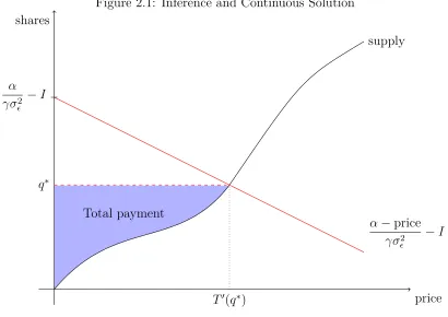
For illustration purposes, I first consider the case where prices are continuous. A supplier
posts an offer to sell at a price and an informed active trader’s buy order walks the book,
picking off these shares. Following rational expectations, the seller must exhibit no regret
in selling shares to the profile of traders that bought them. In Figure 2.1, a supply schedule
generates a purchase choice of q∗ shares. The optimal choice by the active trader is the intersection of supply and incentives to buy shares, α−γσprice2
−I. Given that γσ
2
is common
knowledge, the supplier knows the slope of this curve, and can back out the intercept,
revealing the profile of active traders (α, I). The liquidity supplier considers the profile of
traders who would buy at a given price and quantity and responds with the optimal number
of shares.12
Figure 2.1: Inference and Continuous Solution
Total payment
price shares
supply
q∗
T0(q∗)
α γσ2
−I
α−price
γσ2
−I
To put it more formally, liquidity suppliers compete in transfer schedulesT(·) :R+→ R+
giving the payment for any quantity, q, demanded by an active trader. As a result, the active trader choosesq maximizing E[−e−γW], from (2.6). This is equivalent to maximizing
E[W|α, I] + γ2V[W|α, I]. Variance of holdings is (q+I)2σ2
. From transfer schedules this is
equal to, (q+I)α−T(q)−γ2(q+I)2σ2
. This yields an interior solution for supply schedules
where q∗ = α−γσT0(2q∗)
−I. Here the supply curve in Figure 2.1 is T
0(q), and T0(q∗) is simply
the price at which the last portion of q∗ is supplied.
In typical data, supply schedules are not continuous functions of price, but rather
step functions. This introduces complications to the model, as I show here.13 Solving
12This reasoning is similar to strategies conditional on winning the prize in auctions (see Milgrom and
Weber (1982)), and vote pivotality in juries (see Feddersen and Pesendorfer (1998)). The liquidity supplier must offer enough shares to take advantage of the hedging needs of traders reaching that far in the book while balancing information asymmetry faced at that point as well.
for equilibrium q, the best response quantity demanded by an active trader when utility is u(q|α, I) ≡ −e−γW, is again equivalent to the active trader choosing a q maximizing
E[W|α, I] + γ2V[W|α, I]. Wealth is given by equation 2.7, and the trader maximizes,
(q+I)α | {z }
expected value of shares
−
M
X
r=0
max{0,min{q, Sr} −Sr−1}pr
| {z }
payment to suppliers
− γ
2(q+I)
2σ2
| {z }
volatility penalty
. (2.8)
In equation 2.8, v in wealth as in equation 2.7 is replaced by α, because σ is expectation
0. However, σ shows up in the risk aversion variance of wealth penalty. Because of the
discrete nature of these supply curves, either the active trader reaches a first order condition,
at some point between Sr and Sr+1 for some r, or not, at Sr+1 for some r. In the first
case, α− pm − γ2σ2(2q + 2I) = 0, where pr is s.t. Sr < q < Sr+1. In the second, the
first order condition is not reached, and q = Sr+1 s.t. α −pr − γ2σ2(2q + 2I) > 0 and
α−pr+1 −γ2σ2(2q+ 2I)<0, hence the active trader has exhausted all gains from trade at
price pr, but would lose money trading at pr+1 for the next available liquidity in the book.
The two cases are as follows,
Case 1: interior solution, wherepr is s.t. Sr−1 < q < Sr
q = α−pr
γσ2
−I (2.9)
As can be seen, given a supply schedule and an active trader places an order, liquidity
suppliers can infer a statistic, α
γσ2
−I, for α and I which contains all the information the
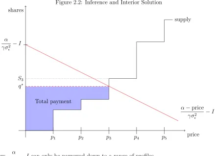
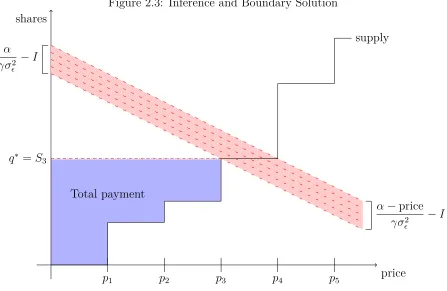
liquidity suppliers can infer about α and I. Case 2: boundary solution, q =Sr
α−pr+1
γσ2
−I < q < α−pr γσ2
−I (2.10)
However, if q∗ =Sr for some r, then inference is not as clear for the liquidity suppliers.
Figure 2.2: Inference and Interior Solution
Total payment
price shares
p1 p2 p3 p4 p5
S3
supply
α γσ2
−I
α−price
γσ2
−I q∗
Now, α
γσ2
−I can only be narrowed down to a range of profiles.
2.3.4
Liquidity Suppliers and the Optimal Supply Problem
I assume that offers at a given price are executed proportionally.14 This means that at price
pr, the bid walks through the orders at a rate s
i r
si r+s−ri
for each supplieriuntil the order moves up the book to the next price. With these solutions I compute the utility of offering shares
for the liquidity supplier at each price pr, which is expected profitability given liquidity
suppliers are risk-neutral. Either q > Sr−1+sir+s
−i
r orSr−1 < q ≤Sr−1+sir+s
−i r .
uL(pr, Sr−1, sir, s
−i r ) =
Eα,,I
" sir1{S
r−1+sir+s
−i
r ≤q}(pr−v) +
sir si
r+s−ri
(q−Sr−1)1{Sr−1<q<Sr−1+sir+s
−i
r }(pr−v) #
(2.11)
14Because the model used here is not explicitly dynamic, assuming that some orders are executed after
Figure 2.3: Inference and Boundary Solution
Total payment
price shares
p1 p2 p3 p4 p5
supply
q∗ =S3
α γσ2
−I
α−price
γσ2
−I
The expected profit is added to the continuation payoff for subsequent prices. For each
number of shares offered, there is an expected profit for that price, and an expected payoff
for subsequent supply. I consider a symmetric equilibrium for liquidity suppliers when the
derivative of this expected profit with the derivative of continuation is 0.15 I leave further
derivation to the appendix, 4.2.
2.4
Estimation
Here I describe my econometric method in which I use a nested fixed point algorithm, as
in Rust (1987)16. Starting with parameter values of the structural model, I find equilibrium
supply curves. Using a pseudo-model17 (following the terminology in Gouri´eroux, Monfort,
15While Back and Baruch (2012) show equilibrium theoretically for only a range of parameter values, I
verify the equilibrium numerically.
16See Rust (1994) and Rust (1996) for further discussion.
17The pseudo-model is referred to as anapproximated model, aninstrumental model, and astatistical model
and Renault (1993)), I fit the generated supply curves to those found in the data. Choosing
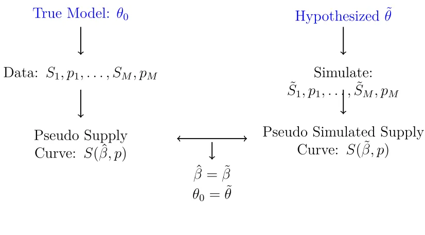
new parameter values, I iterate until I achieve a best fit. This is illustrated in Figure 2.4,
below. In addition, the following sections describe the individual components of this analysis.
Figure 2.4: Indirect Inference
True Model:
θ
0Data:
S
1, p
1, . . . , S
M, p
MPseudo Supply
Curve:
S
( ˆ
β, p
)
Hypothesized ˜
θ
Simulate:
˜
S
1, p
1, . . . ,
S
˜
M, p
MPseudo Simulated Supply
Curve:
S
( ˜
β, p
)
ˆ
β
= ˜
β
θ
0= ˜
θ
2.4.1
Solving for Equilibrium
Players compete in supply schedules at each price successively, as liquidity at lower prices
affects the profitability of liquidity supplied later. In the optimal Markov strategy, liquidity
suppliers’ offers of shares at a given price are based soley on the amount of liquidity offered
up to that point.18 Suppliers consider a trade executing against their supply schedule. The
market order picks off shares at prices at which liquidity is offered, until the order is met. A
liquidity supplier infers what profile of information and liquidity incentives were faced given
the trade reached that deep in the book, and decides how many shares to offer at that price.
Suppliers determine their strategies starting at the limit of economically meaningful share
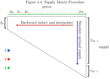
depth and backward induct to find their optimal supply curves.
For interested readers, solving for equilibrium is described in detail in the appendix, 4.4.
18Given the nature of modeling competition in supply, if an optimal strategy exists for this problem, then
2.4.2
Indirect Inference
For estimating model parameters, I use the simulated method of Indirect Inference, following
seminal work in Gouri´eroux, Monfort, and Renault (1993), and Smith (1993).19 I estimate a pseudo-model for data and limit order supply curves simulated from the model. Realizing a
best fit of the model means generating estimates as close together as possible. I find the set
of parameters such that the pseudo-model’s two sets of estimations coincide.20 Coefficients
of the pseudo-model consist of a least squares regression of share quantities on four linear
and nonlinear functions of price.
Let ˆβ denote parameters of the pseudo-model estimated from actual data. Analogously, let ˜βλ(θ) denote parameters estimated from data simulated from the limit order book under parametersθ (λ superscripts the specific simulation). The Indirect Inference estimator ˆθΛ 21
optimizes the following criterion,
ˆ
θΛ ≡arg min
θ∈Θ
βˆ− 1 Λ
Λ
X
λ=1
˜
βλ(θ)
0
Ω
βˆ− 1 Λ
Λ
X
λ=1
˜
βλ(θ)
(2.12)
I explain details of the Indirect Inference method, demonstrate asymptotic normality of
the estimator, and also prove the following proposition in the appendix, 4.5,
Proposition 3. Under assumptions 1–6, ˆθΛ is a consistent estimator of θ0.
19See Goettler and Gordon (2011) for another recent use of Indirect Inference for estimating equilibrium
of a structural model.
20For all estimates, I try different starting values for the parameter search algorithm. In most cases,
the outcomes for the model parameters are the same. When different starting values produced different parameter estimates, I chose the model parameters that led to the lowest criterion function values.
21Λ signifies the number of simulated supply curves analyzed by the pseudo-model. In this paper, I use
2.5
Empirical Results: A Snapshot of Google, October
14-16, 2009
In this section I estimate the model. I examine the limit order book for Google stock (trading
on NASDAQ), using nine episodes bracketing the 2009 third quarter earnings announcement
by Google. Each episode includes a series of observations of the limit order book,
characteriz-ing equilibrium in the limit order market at the time of the episode. Each set of observations
are grouped together to form estimates of the model. I obtain a picture of how information
asymmetry evolved before and after the announcement.
2.5.1
Earnings Announcements, Asymmetric Information
Earnings announcements convey meaningful information about a company. Markets price an
asset consistently with market expectations, but the true profits and losses a company realizes
over the quarter may shift these expectations, causing jumps in asset prices. Trading on this
information could be very profitable and insiders trading on information could undermine
the market. Leading up to an earnings announcement, a Google employee, for example an
upper level manager, who may be a significant Google shareholder, could have information
about the announcement not yet known to the market. Uninformed institutional traders
offer liquidity to this Google employee, keeping in mind that the employee may be trading
based on liquidity preferences, e.g., reducing exposure to the asset, or inside information. If
institutional traders anticipate heavy information trading, depth of the book will be shallow.
However, if they anticipate liquidity trading, supply schedules will become steeper and more
depth will fill the book.
There is an important literature studying returns and markets surrounding earnings
announcements. Linnainmaa (2010) shows that using limit orders changes the inferences one
can make about trading intentions. Examining several regularly identified investor trading
and that much of the inferences about investors’ trading abilities are due to limit orders’
exposure to adverse selection risk. Christophe, Ferri, and Angel (2004) use NASDAQ data
to examine short-selling prior to earnings announcements, and find a significant link between
abnormal short-sales and post-announcement stock returns.22 Similarly, Kaniel, Liu, Saar,
and Titman (2012) consider large individual investor buys and sells on the New York Stock
Exchange, and show corresponding abnormal returns following earnings announcements.23 While these studies analyze price movements and trading volumes, as indirect evidence of
information leakage, I use my structural model to directly quantify changes in information
asymmetry surrounding an earnings announcement. As I show below, the implications of my
results differ from implications one might draw from analyzing price movements and trading
volume.
On Thursday, October 15, 2009, Google closed on NASDAQ at $530, well below the
Wednesday close of $535.50. That afternoon, then CEO Eric Schmidt made the 3rd quarter
earnings announcement, remarking,
Google had a strong quarter–I saw 7% year-over-year revenue growth despite the
tough economic conditions. While there is a lot of uncertainty about the pace of
economic recovery, I believe the worst of the recession is behind us and now feel
confident about investing heavily in the future.24
This was apparently a positive shock to the market; the stock reopened at $546.50 on Friday,
Oct. 16, eventually closing at $550, while market returns were flat these days. Next, I
22Ball and Brown (1968) were the first to note the link between abnormal returns and unexpected earnings
announcements. Foster, Olsen, and Shevlin (1984) replicated these findings regarding abnormal returns, uncovering similar market inefficiencies. Bernard and Thomas (1989) and Bernard and Thomas (1990) show support of the hypothesis of price response delay, rejecting that capital asset pricing systematically underestimates (overestimates) risk surrounding good (bad) news.
23Lee (1992) were early to find patterns regarding strategies of large and small investors. Bartov,
Rad-hakrishnan, and Krinsky (2000), and Bhattacharya (2001) find that investor sophistication is negatively cor-related with abnormal returns–investors with less sophistication underestimate the implications of a surprise earnings announcement. Battalio and Mendenhall (2005) show that investors making large trades respond to earnings forecast errors, while investors making small trades respond to a less-sophisticated signal. See Hirshleifer, Myers, Myers, and Teoh (2008) for contrasting analysis.
examine this through the lens of the structural estimates from my equilibrium limit order
model.
2.5.2
Estimation Results
I estimate the model on three days surrounding the announcement. The earnings
announce-ment was made 4:30 p.m. EST, Oct. 15, a half-hour after the market closed, and estimates
are taken from Oct. 14, 15, and 16, early, midday, and late during trading hours. I
charac-terize information asymmetries and liquidity motivations for trading at each point in time.
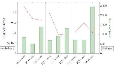
Before turning to my structural estimates, I consider typical measures of information
asymmetry; specifically, I look at the bid-ask spread and the amount of shares offered in the
order book. Figure 2.5 shows an overall downward trend in bid-ask spreads in this three
day period, with a spike in spread in the middle of the day following the announcement,
consistent with Lee, Mucklow, and Ready (1993).25 This hints at an overall reduction in
information asymmetry during this period. Similarly, Figure 2.5 demonstrates the amount
of shares in the first five ticks of the market are low early in the day, high late.
Next I turn to my structural estimates. Results and definitions of terms can be found in
Table 2.2. The level of µI changes a great deal over this period of time, being lower (and
negative, so greater in absolute magnitude, and more hedging preferences for trade) later
in the day than earlier, with a peak (and therefore less liquidity preferences for trade) in
the middle of the day. However, σα changes rapidly, and beginning Oct.14, σ is gradually
increasing. As σα falls and σ rises, the ratio of σα to σ decreases, hence, asymmetric
information drops significantly. Information asymmetry drops from Oct. 14 to Oct. 15,
continuing to fall later on Oct. 15–as evidenced by the increased hedging incentive revealed
in the market at that time in the day. I see this asymmetry fall again on Oct. 16, with a
lower point in the middle of the trading day.
25Lee, Mucklow, and Ready (1993) show that liquidity providers are sensitive to changes in information
Table 2.2: Earnings Announcements Results
This table shows fitted parameters of the true model for the sell side of the Google limit order book surrounding its 3rd quarter earnings announcement, made 4:30 p.m. EST, October 15, 2009. Parameters are estimated from the first five ticks of the book in a set of three samples, one on each side of a time of day, where samples are separated by 15 minutes. The dates and times chosen are early, midday and late on October 14, 15, and 16. Market open at 9 a.m., each early estimate is taken at 10:00 a.m., EST, unless otherwise specified, midday, 1:00 p.m., and late,
3:30 p.m., market closing at 4 p.m. σα is the standard deviation of the informed trader’s signal
about the asset’s true value, and σ is the standard deviation of the white noise around the
informed trader’s signal, both in $. µI andσI are the mean and variance of the inventory of the
informed trader, in shares of Google stock. σS0 is the standard deviation of a calibration variable
representing hidden orders and impatient sellers, in shares of Google. Bootstrap standard errors in parentheses.
Date-Time σα σa µI σI σS0
10/14 early 0.7260 0.0415 -700.106 199.806 20.927
(0.0076) (0.0005) (2.9226) (6.8451) (3.2822)
10/14 mid 0.3367 0.0306 -401.749 111.887 20.005
(0.0066) (0.0020) (5.247) (3.454) (0.2524)
10/14 late 0.5720 0.0216 -1598.362 561.992 19.407
(0.0013) (0.00004) (2.352) (2.667) (0.2983)
10/15 early 0.4375 0.0254 -947.812 148.192 12.030
(0.0009) (0.00009) (0.5244) (3.454) (0.0154)
10/15 mid 0.4274 0.0339 -736.098 230.567 19.861
(0.0026) (0.0001) (2.963) (3.452) (0.1252)
10/15 late 0.4571 0.0284 -2169.115 275.685 20.300
(0.0058) (0.0002) (34.372) (13.408) (1.1364)
10/16 earlyb 0.6871 0.0481 -912.498 81.159 8.0851
(0.0006) (0.00003) (0.1377) (0.3464) (0.0077)
10/16 mid 0.3855 0.0445 -704.534 253.961 20.851
(0.0177) (0.0011) (9.602) (17.688) (0.3929)
10/16 late 0.2933 0.0204 -2376.286 725.681 20.496
(0) (0) (0) (0) (0)
Nc 51 – – – –
Sd 200 – – – –
aThe coefficient of risk aversion, γ never stands alone, meaning that it is estimated directly with σ . I
assumeγ= 1 and show estimates forσ. bThis time was offset by a total of two (2) fifteen minute periods
to 10:30 a.m.. The bid-ask spread was too wide to produce meaningful estimates, and I waited until a point in the day that the market was back in equilibrium. cFor each set of estimates I take 3 samples. Each
sample has a number of instances of the order book. This is the sample size. dI use simulations to fit data.
Figure 2.5: Bid-Ask Spread and Depth
0 5·10−2
0.1 0.15 0.2
Bid-Ask
Spread
shares
10/14–early 10/14–mid 10/14–late10/15–early 10/15–mid 10/15–late10/16-early 10/16–mid 10/16–late
bid-ask
0 500 1,000 1,500 2,000 2,500
Shares
of
Sto
ck
2.5.3
Informedness Ratio
To summarize the implications of parameter estimates on the extent of information
asym-metry and adverse selection, I introduce the informedness ratio. The informedness ratio is
defined as the ratio of the standard deviations of the asset value from the liquidity suppliers’
perspective and the active trader’s perspective. The active trader receives a signal about the
asset’s true value and the liquidity suppliers do not. Therefore, the ratio is simply the ratio
of the standard deviation of the true value from its expectation, and the standard deviation
of the white noise the active trader faces in the signal, which is a natural measure of how
much less informed the liquidity suppliers are compared to the active trader. The true value
informedness ratio is defined as,
σv
σ
= q
σ2
α+σ2
σ
≡Informedness Ratio26 (2.13)
The informedness ratio has no absolute cardinal meaning. However, a higher value may
be indicative of large asymmetry in information or a preponderance of information trading,
while a lower value indicates more liquidity-motivated trading and hence, less information
asymmetry.
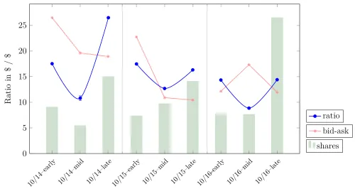
The informedness ratio from my results is plotted in Figure 2.6. There is a pronounced
downward trend in the informedness ratio over the three day period, implying a reduction in
information asymmetry. The informedness ratio is rather high late on Oct. 14. It falls steeply
by Oct. 15, settling around 17 that day. This shows that the market responded to asymmetry
that is reduced the day of the earnings announcement. Whatever information traders were
ready to trade on, prior to the earnings announcement, the market is no longer responding to
it once the earnings announcement is made. However, this information asymmetry dissipates
further, as evidenced by continued decline in the informedness ratio the day after the earnings
announcement is made. It reaches 14 and then 8 after being double that the day before.
This plot indicates that the market behaves as if active traders were better informed
(relative to uninformed liquidity suppliers) the day before the announcement, and that this
informedness dissipated by the day of the announcement. The fall in the informedness ratio
between Oct. 14 late and Oct. 15 early contrasts with the trend in the bid-ask spread,
which peaked during Oct. 15 early, as shown in Figure 2.5. Overall, the downward trend
in the informedness ratio corroborates a similar trend in the bid-ask spread, however, the
informedness ratio implies that the decline in information asymmetry began earlier.
26The coefficient of risk aversion, γ never stands alone, meaning that it is estimated directly with σ
. I
Figure 2.6: Informedness Ratio
shares bid-ask
10/14–early 10/14–mid 10/14–late 10/15–early 10/15–mid 10/15–late 10/16-early 10/16–mid 10/16–late
0 5 10 15 20 25
Ratio
in
$
/
$
ratio
2.6
Robustness Checks: Levels of Competition
In limit order data, individual-level order placement goes unobserved. However, the model
specifies a number of traders. I estimate the model using n = 5, a choice resulting from a specification search over different values ofn.
2.6.1
Comparison of Fit
I show that the market behaves as if there are more liquidity suppliers than two and fewer
than ten. If the model were to fit well with n = 5 liquidity suppliers, and not as well with
n = 2 or n = 10, this would be evidence the market behaves as if there are effectively five liquidity suppliers competing for the business of active traders. Model fit and estimates for
Table 2.3: Robustness Checks
This table shows comparative fitted parameters of the true model for market structures with two, five, and ten liquidity suppliers for the sell side of the Google limit order book surrounding its 3rd quarter earnings announcement, made 4:30 p.m. EST, October 15, 2009. The market for Google opens at 9 a.m., EST, and unless otherwise noted, early refers 10:00 a.m., mid refers to 1:00 p.m., and late refers to estimates being made for data at 3:30 p.m., market closing at 4:00
p.m. σα is the standard deviation of the informed trader’s signal about the asset’s true value,
andσ is the standard deviation of the white noise around the informed trader’s signal, both in
$. µI and σI are the mean and variance of the inventory of the informed trader, in shares of
Google stock, where greater magnitude means more liquidity preferences. σS0 is the standard
deviation of a calibration variable representing hidden orders and impatient sellers, in shares of Google. Fit shows the mean-squared error of the estimates, and a lower number is a better fit. The model fits better with number of liquidity suppliers being five rather than two, hence markets behave as if they have five dealers, as opposed to two. This is evidence that modern limit order markets are more efficient than hypothetical dealer markets–characterized by one, or maybe two dealers–would be. Standard errors in parentheses.
σα σ µI σI σS0
n fit
10/14 late 2 52,244.2 0.4253 0.0391 -2633.938 814.957 20.607
5 7651.4 0.5720 0.0216 -1598.362 561.992 19.407
10 10,863.5 0.2794 0.0227 -527.943 176.344 17.314
10/15 early 2 214.0 0.3754 0.0579 -1454.298 415.548 20.388
5 6.0 0.4375 0.0254 -947.812 148.192 12.030
10 55.4 0.6434 0.0698 -285.119 190.829 22.548
10/15 mid 2 6296.4.8 0.3608 0.0436 -1853.380 542.495 20.210
5 90.0 0.4274 0.0339 -736.098 230.567 19.861
10 367.5 0.3772 0.0327 -366.799 105.985 20.116
10/15 late 2 95,737.8 0.2632 0.0209 -2193.646 265.143 20.225
5 83.9 0.4571 0.0284 -2169.115 275.685 20.300
10 297.5 0.1925 0.0433 -692.216 294.226 20.538
10/16 earlya 2 9631.1 0.4286 0.0424 -2361.003 683.236 20.436
5 687.7 0.6871 0.0481 -912.431 80.932 8.004
10 581.4 0.2484 0.0214 -463.436 137.343 19.778
aThis time was offset by a total of two (2) fifteen minute periods to 10:30 a.m.. The bid-ask spread was too wide
Table 2.3 contains fitted θs for five dates and times examined earlier. I also include θs for n = 2 and n = 10 to contrast specification fits. The model fits are better in four of the five dates and times. Market data is fitted by the model consistently better for n = 5 over
n= 2 with only one instance of a fit worse than n = 10.
2.6.2
Comparing Limit Order Markets and Dealer Markets
The model I estimate fits better with n= 5 than it does with n = 2 or n = 10. Looking at
n= 2, corresponds to estimating a dealer market. I investigate the change in welfare moving from dealer to limit order markets. Historically, NASDAQ, New York Stock Exchange, and
others, depended on dealers or market makers to facilitate the market for an asset. More
recently, modern markets have employed a direct trading scheme in the form of a limit order
market. In dealer markets, traders never directly interact. Instead, a trader would make
known to a dealer that she was interested in selling shares of a stock. The dealer would post
terms for trade, and the trader would sell as much as she wished according to those terms.
The dealer would then sell those shares on the other side of the market. This way a trader
could always trade and never had to wait for terms to be met as long as the dealer was there
to take the other side of any transaction. Limit order markets are centralized, but trade
need not go through a single intermediary.
While the move from dealer markets to limit order markets is pervasive, it is not clear
they are better in terms of welfare. It may be the case that while limit order markets bypass
the middleman, that liquidity is more available under a dealer market scheme. However, it
may be that the ability of any trader to play the role of dealer allows for greater liquidity
provision.
The difficulty of characterizing the limit order book theoretically makes this welfare
question very difficult to analyze. Pagnotta (2010) presents a computational model that
nests dealer and limit order markets, allowing for a comparison of utilities. Finding that
does better than its historical counterpart.
The model estimated here also nests dealer and limit order markets, and is amenable
to a welfare comparison of the two. Because active traders and liquidity suppliers trade
with each other, the model is essentially a dealer market. If liquidity suppliers offer a large
number of shares early, then the informed traders they face at higher prices in the book
will likely have a strong signal about the price of the asset, decreasing expected profits.
In a monopolistic setting, a liquidity supplier bears the entirety of this loss, and so will
offer liquidity at higher prices, leading to a large bid-ask spread. However, adding liquidity
suppliers increases incentives to offer liquidity at low prices. With a large number of suppliers,
there is close to efficient liquidity provision and a small bid-ask spread. I showed earlier that
the model fit is better for n = 5 than it is for n = 2. I demonstrate here that increasing the number of liquidity suppliers in the market raises welfare. Because a large number of
dealers is unambiguously good, and the model fits better forn = 5, data confirms Pagnotta’s results; limit order markets are better for welfare than dealer markets.
2.6.3
Counterfactual Utilities
I calculate profitability for liquidity suppliers and certainty-equivalent utility for the active
trader. These values will be useful in considering counterfactual utilities, comparing social
welfare in dealer and limit order markets. Interested readers can find relevant calculations
in the appendix, 4.3.
I generate counterfactual markets, varying the number of liquidity suppliersn = 1, . . . ,50, ranging from a monopoly to relative competition. Using these simulated markets, I compute
expected profits to liquidity suppliers and the certainty-equivalent utility increase for active
traders. Table 2.4 presents counterfactual estimates for five dates and times examined in the
earnings announcements section. For each example, profits to liquidity suppliers go down
as the number of competitors increases. Conversely, certainty-equivalent utility goes up for