Inference for stochastic volatility model using time change transformations

Munich Personal RePEc Archive

Inference for stochastic volatility model

using time change transformations

Kalogeropoulos, Konstantinos and Roberts, Gareth O. and

Dellaportas, Petros

University of Cambridge, Engineering Department - Signal

Processing Lab, University of Warwick, Statistics Department,

Athens University of Economics and Business, Statistics Department

2007

Online at

https://mpra.ub.uni-muenchen.de/5697/

Inference for stochastic volatility models using time

change transformations

Konstantinos Kalogeropoulos

University of Cambridge, Department of Engineering - Signal Processing Lab

Gareth O. Roberts

University of Warwick, Department of Statistics

Petros Dellaportas

Athens University of Economics and Business, Department of Statistics

October 14, 2007

Abstract

We address the problem of parameter estimation for diffusion driven stochastic

volatil-ity models through Markov chain Monte Carlo (MCMC). To avoid degeneracy issues we

introduce an innovative reparametrisation defined through transformations that operate

on the time scale of the diffusion. A novel MCMC scheme which overcomes the inherent

difficulties of time change transformations is also presented. The algorithm is fast to

implement and applies to models with stochastic volatility. The methodology is tested

through simulation based experiments and illustrated on data consisting of US treasury

bill rates.

Keywords: Imputation, Markov chain Monte Carlo, Stochastic volatility

1

Introduction

Diffusion processes provide natural models for continuous time phenomena. They are used

extensively in diverse areas such as finance, biology and physics. A diffusion process is defined

through a stochastic differential equation (SDE)

where W is standard Brownian motion. The drift µ(.) and volatility σ(.) reflect the

instan-taneous mean and standard deviation respectively. In this paper we assume the existence

of a unique weak solution to (1), which translates into some regularity conditions (locally

Lipschitz with a linear growth bound) onµ(.) andσ(.); see chapter 5 of Rogers and Williams

(1994) for more details.

The task of inference for diffusion processes is particularly challenging and has received

remarkable attention in the recent literature; see Sørensen (2004) for an extensive review. The

main difficulty is inherent in the nature of diffusions which are infinite dimensional objects.

However, only a finite number of points may be observed and the marginal likelihood of these

observations is generally unavailable in closed form. This has stimulated the development

of various non-likelihood approaches which use indirect inference (Gouri´eroux et al., 1993),

estimating functions (Bibby and Sorensen, 1995), or the efficient method of moments (Gallant

and Tauchen, 1996); see also Gallant and Long (1997).

Most likelihood based methods approach the likelihood function through the transition

density of (1). Denote the observations by Yk,k= 0, . . . , n, and with tk their corresponding

times. If the dimension of Yk equals that of X (for each k) we can use the Markov property

to write the likelihood, given the initial pointY0, as:

L(Y, θ|Y0) =

n

Y

k=1

pk(Yk|Yk−1;θ,∆), ∆ =tk−tk−1 (2)

The transition densitiespk(.) are not available in closed form but several approximations are

available. They may be analytical, see A¨ıt-Sahalia (2002), A¨ıt-Sahalia (2005), or simulation

based, see Pedersen (1995), Durham and Gallant (2002). They usually approximate the

likelihood in a way so that the discretisation error can become arbitrarily small, although

the methodology developed in Beskos et al. (2006) succeeds exact inference in the sense that

it allows only for Monte Carlo error. A potential downside of these methods may be their

dependence on the Markov property. In many interesting multidimensional diffusion models

the observation regime is different and some of their components are not observed at all.

A famous such example is provided by stochastic volatility models, used extensively to

model financial time series such as equity prices (Heston, 1993; Hull and White, 1987; Stein

and Stein, 1991), or interest rates (Andersen and Lund, 1998; Durham, 2002; Gallant and

Tauchen, 1998). A stochastic volatility model is usually represented by a 2-dimensional

  dXt dαt  =  

µx(Xt, αt, θ)

µα(αt, θ)

 dt+

 

σx(αt, θ) 0

0 σα(αt, θ)

    dBt dWt 

, (3)

where X denotes the observed equity (stock) log-price or the short term interest rate with

volatilityσx(.), which is a function of a latent diffusionα. For the diffusion in (3), the Markov

property may no longer hold; the distribution of a future stock price depends (besides the

current price) on the current volatility which in turn depends on the entire price history.

Stochastic volatility models are used

An alternative approach to the problem adopts Bayesian inference utilizing Markov chain

Monte Carlo (MCMC) methods. Adhering to the Bayesian framework, a prior p(θ) is first

assigned on the parameter vector θ. Then, given the observations Y, the posterior p(θ_|Y)

can be explored through data augmentation (Tanner and Wong, 1987), treating the

unob-served paths of X (paths between observations) as missing data. The resulting algorithm

alternates between updatingθandX. Initial MCMC schemes following this programme were

introduced by Jones (1999); see also Jones (2003), Eraker (2001) and Elerian et al. (2001).

However, as noted in the simulation based experiment of Elerian et al. (2001) and established

theoretically by Roberts and Stramer (2001), any such algorithm’s convergence properties

will degenerate as the number of imputed points increases. The problem may be overcome

with the reparametrisation of Roberts and Stramer (2001), and this scheme may be applied

in all one-dimensional and some multi-dimensional contexts. However this framework does

not cover general multidimensional diffusion models. Chib et al. (2005) and Kalogeropoulos

(2007) offer appropriate reparametrisations but only for a class of stochastic volatility

mod-els. Alternative reparametrisations were introduced in Golightly and Wilkinson (2007); see

also Golightly and Wilkinson (2006) for a sequential approach.

In this paper we introduce a novel reparametrisation that, unlike previous MCMC

ap-proaches, operates on the time scale of the observed diffusion rather than its path. This

facilitates the construction of irreducible and efficient MCMC schemes, designed

appropri-ately to accommodate the time change of the diffusion path. Our approach is general enough

to cover almost every stochastic volatility model used in practice. The paper is organized as

follows: Section 2 elaborates on the need for a transformation of the diffusion to avoid

prob-lematic MCMC algorithms. In Section 3 we introduce time change transformations whereas

Section 4 provides the details for the corresponding non-trivial MCMC implementation. The

in section 5, and on US treasury bill rates in section 6. Finally, section 7 concludes and

provides some relevant discussion.

2

The necessity of reparametrisation

A Bayesian data augmentation scheme bypasses a problematic sampling from the posterior

π(θ|Y) by introducing a latent variableX that simplifies the likelihoodL(Y;X, θ). It usually

involves the following two steps:

1. Simulate _X conditional on Y and θ.

2. Simulate θ from the augmented conditional posterior which is proportional to _L(Y;_X, θ)π(θ).

It is not hard to adapt our problem to this setting. Y represents the observations of the

price processX. The latent variables_X introduced to simplify the likelihood evaluations are

discrete skeletons of diffusion paths between observations or entirely unobserved diffusions.

In other words,_X is a fine partition of multidimensional diffusion with driftµX(t, Xt, θ) and

diffusion matrix

ΣX(t, Xt, θ) = σ(t, Xt, θ) × σ(t, Xt, θ)′,

and the augmented dataset is _Xiδ, i= 0, . . . , T /δ, whereδ specifies the amount of

augmen-tation. The likelihood can be approximated via the Euler scheme

LE(Y;X, θ) =

T /δ

Y

i=1

p(Xiδ|X(i−1)δ), Xiδ|X(i−1)δ∼ N X(i−1)δ+δµX(.), δΣX(.)

,

which is known to converge to the true likelihood L(Y;X, θ) for small δ (Pedersen, 1995).

Another property of diffusion processes relates ΣX(.) to the quadratic variation process.

Specifically we know that

lim

δ→0

T /δ

X

i=1

Xiδ− X(i−1)δ

Xiδ− X(i−1)δ

T

=

Z T

0

ΣX(s,Xs, θ)ds a.s.

The solution of the equation above determines the diffusion matrix parameters. Hence,

there exists perfect correlation between these parameters and _X as δ _→ 0. This has

dis-astrous implications for the mixing and convergence of the MCMC chain as it translates

into reducibility for δ _→ 0. This issue was first noted by Roberts and Stramer (2001) for

Nevertheless, it is not an MCMC specific problem. It turns out that the convergence of its

deterministic analogue, EM algorithm, is problematic when the amount of information in

the augmented data _X strongly exceeds that of the observations. In our case _X contains an

infinite amount of information for δ→0.

The problem may be resolved if we apply a transformation so that the algorithm based

on the transformed diffusion is no longer reducible as δ → 0. Roberts and Stramer (2001)

provide appropriate diffusion transformations for scalar diffusions. In a multivariate context

this requires a transformation to a diffusion with unit volatility matrix; see for instance

Kalogeropoulos et al. (2007). A¨ıt-Sahalia (2005) terms such diffusions as reducible and

proves the non-reducibility of stochastic volatility models that obey (3). The transformations

introduced in this paper follow a slightly different route and target the time scale of the

diffusion. One of the appealing features of such a reparametrisation is the generalisation to

stochastic volatility models.

3

Time change transformations

For ease of illustration we first provide the time change transformation and the relevant

likelihood function for scalar diffusion models with constant volatility. Nevertheless, one

of the main advantages of this technique is the applicability to general stochastic volatility

models.

3.1 Scalar diffusions

Consider a diffusionX defined through the following SDE:

dXt=µ(t, Xt, θ)dt+σdWtX, 0< t <1 σ >0. (4)

Without loss of generality, we assume a pair of observationsX0=y0 andX1 =y1. For more

data, note that the same operations are possible for every pair of successive observations

that are linked together through the Markov property. We introduce the latent ‘missing’

path of X for 0 _≤ t _≤ 1, denoted by Xmis, so that X = (y0, Xmis, y1). In the spirit of

Roberts and Stramer (2001), the goal is to write the likelihood for θ, σ with respect to

a parameter-free dominating measure. Using Girsanov’s theorem we can get the

driftless diffusionM =σdW_tX which represents Wiener measure and is denoted byWX_{. We}

can write

dP(X)

dWX =G(t, X, θ, σ) = exp

Z T

0

µ(s, Xs, θ)

σ2 dXs− 1 2

Z T

0

µ(s, Xs, θ)2

σ2 ds

.

By factorizing WX ₌ WX_{y ×Leb(y1)×f(y1;σ}2_{), where y1 ∼ N(y0, σ}2_{) and Leb(.) denotes}

Lebesgue measure, we obtain

dP_(Xmis_{, y0, y1)}

d

WX

y ×Leb(y)

=G(t, X, θ, σ)f(y1;σ),

where clearly the dominating measure depends on σ, since it reflects a Brownian bridge with

volatilityσ.

Now consider the time change transformation which first introduces a new time scale

η(t, sigma))

η(t, σ) =

Z t

0

σ2ds=σ2t, (5)

and then defines the new transformed diffusion U as

Ut=

  

X_η−1_(t,σ), 0≤t≤σ2,

M_η−1_(t,σ), t > σ2.

The definition for t > σ2 is needed to ensure that tU is well defined for different values of

σ2 _{>0 which is essential in the context of a MCMC algorithm. Using standard time change}

properties, see for example Oksendal (2000), the SDE for U is

dUt=

  

1

σ2µ(t, Ut, θ)dt+dW_tU 0≤t≤σ2,

dW_tU, t > σ2,

whereWU is another Brownian motion at the time scale ofU. By using Girsanov’s theorem

again, the law of U, denoted by P_{, is given through its Radon-Nikodym derivative with}

respect to the law WU _{of the Brownian motionW}U _{at theU−time scale:}

dP

dWU = G(t, U, θ, σ) = exp

Z +∞

0

µ(s, Us, θ)

σ2 dUs− 1 2

Z +∞

0

µ(s, Us, θ)2

σ4 ds

= exp

( Z σ2

0

µ(s, Us, θ)

σ2 dUs− 1 2

Z σ2

0

µ(s, Us, θ)2

σ4 ds

)

If we condition the Wiener measure ony at the new time scale, the likelihood can be written

with respect to a Brownian bridge measure WU_{y as}

dP_{(U, y0, y1) =G(t, U, θ, σ)f(y1;σ)d}WU_{y ×Leb(y) .}

However, this Brownian bridge is conditioned on the event U_σ2 =y₁ and therefore contains

the parameterσ. For this reason we introduce a second transformation which applies to both

the diffusion’s time scale and its path. Define

U_t0 = (σ2₋t)Z_t/{σ2_(σ2_−t)}, 0≤t < σ2, (7)

U_t0 =Ut−(1−

t σ2)y0−

t

σ2y1, 0≤t < σ 2_.

Note that this transformation is 1-1. Its inverse is given by

Zt=

1 +σ2_t

σ2 U 0

σ4_t/(1+σ2_t), 0≤t <+∞.

Applying Ito’s formula and using time change properties we can also obtain the SDE of Z

based on another driving Brownian motion WZ operating at the Z−time:

dZt=

µt,₁₊σ_tσ22ν(Zt, σ), θ

+ν(Zt)σ2

1 +tσ2 dt+dW

Z

t , 0≤t <+∞, (8)

whereν(Zt, σ) =Ut. This operation essentially transforms to a diffusion that runs from 0 to

+∞ preserving the unit volatility. We can re-attempt to write the likelihood using Girsanov

theorem and condition the dominating measure on y1 to obtain WZy,

dP_{(Z, y0, y1)}

d

WZ

y ×Leb(y)

=G(t, Z, θ, σ)f(y1;σ). (9)

Despite the fact thatG(Z, θ, σ) contains integrals defined in (0, +∞), it is always finite

being an 1₋1 transformation of the Radon-Nikodym derivative betweenP_{(U) and}WU _given

by (6). Using the following lemma, we prove that WZ_{y is the law of the standard Brownian}

motion and hence the likelihood is written with respect to a dominating measure that does

not depend on any parameters.

Lemma 3.1 Let W be a standard Brownian motion in[0, +_∞). Consider the process defined

for 0_≤t_≤T

Bt= (T −t)Wt/{T(T−t)}+ (1−

t T)y0+

t

Then B is a Brownian bridge from y0 at time 0 to y1 at time T.

Proof: See (Rogers and Williams, 1994, IV.40.1) for the casey0 = 0,T = 1. The extension

for general y0 and T is trivial.

Corollary 3.1 The measure WZ_{y is standard Wiener measure.}

Proof: Note that WU_{y reflects a Brownian bridge from y0 at time 0 to y1 at time T and}

we obtained WZ

y by using the transformation of Lemma 3.1. Since this transformation is

1−1, U is a Brownian bridge (under the dominating measure) if and only if Z is standard

Brownian motion.

Note that WZ_{y is the probability law of the driftless version of the conditional diffusion Z,}

whereas the SDE in (8) corresponds to the unconditional version of Z itself. The conditional

SDE ofZ is generally not available but this does not create a problem. For the path updates

we may use the fact that

dP

dWZ y

(Z_|y0, y1) =G(t, Z, θ, σ)

f(y1;σ)

fP_(y

1;σ) ∝

G(t, Z, θ, σ), (10)

where P_{y is the law of the conditional version of Z and f}P_{(.) is the density of y1 under} P_.

Both P_{y and f}P_{(.) are generally unknown but G(.) and f(.), which appear in (9) and (10),}

are available.

3.2 Stochastic volatility models

Consider the general class of stochastic volatility models with SDE given by (3). Without

loss of generality, we may assume a pair of observations (X0 = y0, X1 = y1) due to the

Markov property of the 2-dimensional diffusion (X, α). The likelihood can then be divided

into two parts: The first contains the marginal likelihood of the diffusionαand the remaining

part corresponds to the diffusion X conditioned on the path ofα

P_{θ(X, α) =}P_θ(α)P_θ(X|α).

Denote the marginal likelihood forαby_Lα(α, θ). To overcome reducibility issues arising from

the paths of α one may use the reparametrisations of Chib et al. (2005) or Kalogeropoulos

(2007). The relevant transformations of the latter are

βt=h(αt, θ),

∂h(αt, θ)

∂αt

γt=βt−β0, βt=η(γt),

and the marginal likelihood for the transformed latent diffusion γ becomes

Lγ(γ, θ) =

dP

dP(γ) =G{η(γ), θ}. (11)

By letting αt=gtγ=h−1(η(γt), θ), the SDE of X conditional on γ becomes:

dXt=µx(Xt, gtγ, θ)dt+σx(gtγ, θ)dBt, 0≤t≤1.

Given the paths of the diffusion α, the volatility function σx(gγt, θ) may be viewed as a

deterministic function of time. The situation is similar to that of the previous section. We

can introduce a new time scale

η(t, γ, θ) =

Z t

0

σ_x2(g_tγ, θ)ds,

T =η(tk, γ, θ),

and define U with the new time scale as before (M is a Brownian motion on the U−time

scale)

Ut=

  

X_η−1_(t), 0≤t≤T,

M_η−1_(t), t > T.

(12)

The SDE for U now becomes

dUt=

(

µx Ut, γη−1_(t,γ,θ), θ

σ2

x(γη−1_(t,γ,θ), θ)

)

dt+dW_tU, 0_≤t_≤T.

We obtain the Radon Nikodym derivative between the distribution ofU with respect to that

of the Brownian motion WU,

dP

dWU = G(U, γ, θ),

and introduce WU_{y as before. The density of y1 under} WU_{, denoted byf(y, γ, θ), is just}

f(y1;γ, θ)≡N(y0, T).

The dominating measure WU

y reflects a Brownian motion conditioned to equal y at a

parameter depended time T = η(tk+1, γ, θ). To remove this dependency we introduce a

U_t0= (T ₋t)Z_t/{T(T−t)}, 0_≤t < T, (13)

U_t0=Ut−(1−

t T)y0−

t

Ty1, 0≤t < T.

Therefore, the SDE for Z is now given by

dZt=

T

1 +tT

  

µ₁₊T_tTν(Zt), γk(t,γ,θ), θ

σ2

x(γk(t,γ,θ), θ)

+ν(Zt)

  

dt+dW_tZ, 0_≤t <_∞,

where k(t, γ, θ) denotes the initial time scale of X and ν(Zt) =Ut.

Conditional on γ, the likelihood can be written in a similar manner as in (9):

dP

d

WZ

y ×Leb(y)

(Z_|y0, y1, γ) =G(Z, γ, θ)f(y1;γ, θ) (14)

It is not hard to see thatWZ_{y reflects a standard Wiener measure and therefore the dominating}

measure is independent of parameters. To obtain the full likelihood we need to multiply the

two parts given by (11) and (14).

3.3 Incorporating leverage effect

In the previous section we made the assumption that the increments of X and γ are

inde-pendent, in other words we assumed no leverage effect. This assumption can be relaxed in

the following way: In the presence of a leverage effect ρ, the SDE ofX conditional onγ can

be written as

dXt=µx(Xt, gγt, θ)dt+ρσx(gtγ, θ)dWt+

p

1₋ρ2_σ

x(gγt, θ)dBt, 0≤t≤tk,

where W is the driving Brownian motion of γ). Note that given γ, W can be regarded as

a function of γ and its parameters θ. Therefore, the term ρσx(gγt, θ)dWt can be viewed as

a deterministic function of time, and it can be treated as part of the drift of Xt. However,

this operation introduces additional problems as the assumptions ensuring a weakly unique

solution to the SDE of X are violated. To avoid this issue we introduce the infinitesimal

transformation

Xt=H(Ht, ρ, γ, θ) =Ht+

Z t

0

which leads us to the following SDE for H:

dHt=µx{H(Xt, ρ, γ, θ), gγt, θ}dt+

p

1₋ρ2_σ

x(gγt, θ)dBt, 0≤t≤tk.

We can now proceed as before, definingU andZ based on the SDE ofH in a similar manner

as in (12) and (13) respectively.

3.4 State dependent volatility

Consider the family of state dependent stochastic volatility models where conditional on γ,

the SDE ofX may be written as:

dXt=µx(Xt, gtγ, θ)dt+σ1(gtγ, θ)σ2(Xt, θ)dBt, 0≤t≤tk.

This class contains among others, the models of Andersen and Lund (1998), Gallant and

Tauchen (1998), Durham (2002), Eraker (2001). In order to apply the time change

transfor-mations of section 3.2, we should first transform X to ˙Xt, through ˙Xt=h(Xt, θ), so that it

takes the form of (3). Such a transformation, which may be viewed as the first transformation

in Roberts and Stramer (2001), should satisfy the following differential equation

∂h(Xt, θ)

∂Xt

= 1

σ2(Xt, θ)

.

The time change transformations forU andZ may then be defined on the basis of ¨Xthat

will now have volatility σ1(gγt, θ). The transformation h(.) also applies to the observations

( ˙y0, ˙y1) which are now functions of parameters. This would translated in a parameter

dependent likelihood dominating measure, had it not been for the second step in (12) which

in this case acts like the second transformation in Roberts and Stramer (2001). Note that

the parameters of σ2(Xt, θ) enter the reparametrised likelihood in two ways: first through

thef(y;γ, θ) which now should include the relevant Jacobian term, and second through the

drift of Z which is centered at 0 based on the transformed observations.

3.5 Multivariate stochastic volatility models

We may use the techniques of section 3.3 to define time change transformations for

multidi-mensional diffusions. Consider a d₋dimensional version of the SDE in (4) whereσ now is a

2×2 matrix ([σ]ij =σij). As noted in Kalogeropoulos et al. (2007), the mapping between

parameters. A way to achieve this, is by allowing σ to be the lower triangular matrix that

produces the Cholesky decomposition ofσσT. Ford= 2, the SDE of such a diffusion is given

by

dX_t{1}=µ(X_t{1}, X_t{2}, θ)dt+σ11dBt,

dX_t{2}=µ(X_t{1}, X_t{2}, θ)dt+σ21dBt+σ22dWt.

The time change transformations for X{1} _{will be exactly as in section 3.1. For X}{2}

note that given X{1} the term σ21dBt is now a deterministic function of time and may be

treated as part of the drift. Thus, we may proceed following the route of the section 3.3.

Similar transformations can be applied for diffusions that have, or may be transformed

to have, volatility functions independent of their paths. For example we may assume two

correlated price processes with correlation ρx:

[σ]11=σx{1}(gtγ, θ),

[σ]21=ρxσx{2}(gtγ, θ),

[σ]22=

p

1₋ρ2

xσx{2}(gγt, θ).

We may proceed in a similar manner for multivariate stochastic volatility models of general

dimension d.

4

MCMC implementation

The construction of an appropriate data augmentation algorithm involves several issues. The

time change transformations introduce three interesting features to the MCMC algorithm

which we address separately: the presence of three time scales; the need to update diffusion

paths that run from 0 to +∞; and the fact that time scales depend on parameters. For

ease of illustration we will assume the simple case of a univariate diffusion with constant

volatility and a pair observations (X0=y0 and X1 =y1). Extensions and generalisations of

the algorithm for stochastic volatility models are noted where appropriate.

4.1 Three time scales

We introduce m intermediate points of X at equidistant times between 0 and 1, to give

large enough for accurate likelihood approximations and any error induced by the time

discretisation is negligible for the purposes of our analysis.

Given a value of the time scale parameter σ, we can get theU₋time points by applying

(5) to each one of the existing points X, so that

Uσ2_i/(m+1) =X_i/(m+1), i= 0,1, . . . , m+ 1.

Note that it is only the times that change, the values of the diffusion remain intact. In a

stochastic volatility model we would use the quantities

Z _mi+1

+1

i m+1

σ_x2(.)ds

for each pair of consecutive imputed points.

The points ofZ are multiplied by a time factor which corrects the deviations from unit

volatility. The Z₋time points may be obtained by

tZ_i = σ

2_{i/(m+ 1)}

σ2_(σ2_−σ2_{i/(m+ 1))}, i= 0,1, . . . , m.

Clearly this does not apply to the last point which occurs at time +∞. Therefore, the paths

of X, or U, are more convenient and may be used for likelihood evaluations exploiting the

fact that the relevant transformations are 1-1. However, the component of the relevant Gibbs

sampling scheme is the diffusion Z.

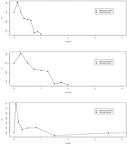
Figure 1 shows a graphical representation of X, U and Z plotted against their

corre-sponding time scales for σ=√2 andm= 7. AlthoughX andU have the same values, their

volatilities are √2 and 1 respectively. The ending point of Z does not appear on the graph

as it occurs at time +_∞.

[Figure 1 about here.]

4.2 Updating the paths of Z

The paths of Z may be updated using an independence sampler with the reference measure

as a proposal. Here WZ _{reflects a Brownian motion at the Z−time which is fixed given}

the current values of the time-scale parameter(s). An appropriate algorithm is given by the

following steps.

• Step 2: Transform back to U∗, using (7).

• Step 3: Accept with probability: minn1,_GG(_(UU∗∗,θ,σ_,θ,σ)₎

o

.

4.3 Updating time scale parameters

The updates of parameters that define the time scale, such as σ, are of particular interest.

In almost all cases, their conditional posterior density is not available in closed form, and

Metropolis steps are inevitable. However, the proposed values of these parameters will imply

different Z− time scales. In other words, for each potential proposed value for σ there

exists a different set of Z₋points needed for accurate approximations of the likelihood the

Metropolis accept-reject probabilities. In theory, this would pose no issues had we been able

to store an infinitely thin partition ofZ, but of course this is not possible.

We use retrospective sampling ideas; see Papaspiliopoulos and Roberts (2005) and Beskos

and Roberts (2005) for applications in different contexts. Under the assumption of a

suf-ficiently fine partition of Z, all the non-recorded intermediate points contribute nothing to

the likelihood and they are irrelevant in that respect; the set of recorded points is sufficient

for likelihood approximation purposes. Alternatively, we may argue that their distribution is

given by the likelihood reference measure which reflects a Brownian motion. Thus, they can

be drawn after the proposal of the candidate value of the time scale parameter. To ensure

compatibility with the recorded partition of Z, it suffices to condition on their neighboring

points. This is easily done using standard Brownian bridge properties: Suppose that we

want to simulate the value of Z at time tb which fall between the recorded values at times

ta and tc, so thatta ≤ tb ≤ tc. Denote by Zta and Ztc the corresponding Z values. Under

the assumption that Z is distributed according toWZ_{y betweenta and tc we have that}

Ztb|Zta, Ztc ∼N

(tb−ta)Ztc+ (tc−tb)Zta

tc−ta

, (tb−ta)(tc−tb) tc−ta

. (15)

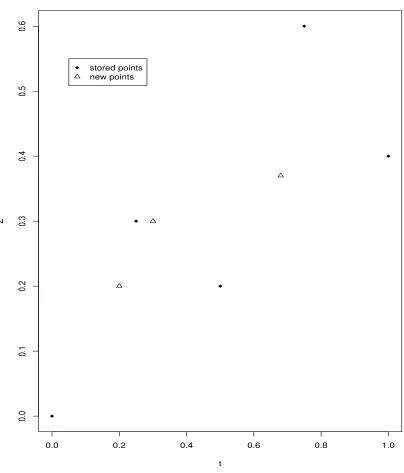
The situation is pictured in Figure 2, where the black bullets represent the stored points and

the triangles the new points required for a proposed value of σ. The latter should be drawn

retrospectively given the former via (15).

[Figure 2 about here.]

A suitable algorithm for the σ₋updates may be summarized through the following steps:

• Step 2: Repeat for each pair of successive points:

– Use (5) and (7) to get the new times associated with it.

– Draw the values of Z at the new times using (15).

– Transform back to U∗, using (7).

Form the entire path U∗ by appropriately joining its bits.

• Step 3: Accept with probability: minn1,G_G(U_(U∗∗,θ,σ_,θ,σ∗)₎f_f(_(yy;_;σ_σ∗₎)

o

.

Note that in a stochastic volatility model the paths of the transformed diffusion γt are

associated with the time scale of the Z. Therefore a similar algorithm may be used for their

updates.

5

Simulations

As discussed in section 2, appropriate reparametrisations are necessary to avoid issues

re-garding the mixing and convergence of the MCMC algorithm. In fact, the chain becomes

reducible as the level of augmentation increases. This is also verified by the numerical

ex-amples performed in Kalogeropoulos (2007) even in very simple stochastic volatility models.

In this section we perform a simulation based experiment to check the immunity of MCMC

schemes to increasing levels of augmentation, as well as the ability of our estimation

proce-dure to retrieve the correct values of the diffusion parameters despite the fact that the series

is partially observed at only a finite number of points. We simulate data from the following

stochastic volatility model

dXt = κx(µx−Xt)dt+ρexp(αt/2)dWt+

p

1₋ρ2_exp(α

t/2)dBt,

dαt = κα(µα−αt)dt+σdWt,

where B and W are independent Brownian motions, andρreflects the correlation between the

increments of X and α, also term as leverage effect. A high frequency Euler approximating

scheme with a step of 0.001 was used for the simulation of the diffusion paths. Specifically,

dataset of 501 observations ofX at 0_≤t_≤500. The parameter values were set toρ=₋0.5,

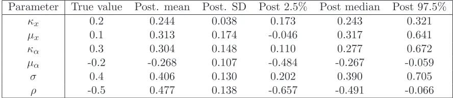
σ = 0.4,κx = 0.2,µx= 0.1, κα= 0.3 and µα=−0.2

The transformations required to construct an irreducible data augmentation scheme are

listed below. First we transform α toγ through

γt=

αt−α0

σ , 0≤t≤500,

αt=ν(γt, σ, α0) =α0+σγt.

Given γ, and for each pair of consecutive observation times tk−1 and tk (k = 1,2, . . . ,500)

on X, we transform as follows: First, we remove the term introduced from the leverage effect

Ht=Xt−

Z t

tk₋1

ρexp{ν(γs, σ, α0)/2}dWs, tk−1≤t≤tk,

and consequently we set

η(t) =

Z t

tk₋1

(1₋ρ)2exp_{ν(γs, σ, α0}ds.

Then,U and Z may be defined again from 12 and 13 respectively, but based onHrather on

X. The elements of the MCMC scheme areZ,γ,α0 and the parameters (κx, µx, κα, µα, ρ, σ).

We proceed by assigning flat priors to all the parameters, restricting κx, κα, σ to be

positive andρto be in (−1,1). The number of imputed points was set to 30 and 50, the length

of the overlapping blocks needed for the updates of γ was 2, and the relevant acceptance

rate 75% whereas the acceptance rate for X was 95%. Figure 3 shows autocorrelation plots

for the 2-dimensional diffusion’s (X, α)′ volatility parameters ρ and σ. There is no sign of any increase in the autocorrelation to raise suspicions against the irreducibility of the chain.

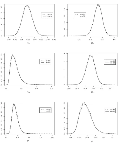
Figure 4 shows density plots for all parameters and both values ofm. These plots indicate a

sufficiently fine discretisation and a good agreement with true values of the parameters. The

latter is also confirmed by Table 1.

[Figure 3 about here.]

[Figure 4 about here.]

6

Application: US treasury bill rates

To illustrate the time change methodology we fit a stochastic volatility model to US treasury

bill rates. The dataset consists of 1809 weekly observations (Wednesday) of the 3₋month

US Treasury bill rate from the 5th of January 1962 up to the 30th of August 1996. The data

are plotted in Figure 5.

[Figure 5 about here.]

Previous analyses of these data include Andersen and Lund (1998), Gallant and Tauchen

(1998), Durham (2002), Durham and Gallant (2002), Eraker (2001), and Golightly and

Wilkinson (2006). Apart from some slight deviations the adopted stochastic volatility models

consisted of the following SDE.

drt = (θ0−θ1rt)dt+rtψexp(αt/2)dBt,

dαt = κ(µ−αt)dt+σdWt, (16)

with independent Brownian motionsB andW. In some cases the following equivalent model

was used:

drt = (θ0−θ1rt)dt+σrrtψexp(αt/2)dBt,

dαt = −καtdt+σdWt. (17)

We proceed with the model in (16), as posterior draws of its parameters exhibit substantially

less autocorrelation. In line with Gallant and Tauchen (1998) and Golightly and Wilkinson

(2006), we also set ψ = 1. Eraker (2001), Durham (2002) and Durham and Gallant (2002)

assume general ‘elasticity of variance’ ψ but their estimates do not indicate a significant

deviation from 1. By settingXt=log(rt), the volatility ofXtbecomes exp(αt/2). Therefore

the U−time for two consecutive observation times tk−1 and tk is defined as

η(t) =

Z t

tk₋1

exp(αt)ds,

and U andZ are given by (12) and (13) respectively . We also transformα toγ as before:

γt=

αt−α0

αt=ν(γt, σ, α0) =α0+σγt.

We applied MCMC algorithms based on Z and γ to sample from the posterior of the

parameters θ0,θ1,κ,µandσ. The time was measured in years setting the distance between

successive Wednesdays to 5/252. Non-informative priors were assigned to all the parameters,

restricting κ and σ to be positive to ensure identifiability and eliminate the possibility of

explosion. The algorithm was run for 50,000 iterations and for m equal to 10 and 20. To

optimize the efficiency of the chain we set the length of the overlapping blocks of γ to 10

which produced an acceptance rate of 51.9%. The corresponding acceptance rate for Z was

98.6% .

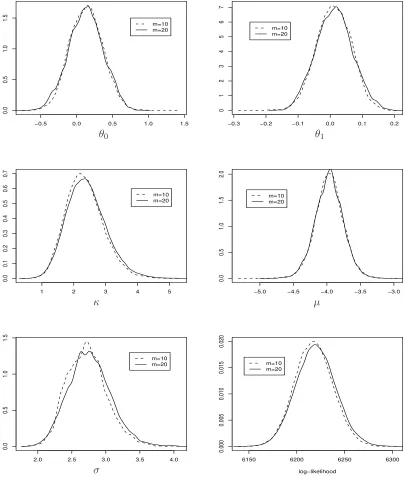
The kernel density plots of the posterior parameters and likelihood (Figure 6) indicate

that a discretisation from an m of 10 or 20 provide reasonable approximations. The

corre-sponding autocorrelation plots of Figure 7 do not show increasing autocorrelation in m, a

feature that would reveal reducibility issues. Finally, summaries of the posterior draws for

all the parameters are provided in Table 2. The parameters κ, µ and σ are different from

0 verifying the existence of stochastic volatility. On the other hand, there is no evidence to

support the existence of mean reversion on the rate, as θ0 and θ1 are not far from 0. The

results are in line with those of Durham (2002), Durham and Gallant (2002) and Golightly

and Wilkinson (2006).

[Figure 6 about here.]

[Figure 7 about here.]

[Table 2 about here.]

7

Discussion

Data augmentation MCMC schemes constitute a very useful tool for likelihood-based

infer-ence on diffusion models. They may not have the appealing properties of complete

elimi-nation of the time discretisation error (Beskos et al., 2006), or the closed form approximate

likelihood expressions of A¨ıt-Sahalia (2002), but nevertheless they give a satisfactory and

very general solution to the problem. However data augmentation schemes require careful

construction to avoid the degeneracy issues described at the beginning of this paper.

Here, we introduce an innovative transformation which operates by altering the time axis

introduce a novel efficient MCMC scheme which mixes rapidly and is not provibitively

com-putationally expensive. Our method is also easy to implement and introduces no additional

approximation error other than that included in methodologies based on a discretisation of

the diffusion path. Moreover it is general enough to include general stochastic volatility

models.

Further work will consider problems with state-dependent volatility and models which

involve jump diffusions, to which the methodology introduced here can be easily applied.

Fundamental to our approach here has been the introduction of a non-centered

parameter-isation to decouple dependence inherent in the model between missing data and volatility

parameters. However non-centered constructions are not unique, as illustrated by the choice

in the diffusion context between the state rescaling approaches of Golightly and Wilkinson

(2007); Roberts and Stramer (2001) and the time-stretching strategy adopted here. Clearly,

further work is required to investigate the relative merits of these approaches in different

situations.

8

Acknowledgements

This work was supported by the EPSRC grant GR/S61577/01 and by the Marie Curie

References

A¨ıt-Sahalia, Y. (2002). Maximum likelihood estimation of discretely sampled diffusions: a

closed form approximation approach. Econometrica, 70:223–262.

A¨ıt-Sahalia, Y. (2005). Closed form likelihood expansions for multivariate diffusions. In

preparation.

Andersen, T. G. and Lund, J. (1998). Estimating continuous-time stochastic volatility models

of the short term interest rate. Journal of Econometrics, 77:343–377.

Beskos, A., Papaspiliopoulos, O., Roberts, G., and Fearnhead, P. (2006). Exact and

compu-tationally efficient likelihood-based estimation for discretely observed diffusion processes

(with discussion). Journal of the Royal Statistical Society: Series B (Statistical

Methodol-ogy), 68(3):333–382.

Beskos, A. and Roberts, G. O. (2005). Exact simulation of diffusions. Ann. Appl. Probab.,

15(4):2422–2444.

Bibby, B. and Sorensen, M. (1995). Martingale estimating functions for discretely observed

diffusion processes. Bernoulli, 1:17–39.

Chib, S., Pitt, M. K., and Shephard, N. (2005). Likelihood based inference for diffusion

models. Submitted.

Durham, G. B. (2002). Likelihod based specification analysis of continuous time models of

the short term interest rate. Journal of Financial Economics. Forthcoming.

Durham, G. B. and Gallant, A. R. (2002). Numerical techniques for maximum likelihood

estimation of continuous-time diffusion processes.J. Bus. Econom. Statist., 20(3):297–316.

With comments and a reply by the authors.

Elerian, O. S., Chib, S., and Shephard, N. (2001). Likelihood inference for discretely observed

non-linear diffusions. Econometrica, 69:959–993.

Eraker, B. (2001). Markov chain Monte Carlo analysis of diffusion models with application

to finance. J. Bus. Econom. Statist., 19(2):177–191.

Gallant, A. R. and Long, J. R. (1997). Estimating stochastic differential equations efficiently

Gallant, A. R. and Tauchen, G. (1996). Which moments to match? Econometric Theory,

12(4):657–681.

Gallant, A. R. and Tauchen, G. (1998). Reprojecting partially observed systems with

applica-tions to interest rate diffusions.Journal of American Statistical Association, 93(441):10–24.

Golightly, A. and Wilkinson, D. (2006). Bayesian sequential inference for nonlinear

multi-variate diffusions. Statistics and Computing, 16:323–338.

Golightly, A. and Wilkinson, D. (2007). Bayesian inference for nonlinear multivariate

diffu-sions observed with error. Computational Statistics and Data Analysis. In press.

Gouri´eroux, C., Monfort, A., and Renault, E. (1993). Indirect inference. Journal of Applied

Econometrics, 8:S85–S118.

Heston, S. (1993). A closed-form solution for options with stochastic volatility. with

appli-cations to bonds and currency options. Review of Financial Studies, 6:327–343.

Hull, J. C. and White, A. D. (1987). The pricing of options on assets with stochastic

volatilities. Journal of Finance, 42(2):281–300.

Jones, C. S. (1999). Bayesian estimation of continuous-time finance models. Unpublished

paper, Simon School of Business, University of Rochester.

Jones, C. S. (2003). Nonlinear mean reversion in the short-term interest rate. The review of

financial studies, 16:793–843.

Kalogeropoulos, K. (2007). Likelihood based inference for a class of multidimensional

diffu-sions with unobserved paths. Journal of Statistical Planning and Inference. To appear.

Kalogeropoulos, K., Dellaportas, P., and Roberts, G. (2007). Bayesian inference for

correl-lated diffusions. In submision.

Oksendal, B. (2000). Stochastic differential equations. Springer, 5th edition.

Papaspiliopoulos, O. and Roberts, G. (2005). Retrospective MCMC for Dirichlet process

hierarchical models. Submitted.

Pedersen, A. R. (1995). A new approach to maximum likelihood estimation for stochastic

Roberts, G. and Stramer, O. (2001). On inference for partial observed nonlinear diffusion

models using the metropolis-hastings algorithm. Biometrika, 88(3):603–621.

Rogers, L. C. G. and Williams, D. (1994). Diffusions, Markov processes and martingales, 2,

Ito calculus. Wiley, Chicester.

Sørensen, H. (2004). Parametric inference for diffusion processes observed at discrete points

in time: a survey. International Statistical Review, 72(3):337–354.

Stein, E. M. and Stein, J. C. (1991). Stock proce distributions with stochastic volatility: an

analytic approach. Review of Financial Studies, 4(4):727–752.

Tanner, M. A. and Wong, W. H. (1987). The calculation of posterior distributions by data

List of Figures

1 Plots of a sample path forX,U and Z against their corresponding times for

σ=√2 andm= 7. Z equals 0 at time +_∞. . . 24 2 Updates of time scale parameters: For every proposed value of them, new

points are required and should obtained conditional on the stored points. . . 25 3 Autocorrelation plots for the posterior draws ofρandσ for different numbers

of imputed pointsm= 30,50. Simulation example of Chapter 3. . . 26 4 Kernel densities of the posterior draws of all the parameters for different

num-bers of imputed pointsm= 30,50. Simulation example of Chapter 3. . . 27 5 Weekly 3₋month US Treasury bill rate from the 5th of January 1962 up to

the 30th of August 1996. . . 28 6 Kernel densities of the posterior draws of all the parameters and the

log-likelihood for different values of imputed points m = 10,20. Example on Weekly 3−month US Treasury bill rates. . . 29 7 Autocorrelation plots for the posterior draws of the model parameters for

0 1 2 3 4

−1.0

−0.5

0.0

0.5

X−time

X

observed points imputed points

0 1 2 3 4

−1.0

−0.5

0.0

0.5

U−time

U

observed points imputed points

0 1 2 3 4

0.0

0.2

0.4

0.6

0.8

1.0

1.2

Z−time

Z

observed points imputed points

Figure 1: Plots of a sample path for X, U and Z against their corresponding times for

0.0 0.2 0.4 0.6 0.8 1.0

0.0

0.1

0.2

0.3

0.4

0.5

0.6

t

Z

stored points new points

0 100 200 300 400 500

0.0

0.2

0.4

0.6

0.8

1.0

Autocorrelation

m=30 m=50

0 100 200 300 400 500

0.0

0.2

0.4

0.6

0.8

1.0

Autocorrelation

m=30 m=50

Lag - σ

Lag - ρ

0.10 0.15 0.20 0.25 0.30 0.35 0.40 0.45 0 2 4 6 8 10 m=30 m=50

−0.5 0.0 0.5 1.0

0.0 0.5 1.0 1.5 2.0 m=30 m=50

0.0 0.5 1.0 1.5

0.0 0.5 1.0 1.5 2.0 2.5 3.0 3.5 m=30 m=50

−0.8 −0.6 −0.4 −0.2 0.0 0.2

0 1 2 3 4 m=30 m=50

0.0 0.5 1.0 1.5 2.0

0.0 0.5 1.0 1.5 2.0 2.5 3.0 3.5 m=30 m=50

−0.8 −0.6 −0.4 −0.2 0.0 0.2

0.0 0.5 1.0 1.5 2.0 2.5 3.0 m=30 m=50

κx µx

κα µα

σ ρ

0 500 1000 1500

0

5

10

15

Time in weeks from 5th January 1962

percent

−0.5 0.0 0.5 1.0 1.5 0.0 0.5 1.0 1.5 m=10 m=20

−0.3 −0.2 −0.1 0.0 0.1 0.2

0 1 2 3 4 5 6 7 m=10 m=20

1 2 3 4 5

0.0 0.1 0.2 0.3 0.4 0.5 0.6 0.7 m=10 m=20

−5.0 −4.5 −4.0 −3.5 −3.0

0.0 0.5 1.0 1.5 2.0 m=10 m=20

2.0 2.5 3.0 3.5 4.0

0.0 0.5 1.0 1.5 m=10 m=20

6150 6200 6250 6300

0.000 0.005 0.010 0.015 0.020 log−likelihood m=10 m=20 κ µ

θ0 θ1

σ

0 50 100 150 200 250 300 0.0 0.2 0.4 0.6 0.8 1.0 Autocorrelation m=10 m=20

0 20 40 60 80 100

0.0 0.2 0.4 0.6 0.8 1.0 Autocorrelation m=10 m=20

0 50 100 150 200 250 300

0.0 0.2 0.4 0.6 0.8 1.0 Autocorrelation m=10 m=20

0 50 100 150 200

0.0 0.2 0.4 0.6 0.8 1.0 Autocorrelation m=10 m=20

0 50 100 150 200

0.0 0.2 0.4 0.6 0.8 1.0 Autocorrelation m=10 m=20

Lag - σ

Lag - κ Lag - µ

Lag -θ0

Lag - θ1

List of Tables

1 Summaries of the posterior draws for the simulation example of Chapter 3 for

m= 50. . . 32 2 Summaries of the posterior draws for the stochastic volatility model of Weekly

Parameter True value Post. mean Post. SD Post 2.5% Post median Post 97.5%

κx 0.2 0.244 0.038 0.173 0.243 0.321

µx 0.1 0.313 0.174 -0.046 0.317 0.641

κα 0.3 0.304 0.148 0.110 0.277 0.672

µα -0.2 -0.268 0.107 -0.484 -0.267 -0.059

σ 0.4 0.406 0.130 0.202 0.390 0.705

ρ -0.5 0.477 0.138 -0.657 -0.491 -0.066

Table 1: Summaries of the posterior draws for the simulation example of Chapter 3 for

Parameter Post. mean Post. SD Post 2.5% Post median Post 97.5%

θ0 0.130 0.238 -0.347 0.132 0.589

θ1 0.013 0.057 -0.096 0.013 0.125

κ 2.403 0.620 1.319 2.360 3.745

µ -3.966 0.211 -4.384 -3.964 -3.547

σ 2.764 0.311 2.199 2.750 3.420