University of Twente
EEMCS / Electrical Engineering
Control Engineering
Design Space Exploration for
Fieldbus-based Distributed Control Systems
Matthijs ten Berge
M.Sc. Thesis
Supervisors
prof.dr.ir. J. van Amerongen dr.ir. J.F. Broenink ir. B. Orlic
August 2005 Report nr. 029CE2005 Control Engineering
EE-Math-CS University of Twente
iii
Summary
Development of embedded control systems at the Control Engineering chair takes a structured approach. It is supported by a toolchain consisting of both software and hardware tools that can be used in the various stages of the design process. The available tools range from modeling and simulation software to a hardware-in-the-loop simulator.
However, support for the implementation of control systems on distributed control systems is limited. Distributed systems consist of multiple processor nodes, interconnected by a fieldbus (or other communication solutions). As the fieldbus is part of the control loop, it will affect the behavior of the control system. With the existing toolchain, this effect is unknown until the complete control system is realized and measurements can be performed.
Implementation of embedded control systems can be complex and time consuming, as the implemented software solution must be validated on the actual target hardware. Embedded software is often difficult to debug, this depends on the debugging features of the development tools for the embedded platform.
The goal of this project is to design a new tool, which can be integrated in the existing toolchain, to aid in the verification and design space exploration during the implementation phase of a distributed embedded control system. This new tool, the Design Space Exploration (DSE) simulation environment, enables the simulation of a complete control system on a PC. It can be used during the implementation phase of the development process, and allows the designer to verify the correctness of the control system implementation and to choose the optimal parameters for all degrees of freedom (this is the design space exploration).
The DSE simulation environment is based on the Communicating Threads (CT) C++ library, which is an implementation of the Communicating Sequential Processes (CSP) language. This library supports a number of different platforms, which makes it possible to test software targeted at embedded hardware on a normal PC.
The DSE simulation environment incorporates a modified version of the TrueTime network simulator, allowing simulation of distributed systems. Support for network communication is further extended by the addition of Remote Channels to the CT C++ library. These Channels can be used to turn a normal CT Channel into a networked variant. In the Remote Channel concept a separation is made between parts that are specific to a single channel, to the communication hardware or to a single communication interface. This separation makes the addition of support for new hardware relatively easy, and it allows multiple channels to be routed over the same network interface, independent of the network hardware used.
To get the results from a simulation, a logging implementation has been made. Although this implementation is sufficient for use in simulations, it is not suitable for real-time logging. A logging concept is presented, which can be used both for real-time and simulation logging.
A demonstration setup, consisting of a distributed controller on two ADSP processor boards and the Linix plant, was simulated with the DSE simulation environment. This case shows how a simulation of a complete distributed control system can be constructed. Furthermore a smaller simulation setup was created, which shows an example of how the DSE simulation environment can be used for measurements on different communication protocols.
Samenvatting
De leerstoel Control Engineering gebruikt een gestructureerde benadering voor het ontwerp van embedded regelsystemen, welke wordt ondersteund door hardware- en softwaregereedschappen, die worden ingezet tijdens de verschillende stadia in het ontwerpproces. De beschikbare hulpmiddelen variëren van modelleer- en simulatiesoftware tot hardware-in-the-loop simulatoren.
Ondersteuning voor de implementatie van gedistribueerde regelsystemen is echter beperkt. Gedistribueerde systemen zijn systemen bestaande uit meerdere processors, die met elkaar verbonden zijn door middel van een veldbus (of andere communicatiemiddelen). Omdat de veldbus deel uitmaakt van de regellus, zal het gedrag van het totale regelsysteem erdoor worden beïnvloed. Met de bestaande verzameling van ontwerphulpmiddelen worden de gevolgen van deze beïnvloeding pas duidelijk nadat het hele regelsysteem is gerealiseerd en er metingen aan kunnen worden verricht.
De implementatie van een embedded regelsysteem kan complex en tijdrovend zijn, vooral doordat de resulterende softwareoplossing op het echte doelsysteem moet worden gevalideerd. Dit is zeer afhankelijk van de mate waarin de ontwikkelsoftware voor het doelsysteem hierin ondersteuning biedt.
Doel van dit project is om een nieuw gereedschap te ontwikkelen, dat geïntegreerd kan worden in de bestaande verzameling gereedschappen, waarmee de verificatie en design space exploration van een gedistribueerd embedded regelsysteem kan worden vereenvoudigd. Dit nieuwe gereedschap, de
Design Space Exploration (DSE) simulatieomgeving, maakt het mogelijk om een volledig
regelsysteem te simuleren op een PC. De simulatieomgeving kan gebruikt worden tijdens de implementatiefase van het ontwerp, waardoor mogelijkheden worden geboden om reeds tijdens deze fase de implementatie te verifiëren en optimale parameters te kiezen voor alle vrijheidsgraden in het ontwerp (dit is de design space exploration, ofwel de verkenning van de ontwerpruimte).
De DSE simulatieomgeving is gebaseerd op de Communicating Threads (CT) C++ bibliotheek, een implementatie van de Communicating Sequential Processes (CSP) taal. De bibliotheek ondersteunt een aantal platformen, waardoor het mogelijk wordt om software die bedoeld is voor een embedded processor te kunnen testen op een gewone PC.
De DSE simulatieomgeving gebruikt een aangepaste versie van de TrueTime netwerksimulator, waarmee het mogelijk is om gedistribueerde systemen te kunnen simuleren. De ondersteuning voor netwerkcommunicatie is verder uitgebreid door Remote Channels toe te voegen aan CTC++. Met deze Channels kan een gewoon kanaal eenvoudig worden omgezet in een netwerkvariant. In het Remote Channel concept is een scheiding aangebracht tussen de delen die specifiek zijn voor een enkel kanaal, voor de communicatiehardware of voor een enkele communicatie-interface. Door deze scheiding is het eenvoudig om ondersteuning voor nieuwe hardware toe te voegen. Bovendien kunnen meerdere kanalen dezelfde netwerkinterface gebruiken, onafhankelijk van de gebruikte netwerkhardware.
Om resultaten uit een simulatie terug te krijgen is de mogelijkheid om gegevens te loggen toegevoegd. De gebruikte implementatie biedt voldoende functionaliteit voor simulatie, maar is ongeschikt voor het loggen in real-time. Een alternatief concept, wat zowel in simulaties als in real-time situaties bruikbaar is, wordt daarom gepresenteerd.
Een demonstratieopstelling, bestaande uit een gedistribueerde regelaar op twee ADSP systemen en de Linix opstelling, is gesimuleerd met de DSE simulatieomgeving. Dit voorbeeld laat zien hoe een simulatie van een compleet gedistribueerd regelsysteem opgezet kan worden. Verder is een kleine simulatie gemaakt die laat zien hoe de simulatieomgeving ook voor eenvoudige simulaties kan worden gebruikt, bijvoorbeeld om metingen aan verschillende communicatieprotocollen uit te voeren.
v
Preface
This report forms the conclusion of my Electrical Engineering study at the University of Twente.
I am very thankful for everyone who helped me during this project. Special thanks go to Bojan Orlic, who has been of great help throughout the whole project. I also would like to thank Marcel Groothuis for his assistance, especially when numerous problems showed up during the development of the demonstration setups. The cooperation with Mark Huijgen has always been very pleasant, not only during this project, but also in several other projects throughout the study.
A final word of thanks goes to my parents for their unconditional support during my study.
Matthijs ten Berge
vii
Table of contents
1 INTRODUCTION ... 1
1.1 CONCURRENT SYSTEMS... 1
1.2 DESIGN TRAJECTORY... 1
1.3 DESIGN TOOLS... 2
1.4 OUTLINE OF THE REPORT... 3
2 DSE SIMULATION ENVIRONMENT... 5
2.1 MOTIVATION... 5
2.2 EMBEDDED SYSTEM SIMULATION... 6
2.2.1 Available simulators... 7
2.2.2 Basic assumptions and principles ... 8
2.2.3 Execution timing ... 9
2.3 DETAILED SIMULATION FRAMEWORK... 10
2.3.1 Continuous-time models... 10
2.3.2 The SimTimer... 12
2.4 THE LOGGER... 15
2.5 VARIABLES... 16
2.6 NETWORK... 16
2.7 CONCLUSIONS AND RECOMMENDATIONS... 16
3 NETWORK SIMULATOR ... 19
3.1 INTRODUCTION... 19
3.2 OVERVIEW OF THE TRUETIME NETWORK SIMULATOR... 20
3.2.1 Single run of the network simulator ... 20
3.2.2 Determining the next-run time... 22
3.3 CHANGES TO THE ORIGINAL TRUETIME NETWORK SIMULATOR... 22
3.3.1 Extraction of the network simulator core to pure C++ ... 22
3.3.2 Adapting the network simulator to fit into the DSE simulation framework ... 23
3.3.3 Interfacing the network simulator with the processor nodes ... 24
3.3.4 Some minor changes for improved usability ... 25
3.4 DEGREES OF FREEDOM... 26
3.4.1 Data Link layer type ... 26
3.4.2 Bitrate and transmit bandwidth fraction ... 28
3.4.3 Minimum frame size... 28
3.4.4 Packet loss probability... 28
3.4.5 Pre- and postprocessing delay ... 28
3.4.6 Collision window... 28
3.4.7 Slot time and node order... 28
3.4.8 Switch memory size, buffer type and overflow behavior ... 28
3.5 CONCLUSIONS AND RECOMMENDATIONS... 29
4 REMOTE CHANNELS ... 31
4.1 INTRODUCTION... 31
4.2 REMOTE CHANNEL CONCEPT... 31
4.2.1 Subdivision between RLD and NDD... 32
4.2.2 Network interface sharing and addressing... 32
4.2.3 Interface standards and data naming convention ... 33
4.3 PROTOCOLS AND OPTIONS... 34
4.3.1 Unreliable, asynchronous communication... 35
4.3.2 Rendezvous communication, object based acknowledgment ... 35
4.3.3 Rendezvous communication, block based acknowledgment... 36
4.3.4 Reliable, asynchronous communication (unavailable) ... 36
4.4 IMPLEMENTATION DETAILS... 36
4.4.1 Dynamic resizing of position numbers ... 36
4.4.2 Other configuration parameters ... 36
5 LOGGING...39
5.1 INTRODUCTION...39
5.2 LOGGING MODEL...39
5.2.1 Local logging ...39
5.2.2 Distributed logging ...40
5.3 DESIGN SPACE...40
5.3.1 Identifying objects ...40
5.3.2 Data generation...41
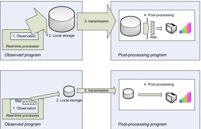
5.3.3 Filtering...43
5.3.4 Storage ...45
5.3.5 Transmission...50
5.3.6 Post-processing ...51
5.4 IMPLEMENTATION DECISIONS...51
5.4.1 Identifying objects ...52
5.4.2 Data generation...52
5.4.3 Filtering...52
5.4.4 Storage ...53
5.4.5 Transmission...53
5.4.6 Post-processing ...53
5.5 CONCLUSIONS AND RECOMMENDATIONS...54
6 DEMONSTRATION SETUPS ...57
6.1 INTRODUCTION...57
6.2 THE PLANT:LINIX...57
6.3 THE CONTROLLER...58
6.4 THE CONTROL LOOP...59
6.5 LOGGING...61
6.6 RESULTS...61
6.6.1 Comparison between 20-sim and the simulation environment ...61
6.6.2 Validation of the 20-sim model of the plant ...62
6.6.3 Variation of network parameters...63
6.6.4 Comparison between both Remote Channel rendezvous protocols ...65
6.7 CONCLUSIONS AND RECOMMENDATIONS...68
7 CONCLUSIONS AND RECOMMENDATIONS ...71
7.1 CONCLUSIONS...71
7.2 RECOMMENDATIONS FOR FURTHER RESEARCH...72
A REMOTE CHANNEL DETAILS APPENDIX...75
A.1 UNRELIABLE, ASYNCHRONOUS COMMUNICATION...75
A.2 RENDEZVOUS COMMUNICATION, OBJECT BASED...75
A.3 RENDEZVOUS COMMUNICATION, BLOCK BASED...77
A.4 WRITING A NETWORK DEVICE DRIVER...79
A.4.1 Deriving a class ...79
A.4.2 The constructor...79
A.4.3 The sendPacket function...79
A.4.4 Incoming data ...79
B 20-SIM MODEL APPENDIX ...81
1
1 Introduction
1.1 Concurrent
systems
As embedded systems become more and more complex, methods are needed to structure these systems. Defining a hierarchy and properly structuring the concurrency within this hierarchy can help dealing with the growing complexity.
In concurrent programming the task of the complete system is split up in blocks, where each block (process) has its own specific sub-tasks. Some of these blocks can run in parallel, others are to be run after their predecessor has finished or when a certain condition is met. The interrelationships between the blocks are denoted in a concurrency structure, which can be captured and analyzed via some formal method or process algebra, for instance in CSP (see below).
When the concurrency is not limited to single computer systems, but instead is spread over two or more computers, the term distributed computing is used. Where single-processor systems can only mimic parallel execution of software, for example by occasional switching between the processes, distributed systems can execute software truly in parallel. The different parts of a system need to communicate in order to achieve the desired system behavior. Therefore the communication between the participating computers is also assumed to be part of the distributed system. In most industrial applications all communication is performed over a fieldbus. Fieldbus is a generic term used to describe a common communication system for control systems or field instruments, hence its name. In this report the terms fieldbus and network are used interchangeably.
The Communicating Sequential Processes language (CSP) is a language in which concurrent systems can be described and analyzed algebraically (Hoare, 1985). Occam is a parallel programming language based on a subset of CSP and customized for a specific type of processors – transputers (Welch et al., 1993), which are nowadays obsolete. The CSP descriptions can be translated directly into Occam source code. Such a direct translation is however not possible into sequential languages like C, C++ or Java, as these languages lack a number of concepts.
Support for these concepts is added by using the Communicating Threads (CT) library (Hilderink et al., 2000). The CT library provides the necessary concepts in an object-oriented and structured way. Variants of the library are available for C, C++ and Java and are named accordingly: CTC, CTC++ and CTJ. The C++ version of the library has been the starting point for a rather drastic redesign (Orlic and Broenink, 2004). As this project is based on this redesigned version, only the C++ variant of the library is used.
1.2 Design
Trajectory
A specific design trajectory for embedded control systems development was defined in (Broenink and Hilderink, 2001). This design trajectory, as shown in Figure 1-1, consists of several phases.
Physical System modeling
Verification by Simulation
Control Law Design
Verification by Simulation
Embedded System
Implemen-tation
Verification by Simulation
Realization
Validation and Testing
In the first phase, the physical system modeling phase, models are designed that describe the dynamic behavior of the physical system. The results are verified by simulating the behavior of the model and comparing the simulation results with the physical system. This process can be iterative, by correcting the errors found during simulation in a new modeling cycle.
In the second phase, the control law(s) are developed. The result is again verified by simulation to check whether the desired control system behavior is achieved. Again this is an iterative process, which can partially be automated via iterative optimization functions such as curve fitting or error minimization.
In the third phase in the design process, the implementation phase, the designed control law(s) need to be converted into a software implementation. In case of a distributed system this phase also involves
process allocation, which is the distribution of the processes over the available processor nodes. In the implementation phase choices are made for the design options in the systems, such as the type of network, the needed bit rate and the assignment of priorities.
In the last phase the system is implemented on the target system(s). This can be done stepwise by using techniques like hardware-in-the-loop (HIL) simulation (Visser et al., 2004). In this phase the result can be validated, i.e. it must be assured that the requirements for the intended use of the control system have been fulfilled, for instance by testing the behavior of the completed system under various circumstances.
During the complete design trajectory the designer is exploring the design space. Every design contains a number of parameters, the degrees of freedom, which can be chosen by the designer. The complete design space consists of all possible combinations of these parameter values. Evaluating the effect on system performance of different combinations is called design space exploration, as (part of) the design space is searched for the optimal combination.
1.3 Design
tools
Some phases of the design trajectory are covered by design tools. Modeling of physical systems and design of control laws is covered by 20-sim. 20-sim is a modeling and simulation program developed by Controllab Products B.V. (CLP, 2002). The first two design phases can be covered completely by this program. Furthermore its code generation functionality has a role in the third phase. Another design tool is gCSP (Jovanovic et al., 2004). It provides a graphical language in which the concurrent structure of the design can be described. It can also generate code to implement this structure. The latest versions of gCSP now also support combining the generated blocks of code from 20-sim and gCSP into a usable program automatically. Simulation in the third design phase is not supported by existing tools. The final design phase is supported by HIL-simulation, where the plant is replaced by a combination of hardware and software that simulates the behavior of that plant. The realization of the control software is mostly supported by software development tools from the manufacturers of the target systems.
So far, all related previous projects implemented either simple control systems executed on single processor systems, or more complex distributed systems but with a fixed hardware topology and predefined process allocation. However, none of those projects did take into account a need for early design space exploration. Such a design space exploration, during the third phase of the design trajectory, is needed in order to identify optimal or suboptimal hardware and network topologies and mappings of software processes and communications to processing nodes and links prior to the actual implementation.
Chapter 1: Introduction 3
1.4 Outline of the report
To fill the gap in the tool support for simulation in the embedded system implementation phase, a simulation environment is developed. This simulation environment is also referred to as the DSE simulator, which stands for design space exploration, and is described in chapter 2 of this report. As mentioned, the networks are also part of a distributed system and need to be simulated. The part of the simulation environment that simulates these networks is presented in chapter 3.
In order to efficiently explore the design space for a distributed application that uses fieldbuses, one should be able to switch to different network types easily. The implementation of external channels in the CT library, which are used to let processes on separate computers communicate, did not provide this ability. Therefore a new implementation of these channels was developed. This new implementation, called Remote Channels, is described in chapter 4. Implementation details of the Remote Channels can be found in appendix A.
Obtaining results from a simulation, in whatever form, is an important aspect of a simulation. But also in an application running on the final target processor it can be important to observe parts of the program. These data-gathering activities all fall under the denominator of Logging and are described in chapter 5.
In order to test the simulation environment with a real example, a setup has been build using two Digital Signal Processor (DSP) boards from Analog Devices and a hardware plant, called Linix. This setup and its simulation with the new simulation environment are presented in chapter 6. This chapter also contains results of the performance measurements on the Remote Channel protocols. The model of the control system is shown in appendix B.
5
2 DSE Simulation Environment
2.1 Motivation
The design trajectory for embedded systems is shown again in Figure 2-1. Some tools that can be used in the phases are indicated. It is assumed that 20-sim is part of the toolchain and that it will be used during the first two design phases. 20-sim can be used for both the design and simulation steps in these phases.
The design trajectory shown in the previous chapter (see Figure 1-1) also shows a verification by simulation during the implementation phase of the design. Besides some formal checking methods, the toolchain however does not provide means for simulation during this phase. The simulation environment presented in this chapter is meant to fill this gap. Some arguments why such a simulation environment is needed are given below.
Physical System modeling Verification by Simulation Control Law Design Verification by Simulation Embedded System Implemen-tation Verification by formal checking Realization Validation and Testing 20-Sim Code generation, gCSP Target, HIL
Figure 2-1 Design trajectory for embedded control systems
All embedded system design phases should provide simulation support
Simulation in the physical system modeling and control law design phases (see Figure 2-1) can be useful to verify the correctness of physical and control system models and its parameters. It is possible to generate code from the obtained models, for instance by using the code generation features of 20-sim. The generated code can be customized for a specific hardware platform by defining template files containing platform specific code, which is for instance done for the ADSP platform in (Mocking, 2002). The simulator in these design phases is however not capable of verifying the generated
software implementation of a model in the context of the given hardware platform.
The embedded system implementation phase is currently only supported by the 20-sim code generation and a tool for structuring concurrency, the gCSP tool (Jovanovic et al., 2004). In the current state of development, the gCSP tool can aid in entering a design graphically and it can generate code from this design. Code blocks generated from 20-sim can be embedded using process wrappers, and supplemental processes can be added. The concurrency structure of the design can be entered by defining compositional and communication relationships between processes and grouping them into constructs. Code for the executable, as well as the code for formal CSP model checking, can be generated for the given designed process architecture. No simulation or analysis, other then formal checking for concurrency problems, can be performed by the gCSP tool as it is now.
The embedded system realization phase already deals with the real target hardware. Another project, focused on this phase (Visser et al., 2004), exists, that deals with the implementation of HIL
provide valuable feedback to the designer, it is a kind of post-game approach, in the last phase of the design trajectory.
An overall system simulation, capable of capturing the influence that embedded system implementation exerts on the behavior of the overall system, is also needed in an earlier phase of the design trajectory. The implementation phase is the earliest phase where this overall system simulation can be performed.
Validation and Testing on the target is expensive
Testing the generated code and its surrounding software is very well possible on the real target, as the software is ultimately meant for that target. Of course the hardware must already be available, which is not always the case. Design iterations on the real target can come at high costs. When changing a parameter in the software, a lot of time is spent on recompiling and downloading the new code into the target.
Changing a parameter like the type of fieldbus on a real target is another example of design space exploration at high costs: changing the network type does not only require software changes, but also changes in hardware, which costs both time and money. This can range from simply exchanging a hub for a switch to a full redesign of the target with different hardware components. As a general rule it can be assumed that design changes in a later phase of the design process are more expensive than in earlier phases, see for instance (Douglass, 2003).
In-target debugging can be hard
Depending on the target, it can be difficult to debug the software just by running it on the target. Some targets provide good debugging support: PC104 stacks running Linux for instance provide networking, a login console and a debugger installed. Other targets do not provide debugging support at all (mostly microcontrollers) or at high costs. These costs can be both time (stepping through the code of an ADSP-21992 takes about two seconds for each step) and money (for example in-circuit device emulators for microcontrollers).
2.2 Embedded system simulation
With the embedded system simulation environment an extra sub-phase in the design trajectory is introduced (see Figure 2-2). Its intended place in the design trajectory is at the embedded system implementation phase. It can be expected that in the future the gCSP tool will be enhanced with
Physical System modeling Verification by Simulation Control Law Design Verification by Simulation Embedded System Implemen-tation Verification by formal checking Realization Validation and Testing 20-Sim Code generation, gCSP Target, HIL Verification by Simulation Simulation Environment
Chapter 2: DSE Simulation Environment 7
support for this simulation framework. However, since the simulation framework is being developed in parallel with gCSP tool, it is directly building upon the code obtained by 20-sim code generation.
After code is generated from the simulation model, it can be combined with the other software components, just as if the implementation is to be tested on the target system. But instead of running on the target, the software can run in a simulated environment on a normal PC. The simulator environment provides a number of components with functionality needed for a simulation run. These components are discussed in this chapter. The term ‘simulation environment’ is more appropriate than ‘simulator’, as the resulting executable runs independently, as opposed to a simulation model or script, which is executed by a simulator. As such, the developed components do not make up a simulator, but they create an environment in which the simulation can be executed.
20-sim model of Plant 20-sim model of Controller Code generation Code generation templates Source code for Controller Source code for Plant Combine Source code for other controller tasks Combine C/C++ Compiler for PC C/C++ Compiler for target Simulation executable Target executable CT library DSE simulation environment components
Figure 2-3 Steps to create executables for simulation or for the target
2.2.1 Available simulators
A number of simulators and related tools for real-time and control system co-design is already available in research communities. A good overview is given in (Henriksson et al., 2005). This project is especially interested in simulation of distributed systems, with a focus on the influence of the networks. Therefore, especially appealing was to investigate whether existing network simulators can be reused. Several research projects such as ‘ns2’, a network simulator from the VINT project (VINT, 2005), ‘Real’, a network simulator from Cornell University (Keshav, 1997) and TrueTime (Henriksson and Cervin, 2003) were investigated.
The design of a new simulation environment from scratch however had some important advantages: Simulations are C++ programs
uses a combination of Matlab code, Simulink models and MEX functions. Furthermore, the resulting executable can run stand-alone, with little overhead compared to scripted (interpreted) simulators. It is possible to use existing C++ development tools, debuggers and profiling tools. The latter can for instance be used to get insight in how the processing load is balanced over the nodes.
Coupling with 20-sim
A tight coupling with 20-sim is necessary to easily move on from the model-based simulation design phase to the code-based simulation. The code-generation tool of 20-sim can provide this coupling. Use of CSP
The simulation environment is based on the CT C++ library, an implementation of the CSP theory (Hoare, 1985). In the current design flow, CT C++ is already often used to finally implement the software. By using it also in the simulation environment, the transition from source-code-based simulation to verification on the target will be smooth. Because CT supports several platforms, development can be done on the platform of choice. Thanks to the structure of a CSP program, it is very easy to assign processing tasks to a different processor node, just by moving part of the process hierarchy to a different location on the tree and replacing local channels with remote channels or vice versa.
2.2.2 Basic assumptions and principles
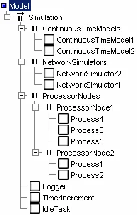
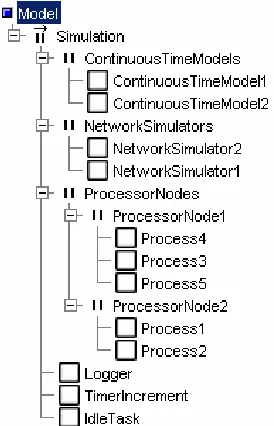
The simulation is based on the idea that a complete distributed system can be represented by adding higher layers to the existing process hierarchy (see Figure 2-4 and Figure 2-5). That part of the application that should be executed on one single node is wrapped in a process. As this process represents the complete node, it is named after this node (ProcessorNode1 and ProcessorNode2 in the example shown in the figure).
Networks are also represented as processes (NetworkSimulator1 and NetworkSimulator2 in the example). All communication channels that were local to a certain node remain local inside the wrapper process of that node. Instead of communicating with network interface hardware, all remote communication channels are now communicating with the processes that represent the network(s). The main idea is to keep all executable code intact and only add additional processes to simulate the networks.
Figure 2-4 Typical simulation layout
Chapter 2: DSE Simulation Environment 9
the whole system. The complete system also contains some extra components, such as the Logger and the TimerIncrement. The Logger provides data logging functionality and the TimerIncrement is part of the timing implementation of the simulation. These components are discussed in detail later, in section 2.3.2 and 2.4.
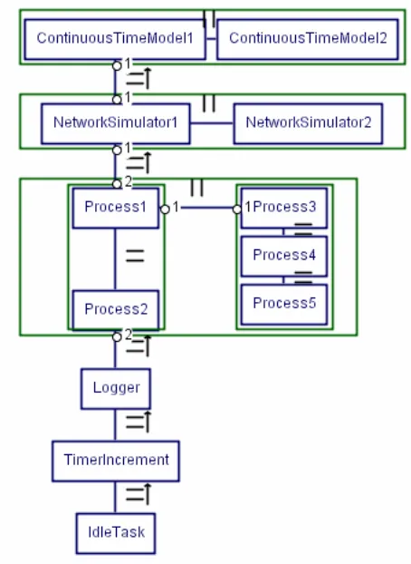
Figure 2-5 Simulation layout block diagram
Since focus is put on the influence of networks on distributed system simulation, the decision was made to assume that major overhead is induced by network delays and that the computation overhead is negligible compared to any network delays. Due to significant difference in speed between processing and communication devices, this assumption is a valid first approximation for most real life systems.
2.2.3 Execution timing
As stated in the previous section, the network delays are assumed to be large compared to the execution time of the code. However, for simulations with relatively fast networks, or no networks at all, the execution time of the processor nodes should be taken into account. As an exception, when both inputs and outputs of the code blocks are timed, the code execution time will not influence the behavior of the system: reading the inputs and updating the outputs then occurs at fixed intervals, independent of calculation delays.
The reason that the code execution time is not part of the current DSE simulation environment is twofold.
Cooperation with the CT scheduler is also needed, because a distinction must be made between processes on different or on the same processor node: processes on different nodes can run truly in parallel, while processes on the same processor node cannot run in the time already consumed by other processes on that same node. The Channels also need to be aware of the timing issues: when determining the order of arrival of reader and writer, the simulation time of both reader and writer must be taken into account. Possibly the concept of the TrueTime kernel simulator (Henriksson and Cervin, 2003) can be used.
- Furthermore it requires the execution time of all relevant code blocks to be measured or estimated. Measurements cannot be done on a random desktop PC; they have to be done on the real target processor(s), as the architecture, instruction set and execution speed will most likely differ. Measuring the execution time is hindered by instruction and data caching, interrupts and conditional branching in the code, because they all influence the execution times. On the other hand, estimation of execution times requires building complex detailed models for every target hardware platform.
As a result of the untimed code execution, it is not possible to have for instance a process with an endless loop in a processor node construct. Such a process will run forever, causing the TimerIncrement process never to be reached. As a workaround for this kind of situations, one could make such a process timed, by letting it block on a timer channel on every iteration of the loop.
2.3 Detailed
Simulation
framework
The DSE simulation is based on a CSP hierarchy tree, like the example shown in Figure 2-4, and implemented using the CT C++ library. The way the different components are arranged in the main PriPar construct ensures proper timing of the simulation, as will be shown in section 2.3.2, Simulation process and its timing.
2.3.1 Continuous-time models
On top of the hierarchy are the continuous-time models. These are the numerical models representing the physical process (plant) which will be controlled by the embedded system. As the simulation is based on discrete-time simulation, the continuous-time models are approximated by discretizing them at sufficient small time steps. As a rule of thumb, the time steps of the discretized model should be ten times as small as that of the other, discrete, components in the system (Groothuis, 2004). In this project however, a more accurate method was applied. Instead of updating the states and rates of the plant much faster than those of the other, discrete components, the states and rates are updated only when that is needed according to the plant dynamics or as result of actions of other discrete components.
In the examples, discretizing is performed by the 20-sim code generation feature, based on Euler’s method. This method normally produces models with a constant time step. Besides the normal model calculations at fixed time steps, extra calculations can be performed when it seems appropriate. Typically this will be the case when a discontinuity in the model is expected, for instance when a discrete controller updates an input of the model. The method of triggering these extra calculations is addressed in section 2.3.2: SimTimerChannel advanced features.
Variable-step Euler discretizing
Ordinary Euler discretizing (see Figure 2-6) works by determining the rate-of-change of the model states at a time t0. These rates are multiplied by the configured time step size tstep and added to the
states at t0 to obtain an estimate of the states at t2 (=t0 + tstep). Within the interval t0…t2 the rates are
assumed to be constant. Because of the fixed step size, all calculations to determine the states at t2 can
already be performed while the simulation is still at t0. Depending on the dynamics of the model, the
Chapter 2: DSE Simulation Environment 11
However, when such a model is combined with for instance a discrete model running at a different time step, the inputs of the continuous-time model could change drastically at time t1 (somewhere
between t0 and t2, see Figure 2-7), due to the discrete model updating its outputs. At t1, the estimated
states need to be updated for the partial step between t0 and t1, and the rates need to be recalculated for
the new situation.
t
0t
2st
a
te
actual
estimate
Figure 2-6 Euler discretization
As the time step t0-t1 is not known in advance, it is impossible to calculate the next states while still at
time t0. The only thing that can already be calculated then is the rate-of-change. At time t1, the actual
time step that is taken is known and can be used to calculate the states at t1. After updating the states,
the new rates can be calculated. This is also how the simulation wrapper around the continuous-time models implements the variable-time Euler method (this implementation can be found in the file linixplant/linixplant.cpp in the linixsim example directory).
t
0t
2st
at
e
actual
estimate
t
1Figure 2-7 Recalculating the rate at a discontinuity
2.3.2 The SimTimer
As already mentioned, the DSE simulation uses discrete time steps. One global object, the SimTimer, is used to keep track of this simulation time. The SimTimer does not directly show up in the process hierarchy (Figure 2-4), as it is a passive object. Instead, the active object TimerIncrement, which is a process and as such does show up in the process hierarchy, is used to execute the SimTimer’s functionality.
Processes are not allowed to use the SimTimer directly. As CSP only allows processes to communicate using channels, the processes should create a channel to the SimTimer. This
SimTimerChannel encapsulates the interface to the timer (see Figure 2-8).
Process
Process
SimTimer Channel
SimTimer Channel
SimTimer object TimerProcess
Figure 2-8 SimTimerChannels
The SimTimer should be an active object, as in CSP Channels should have processes (active objects) on both sides. The SimTimer is however a passive object, ‘borrowing’ the thread of control from the IncrementTimer process (see TimerProcess in Figure 2-8) This separation, which could cause some confusion, has a reason. It makes it very easy to change the ‘source of execution’ (i.e. where the SimTimer borrows its thread of control from) to for instance a different process, a hardware interrupt function or an operating system callback function. A purpose for this is explained in section The SimTimer in real applications, further on this section.
SimTimerChannel basic features
Reading from the SimTimerChannel will return the current simulation time. This communication will never block, as such it can be seen as a read from an overwrite channel.
Writing to the SimTimerChannel can however be a blocking communication. Blocking occurs if the written time value lies in the future (with respect to the simulation time). The writing process will then block on the SimTimerChannel until the requested simulation time has become present. If, on the other hand, the written time value is already in the past, the channel communication will not block, but return immediately.
DSE simulation processes and its timing
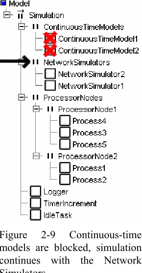
The blocking behavior of the SimTimerChannel is utilized by organizing all processes in a PriPar construct: the processes with highest priority, the continuous-time models, will initially be the first processes allowed to run. They will perform a model calculation step and then write the time value of their expected next run to their SimTimerChannels. As this requested time is in the future, the channels will cause the continuous-time model processes to be blocked. Now the processes with the next highest priority, the network simulators, will be executed (see Figure 2-9). Similarly to the continuous-time models, the network simulators will also do a simulation step and block on the SimTimerChannels.
Chapter 2: DSE Simulation Environment 13
situations (except when there are external interrupts) this situation is called a deadlock. But in the simulation there is still a process left that is runnable: the TimerIncrement process.
Figure 2-9 Continuous-time models are blocked, simulation continues with the Network Simulators
The TimerIncrement process requests the SimTimer to increment the simulation time. Out of all requested times on the blocked SimTimerChannels, the SimTimer selects the one that is most near, i.e. the smallest time increment. It increments the simulation time to this new value. The SimTimerChannels which now meet the current time are unblocked, the others are left blocked.
Basically this is the way passage of time is often expressed in simulation environments. First, all processes are allowed to execute without real passage of the time. Once all processes are blocked on either time channels or communication events, the time will be incremented to the next valid point. As the unblocked processes have a higher priority than the TimerIncrement process, program execution will continue with those.
This was the reason for introducing a PriParallel instead of a Parallel composition. The TimerIncrement process should be preempted after each time update and will not make extra time increments until all other processes are blocked again. In order for this construction to function properly, the TimerIncrement process should allow a context switch to take place after each timer increment. In the CT library framework this can be done for instance by using a sequence of calls to the enterAtomic and exitAtomic functions or by using the yield function. If this is not done, or if for instance the PriPar’s implementation is not correct, the TimerIncrement process will remain the active process. It will then step through the complete simulation time in one run, leaving the other processes no chance to do their work.
SimTimerChannel advanced features
The first method is by using a SimTimerChannel earlyRelease. Any process, except for the blocked process itself of course, can earlyRelease a SimTimerChannel. The channel is unblocked immediately and, depending on the relative priority of the processes, the unblocked process might be executed immediately. As the current Channel interface in the CT C++ library does not allow return values for channel operations, it is not trivial to let the process know that is was earlyReleased. Besides obtaining this information by changing the Channel interface definition in the library, or by using the exception mechanism, the process can also perform a read on the SimTimerChannel to obtain the current time, and compare it with the time it had requested in the write operation.
The earlyRelease method is used in the RemoteLinkDriver (see also chapter 4) to handle incoming packets and timeouts: first a packet is sent, and then the process writes the packet timeout time to its SimTimerChannel. If no acknowledging packet arrives, the time specified in the SimTimerChannel will eventually expire and the sending process is released, knowing that a timeout has occurred. On the other hand, if an acknowledgement packet is received, the SimTimerChannel will be earlyReleased, allowing the incoming packet to be processed immediately.
The second method is by using a globalEarlyRelease. A process can request the SimTimer to iterate over all available SimTimerChannels to see whether it can earlyRelease them. On creation of a SimTimerChannel, one has to specify explicitly that the channel is susceptible to a globalEarlyRelease. The SimTimer will skip channels that do not specify this property, and channels that are not blocked.
This method is used to perform the extra simulation steps in continuous-time models. Any time when a discrete model delivers a new input value to a continuous-time model, is should request a globalEarlyRelease. The continuous-time models will then be interrupted. They read the current time and perform a model calculation based on this time.
The SimTimer in real applications
Despite its name, the use of the SimTimer is not restricted to simulations. It can also be used in real (real-time) applications. On the side of the processes nothing needs to be changed, as the SimTimerChannel forms an abstract, platform independent interface to the timer. Only the software component which increments the timer needs to be changed.
Incrementing the time is no longer performed by a process, as in the DSE simulation, but by a real timer implementation. The SimTimer can for instance be incremented from a hardware timer interrupt service routine or from a callback function which is called by the Windows multimedia timer. The SimTimer object is now not longer a passive object, but it has its own thread of control, namely the thread that executes the interrupt or callback function.
Instead of incrementing the timer up to the nearest time, the timer is now incremented with fixed time steps, representing the step size of the timer source. So if, for instance, a hardware timer is running at one kilohertz, the SimTimer is incremented a millisecond each step. It is even possible to update the timer from more than one source of time; as long as those sources do not interrupt each other (interrupt nesting). In this case, the routines should update the SimTimer using absolute time values instead of steps relative to the previous value.
An example of the use of the SimTimer in a real application is the Linix demonstration setup, which will be discussed in chapter 6. It uses one of its hardware timer modules to generate an interrupt. The SimTimer gets updated from that interrupt routine. The timer is used via two SimTimerChannels, one to wait for the next run of the controller model, the other to provide the Logger with values for its timestamps.
Units of time
Chapter 2: DSE Simulation Environment 15
has the advantage that it scales to the needed time range, i.e. it is both possible to use very small time units (like microseconds) or very large time units (like hours) with full precision. A combination of both small and large units however, causes rounding errors to occur. This disadvantage has to be taken care of, for instance by never comparing two time values to be equal. Instead, they should be compared to be ‘almost equal’, thereby allowing a small percentage of deviation.
The SimTimer can also be configured to use a different type as its time unit, namely an integer. This setting can not be combined with the network simulators or continuous-time models without some modifications. For real applications however it can be somewhat more convenient. The unit of time can for instance be chosen to correspond to one hardware timer tick, i.e. the timer interrupt routine increments the SimTimer by one. Rounding errors like with floating point numbers do not occur. Instead, a timer overflow can be expected, but this can be handled easily.
The Linix demonstration setup mentioned already will work with either configuration. Depending on the configured time type, it chooses the correct step size to update the timer and to wait for the next model run.
2.4 The
Logger
The Logger is used to transfer results of the simulation to an external data processing application. It is discussed in detail in chapter 5. The low-priority position of the Logger in the simulation hierarchy (see Figure 2-4) might seem somewhat awkward, as storing the results has a high priority in simulation, i.e. in a simulation it is more important to store all results than to run the simulation at high speed. However, with an eye on real-time execution on the target, where timely execution is of higher priority than logging all results, it is a logical choice.
First consider the simulation case. At a certain time the processes in the tree are executed. They will generate some log information, which will be stored in a buffer. No data can be transmitted yet, as the Logger will not get scheduled because of its low priority. At a certain point all processes are finished with this iteration and they are all blocked. Now the Logger will be executed and it will transmit the entire contents of the log buffer to the outside world (more on this in chapter 5). Only when all data has been sent, it will block and give over control to the TimerIncrement process, which will initiate a new time step.
Provided that the log buffer is large enough, which will not pose any difficulties as no significant memory limitations exist on most development machines, this process layout can guarantee that all data is logged, at the cost of speed. Furthermore it can guarantee that, when compared to the real target execution, the order of DSE simulation execution is not distorted because of the influence of the Logger.
Now consider the real target case. As mentioned before, there is no TimerIncrement process in this situation. Again, at a certain time the (real-time) processes are executed. Log information is accumulated in the log buffer. As soon as all processes are done, the Logger is scheduled and it will start transmitting the log data. When it is done, control is passed to the Idle task, which typically is a process doing just nothing. At the next hardware interrupt, some or all of the channels will be unblocked (whether these are timer channels or remote channels), and process execution will continue, and new log data is generated.
Summarizing, this process layout allows the Logger to completely execute once at every time point in the simulation case, while the same layout causes it to only run at ‘idle’ priority in the real-time case.
2.5 Variables
Although the code simulation runs on another platform than the final target, it should ideally behave the same for proper simulation and debugging. The behavior should also be the same for all possible target platform implementations as much as possible. One of the main incompatibilities of different targets is the difference in variable types. Consider for instance a type very commonly used in C++, the pointer. On a standard PC platform with a common compiler, a pointer will probably take 32 bits of storage. On an Analog Devices ADSP however, it will have a size of only 16 bits. And finally on the IA-64 architecture it would probably take 64 bits.
This problem is tackled by defining variable types that have a fixed size on all platforms. The implementation of those variables will thus be dependent on the platform used, but their use is platform independent from the applications point of view. Currently the most common variable types are defined for a number of platforms. Unfortunately, the 64-bits variables are not implemented on ADSP, as this platform does not support 64-bits arithmetic at all. All operations on those variables then need to be emulated in software, which requires quite some work.
The defined variable types also have support for logging built in. When this support is enabled, a variable of one of these types will generate a log message as soon as it is created or deleted or its value is changed. Logging is described in detail in chapter 5.
2.6 Network
The network simulators have a higher priority in the DSE simulation tree hierarchy (Figure 2-4), as in practice the transport and delivery of network packets is independent of the software that runs on the processor nodes.
Two separate networks are completely independent in reality. In the simulation this is represented by running every network in a separate process, concurrently with the other network representing processes. In most situations only one network is used, so the parallel construct of network simulators is reduced to a single network simulator process. The network simulator is treated in chapter 3.
As an interface between the network simulators and the processes on the processor nodes, Remote Channels are provided. Remote Channels can be used instead of local channels, between two processes. They can both be used in the simulation as on real hardware. Remote Channels and the communication protocols they support are treated in chapter 4.
2.7 Conclusions and recommendations
The designed DSE simulation environment extends the development toolchain by providing the ability to perform simulations of the complete embedded system during the implementation phase of the design trajectory. This allows the designer to investigate the consequences of design choices during this phase, instead of having to wait until the realization phase. This makes it possible to analyze the consequences of design decisions early in the design process, allowing for multiple design iterations (exploration of the design space) without high costs.
The simulation environment integrates into the existing toolchain by using the code generation functionality of 20-sim. The integration could however be improved, as it still requires quite some manual programming work to set up a simulation. As far as the generated code from 20-Sim is concerned, most manual intervention is involved in connecting the inputs and outputs of a model to the rest of the simulation. This work might be automated by extending the functionality of the
Chapter 2: DSE Simulation Environment 17
Using the gCSP design tool to design the concurrency structure and to automatically connect the processes using local or remote channels would also decrease the amount of manual work involved. Currently all network nodes, network node- and link-ID’s (see also chapter 4) need to be numbered manually, which is a tedious task that can easily be (semi-)automated by using gCSP.
19
3 Network
Simulator
3.1 Introduction
In order to be able to simulate distributed systems, the communication between the nodes in such a system needs to be available in a simulation environment as well. The communication is assumed to take place over one or more networks, so a network simulator component is needed.
A number of network simulators already exist. With respect to the data routed over those simulated networks and their abstraction layer, they can be sorted in two categories:
Network simulators with parameterized data flows
In these simulators, the content of the data flows is characterized by a number of parameters, such as the stochastic distribution of the packet size, the number of packets and the source and destination nodes. No real data is transmitted over the simulated network.
This type of simulator often works on a somewhat higher communication layer, like for instance the Transport Layer and may be useful to investigate for instance the effects of routing, queuing policies, flow-rate protocols and topology on network delays. The International Standard Organization's Open System Interconnect model (see the ISO/OSI documents in ICS section 35.100) contains a division of the communication model in layers. Examples of this type of simulator are ‘ns2’, a network simulator from the VINT project (VINT, 2005) and ‘Real’, a network simulator from Cornell University (Keshav, 1997).
Network simulators with real data flows
These simulators transfer real data over the simulated network. The sending network nodes will need to provide this data; the network simulator delivers it to the receiving nodes, which can then process it. Such simulators generally work at a lower network layer, like the Data Link layer. They handle media access, collision detection and retransmits. An example of this type of simulator is TrueTime (Henriksson and Cervin, 2003).
For the distributed simulation, a simulator of the second type is most useful, for two reasons.
- The first reason is that embedded controllers often do not use a standard network protocol stack like a TCP/IP stack. Instead, the software communicates directly with the network interface hardware in such cases to send and receive packets. The communication protocols are then implemented in the application software itself. In order to simulate such a situation with a Transport Layer simulator, the simulator must first be taught the behavior of the non-standard protocol used. A simulator based on the Data Link layer on the other hand will be able to simulate both default protocols and user-defined protocols, as in both cases the behavior of the Data Link layer will remain the same.
- The second reason is that it is really useful to work with real data over the network. Simulating a distributed control system differs from for instance research of large networks, where single users are often anonymous and where the data they send is not relevant. In a distributed control system, the identity and behavior of the different network nodes is generally known and the data that is sent across the network can influence the behavior of the nodes. A simulator which does not transport real data could be used, but then some arrangement must be made to temporarily store the transferred data, so the receiving node can pick it up again. This requires some software administration, which is not needed in case the simulator can transfer the data itself.
TrueTime provides support for most Data Link layer types in use nowadays, such as CSMA/CD used in Ethernet, CSMA/AMP used in CAN networks and Round Robin used in Token Ring networks. A complete enumeration of all supported Data Link layer types, together with a description, can be found in section 3.4.1.
3.2 Overview of the TrueTime network simulator
The TrueTime network simulator is primarily based on packets and queues, which are represented in C++ using objects and linked lists. A packet will always belong to only one queue (an exception to this is a broadcast packet, which will be assigned to the queues of all receiving nodes).
The computers attached to the network are represented by NWnode objects. These objects contain the queues and information about the node. Each NWnode has its own full set of queues, unique to the network to which the node is attached. If the node is connected to multiple networks, it also owns multiple sets of queues. All data sent by a particular node to a particular network will always be added to the queue set belonging to that node and corresponding with that network.
3.2.1 Single run of the network simulator
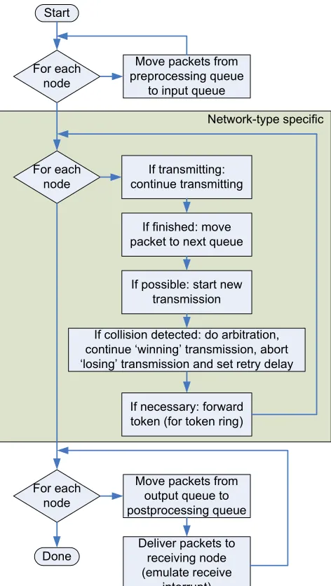
The way a data packet travels through the network simulator is depicted in Figure 3-1, while Figure 3-2 shows a flowchart of a single run of the network simulator. These figures depict what is performed in a single run of the network simulator.
Preprocessing queue
Input queue
Optionally: switch queue
Output queue
Postprocessing queue Driver
Application
Preprocessing
delay Wait, collision or back-off
Transmission succesful
Postprocessing delay
Driver Application
Figure 3-1 Packet flow through the network simulator
The contents of a data packet in the simulation are determined by the application that wants to transmit, just as in a real application. The application hands this data to a network interface driver. But instead of placing the packet in the transmit buffer of a network interface hardware, the packet is now placed in the preprocessing queue belonging to the sending node.
Packets will wait in the preprocessing queue for some period determined by the preprocessing delay
parameter. This parameter can be used to mimic the delay between the moment the application offers a packet and the moment a first transmission could be attempted. This can incorporate both software and hardware delays, which can for instance be caused by the operating system, the network driver and the network interface hardware. After this delay the packet is placed in the input queue.
The input queue will hold packets until they are fully transmitted. Only the topmost packet in the input queue is transferred in the single simulation transmission. All other packets will remain untouched until they are on top (this allows for sorting the queue, see section 3.3.4). Packets will remain waiting in the input queue until the node is allowed to send. How long packets will have to wait in the input queue depends on the length of the queue and the relative priorities of other packets, but also on the network protocol used.
Chapter 3: Network Simulator 21
back-off time is calculated. This is the time during which the node is not allowed to send. The packet remains in the input queue during back-off.
In full-duplex switched-mode networks collisions in the usual sense will not occur. However, when the switch memory is full, packets can either be dropped, or the switch can signal a collision, in which case the transmitter will retry after the back-off time. This behavior of the network switch is configurable and is explained in detail in section 3.4.8.
If transmission was successful, the packet will either be moved to the switch queue or the output queue
of the receiving node, depending on the configured network type. From the switch queue a packet will be delivered to the output queue without collisions.
Packets in the output queue will remain there for a configurable period, the postprocessing delay. This delay is comparable to the preprocessing delay, but now for incoming packets (note that the term ‘output queue’ can be misleading, as the output of the network simulator is the input for the nodes). After this delay the packets are moved to the postprocessing queue, where the application can pick them up.
Start
Move packets from preprocessing queue
to input queue For each
node
For each node
If transmitting: continue transmitting
If finished: move packet to next queue
If possible: start new transmission
If collision detected: do arbitration, continue ‘winning’ transmission, abort ‘losing’ transmission and set retry delay
If necessary: forward token (for token ring)
Move packets from output queue to postprocessing queue For each
node
Deliver packets to receiving node (emulate receive
interrupt) Done
Network-type specific
Figure 3-2 Program flow of the network simulator
now executed by the thread of the network simulator instead of a hardware interrupt thread. As the network simulator process has a higher priority than the node process, the ‘interrupt’ will be executed as soon as a context switch can be performed. The only difference with a real hardware interrupt is that the node’s thread cannot be preempted.
3.2.2 Determining the next-run time
During the execution of a network simulator run, the simulator determines the next-run time. This is the nearest time point in future at which the network simulator needs to be run again. The next-run time is initially set to infinity, meaning that no next run is required yet. When during the run the simulator discovers that an additional run is needed at a specific time point, it compares this new time point with the value of the next-run time. The next-run time is only updated to the new value if this value is smaller than the previous value of the next-run time.
The need for a next run can have several reasons: Preprocessing delay
As mentioned in section 3.2.1 packets can have a preprocessing delay. If the remaining delay of a packet in the preprocessing queue is unequal to zero, a next run is needed at the time point at which the remaining preprocessing delay reaches zero.
Data transmission time
A next run is required at the time point at which a data transmission is finished. The calculation of this time point is dependent on the configured type of network, but generally is based on the number of bytes that remain to be transmitted and the data rate available for that transmission.
Postprocessing delay
This delay is similar to the preprocessing delay, but for packets waiting in the output queue. Back-off time after a collision
After a collision has been detected, the node or nodes that lost the arbitration must stop their transmission immediately (this is called back-off). They each calculate a back-off delay, after which the transmission may be retried. The back-off delay is stochastic, to prevent two colliding nodes from always using the same delay, as this would cause new collisions over and over again. A next run is needed when the back-off timer of some node reaches zero.
Transmission slot not fully used
In a Time Division Multiple Access (TDMA) network, every node is assigned a fixed amount of time every cycle, a time slot, to perform transmissions. If a node has less to send than would fit in this time slot, the network will be idle in the remaining time, as no other node is allowed to send outside its own time slot. A next run is scheduled at the time point at which a new time slot begins.
Token transmission time
This is only applicable to a Round Robin (RR, but better known as Token Ring) network. After a node has finished all transmissions it must pass the token to the next node on the network. This transmission takes some time (currently the time required to transmit a packet of the smallest size allowed on the network) and a next run is needed when this token is transferred completely.
3.3 Changes to the original TrueTime network simulator
The sources for the original TrueTime simulator were not directly usable; a number of changes were needed. These adaptations can be divided in three categories.
3.3.1 Extraction of the network simulator core to pure C++
Chapter 3: Network Simulator 23
The core of the original network simulator has been written mainly in C++, making it relatively easy to extract it from the rest of the TrueTime sources. Only the interface with the other parts of the simulator needed changes. For instance, after extraction, the stand-alone network simulator would not have access to the user-defined properties of the network anymore, as they were stored in the Simulink block objects. Instead, these settings must now be stored in the C++ object that contains the network simulator. The interface for accepting and delivering network packets needed to be changed too. A Network Device Driver has been written that provides this new interface.
3.3.2 Adapting the network simulator to fit into the DSE simulation framework
As described in section 2.2.2 the simulation is build as a PriParallel Construct, like the example shown in Figure 3-3. A simulation step starts at the top with the highest priority processes. As these processes block, the processes with lower priority are executed. When all processes are blocked, the simulation step is finished and the simulation time is incremented. This increment unblocks the processes that were blocked on a SimTimerChannel, so these processes can continue running at the new time point.
Figure 3-3 Typical simulation layout
Similarly, the network simulator performs a simulation run at a certain time point and calculates a next-run time (see section 3.2.2). When the simulation run is completed, the network simulator should block until this next-run time, otherwise it would prevent the lower-priority processes from executing at all.
The network simulator is made part of the simulation framework by converting it into a CT Process. This is achieved by making the network simulator class (called NWsim) a derived class from CT’s Process class. The timing of the network simulator is combined with the way timing is performed in the simulation framework by the creation of a SimTimerChannel for the network simulator. The run -function of the NWsim Process performs a repetitive sequence of tasks, as shown in Figure 3-4.
Read ‘current time’ from TimerChannel
Run the network at ‘current time’ and determine the
‘next run’ time
Write ‘next run’ time to TimerChannel
Figure 3-4 Network simulator run-function
When calculating the next-run time, the network simulator of course cannot account for nodes that might attempt to transmit a network packet in the near future (before the next-run time). Therefore, every time a new packet is presented to the network simulator, the timer channel of the network simulator needs to be earlyReleased (see section 2.3.2 about earlyReleasing SimTimerChannels). In this way, every access to the network will reactivate the NWsim process.
3.3.3 Interfacing the network simulator with the processor nodes
The original TrueTime network simulator uses just two C++ functions to interface between the processes and the network simulator (a transmit function and a reception callback function). In the simulation framework however, all communication over a network is performed via Remote Channels. A Remote Channel is a specific implementation of a CSP Channel, which can be used for communication via a network between two processes on different processors (see chapter 4).
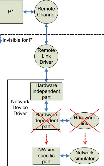
In order to interface the Remote Channels with the network simulator, a special ‘hardware specific’ implementation of a Network Device Driver is used. A Network Device Driver is a driver used to interface a Remote Channel with the communication hardware and is explained in detail in chapter 4. Special about this case is that the communication hardware is replaced by the network simulator. This special case is depicted in Figure 3-5, of which the original version can be found as Figure 4-3.
Remote Channel P1
Hardware link Invisible for P1
Remote Link Driver
Hardware independent
part
Hardware dependent
part Network
Device Driver
Network simulator NWsim
specific part
Figure 3-5 Network simulator interface
Packet representation
Chapter 3: Network Simulator 25
Node representation
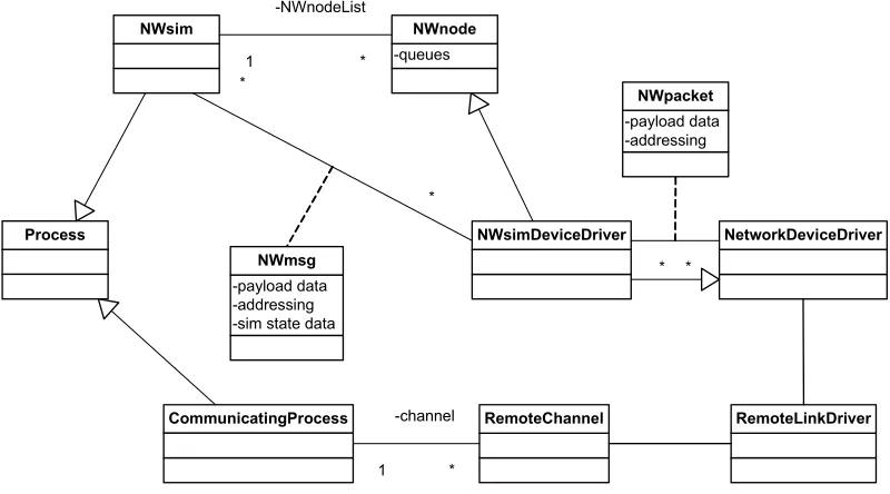
The network simulator uses objects of type NWnode to represent the nodes on the network. To connect the Remote Channel to the network, the NWsimDeviceDriver is inherited from the NWnode class (see the class diagram in Figure 3-6).
It might seem more logical to directly make the processor nodes (CommunicatingProcess in the figure) a network node, instead of indirectly via the network device driver. However, if each processor node would automatically be a network node, it would not be possible to have processor nodes that are not attached to any network, nor would it be possible to attach processor nodes to multiple networks. These scenarios are possible with the chosen class layout, because any process is allowed to have any number of NWimDeviceDrivers, including zero.
-queues
NWnode
NetworkDeviceDriver Process
NWsim
CommunicatingProcess
NWsimDeviceDriver
RemoteLinkDriver
-payload data -addressing
NWpacket
* * -payload data
-addressing -sim state data
NWmsg
*
*
RemoteChannel
1 -channel
* 1
-NWnodeList
*
Figure 3-6 Network simulator class diagram
3.3.4 Some minor changes for improved usability
A number of changes have been made to the original network simulator, in order to improve its usability.
Node numbering
The original TrueTime network simulator stores the information about the network nodes in an array. This constrains the numbering of the network nodes: the numbering must start at zero and no numbers may be skipped. While perfectly usable in the Simulink environment, these constraints cause some problems in the CTC++ simulation environment.
The main cause of these problems is that the network simulator objects and the a