scattering by defects and obstacles in layered media
Thesis by
Carlos A. P´erez Arancibia
In Partial Fulfillment of the Requirements for the Degree of
Doctor of Philosophy
California Institute of Technology Pasadena, California
2017
c
2017
Acknowledgements
First of all I would like to express my deepest gratitude for my advisor and mentor, Prof. Oscar Bruno, under whose caring, patient and generous guidance I could accomplish this thesis. His passion for mathematics and his assiduous pursuit of excellence and originality will always inspire me.
My sincerest thanks to Profs. Catalin Turc (NJIT) and Mark Lyon (U. of New Hampshire) who contributed to the development of the Windowed Green Function method, and Prof. Yue Ying Lau and Dr. Peng Zhang of the University of Michigan who proposed to us the interesting physics problems that eventually inspired the subject of this thesis.
I would also like to thank my thesis committee; Profs. Dan Meiron, Houman Owhadi and Peter Schroeder, for the useful comments and suggestions.
Thanks to my fellow groupmates and friends; Agust´ın Fernandez-Lado, Eldar Akhmet-galiyev, Emmanuel Garza-Gonzales, Thomas Anderson, Mart´ın Maas and Edwin Jimenez, for all the interesting discussions that took place over countless lunches and coffee breaks at Steele House. I would also like to thank Carmen Sirois and Sydney Garstang for their travel, scheduling and organizational support, and for making the office feel like home.
Special thanks to all the good friends I have made during my time at Caltech, specially Wael, Alex, Krishna, Cristi´an, Camila, George, Valentina, Soledad, Alejandro, Maricruz, Steven and Emma, with whom I shared so many great moments.
Last but not least, I would like to thank my family: my parents Osvaldo and Herminda, my brothers C´esar and N´estor and my aunt Rita, for their unconditional support.
My greatest gratitude goes to my beloved wife Ruby, who has selflessly accompanied me throughout this intellectual journey over all these years. This would not have been possible without your constant love and support for which I will be forever grateful.
Abstract
This thesis concerns development of efficient high-order boundary integral equation methods for the numerical solution of problems of acoustic and electromagnetic scattering in the presence of planar layered media in two and three spatial dimensions. The interest in such problems arises from application areas that benefit from accurate numerical modeling of the layered media scattering phenomena, such as electronics, near-field optics, plasmonics and photonics as well as communications, radar and remote sensing.
A number of efficient algorithms applicable to various problems in these areas are pre-sented in this thesis, including (i) A Sommerfeld integral based high-order integral equation method for problems of scattering by defects in presence of infinite ground and other layered media, (ii) Studies of resonances and near resonances and their impact on the absorptive properties of rough surfaces, and (iii) A novel Window Green Function Method (WGF) for problems of scattering by obstacles and defects in the presence of layered media. The WGF approach makes it possible to completely avoid use of expensive Sommerfeld integrals that are typically utilized in layer-media simulations. In fact, the methods and studies referred in points (i) and (ii) above motivated the development of the markedly more efficient WGF alternative.
Table of Contents
Acknowledgements iii
Abstract iv
1 Introduction 1
2 Scattering in planar layered media: Basic elements 8
2.1 Preliminary considerations . . . 9
2.2 Plane-wave scattering . . . 10
2.2.1 Maxwell’s equations in TE and TM polarizations . . . 10
2.2.2 Two-layer medium . . . 13
2.2.3 Multi-layer medium . . . 15
2.3 The Layer Green function . . . 16
2.3.1 Line source in a two-layer medium . . . 16
2.3.2 Point source in a two-layer medium . . . 23
2.3.3 Line and point sources in a three-layer medium . . . 26
2.3.4 Far-field pattern . . . 29
2.3.5 Numerical evaluation of the layer Green function . . . 46
2.4 Scattering by obstacles in a layered medium . . . 53
3 Layer Green function Method for problems of scattering by defects in layered media 62 3.1 Problem of scattering . . . 65
3.2 Integral equation formulations . . . 67
3.2.2 Problem Type II . . . 71
3.2.3 Problem Type III . . . 73
3.3 Nystr¨om method . . . 74
3.3.1 Discretization of integral equations . . . 74
3.3.2 Solution at resonant and near-resonant frequencies . . . 79
3.3.2.1 Task I: matrix-singularity detection . . . 80
3.3.2.2 Task II: analytic continuation . . . 81
3.4 Numerical examples . . . 84
3.5 Applications . . . 87
3.5.1 Electromagnetic power absorption due to bumps and trenches on flat surfaces . . . 88
3.5.2 Surface plasmon polariton scattering by defects in conducting surfaces 93 4 Windowed Green Function Method for layered media scattering 96 4.1 Preliminaries . . . 98
4.2 Windowed Green Function Method: Basic concepts . . . 101
4.2.1 Slow-rise windowing function . . . 101
4.2.2 Windowed integral equation: preliminary considerations . . . 103
4.2.3 Error sources in equation (4.2.2) . . . 105
4.2.4 Uniform super-algebraically fast convergence for all incidence angles . 107 4.2.5 Field evaluation: Near fields . . . 111
4.2.6 Field evaluation: Far fields . . . 113
4.3 Formal error analysis . . . 118
4.3.1 WGF solution of plane-wave-illuminated planar interface . . . 118
4.3.1.1 WGF error sources . . . 118
4.3.1.2 Error estimation for complex values of ξ . . . 122
4.3.2 Obstacle-free problem under plane-wave incidence: Numerical illustra-tions . . . 124
trations . . . 127
4.3.4 Formal error analysis via multiple-scattering . . . 130
4.4 Numerical Experiments . . . 134
5 Windowed Green Function Method for layered media scattering: Multiple layers 141 5.1 Preliminaries . . . 142
5.2 Integral representation . . . 146
5.3 Integral equation formulation . . . 152
5.4 Multilayer Windowed Green Function Method . . . 156
5.5 Field evaluation . . . 160
5.6 Alternative integral equation formulation . . . 163
5.7 Numerical examples . . . 168
6 Windowed Green Function Method for layered media scattering: Three dimensional case 177 6.1 Acoustics scattering . . . 177
6.1.1 Surface defect in a two-layer medium . . . 178
6.1.2 Two-layer waveguide . . . 182
6.1.3 Sound-hard obstacle in a two-layer medium . . . 183
6.1.4 Numerical examples . . . 186
6.2 Electromagnetic scattering . . . 192
7 Conclusions and future work 200 7.1 Conclusions . . . 200
7.2 Future work . . . 201
7.2.1 Accurate and efficient microstrip-antenna simulation . . . 202
7.2.2 Electromagnetic scattering by three-dimensional open surfaces . . . . 204
A Method of steepest descents 211
B.1 Exact solution . . . 213 B.2 Scattering poles . . . 214
C Dielectric half-plane under plane-wave illumination 215
D Existence and uniqueness 219
Chapter 1
Introduction
Early history. The interest on the propagation of light in presence of materials has re-mained at the forefront of human inquiry for over two millennia: the study of the phenomena of reflection, refraction and diffraction of electromagnetic waves dates back at least to the ancient Greeks [18]. Indeed, Greek philosophers and mathematicians were already familiar with certain aspects of the nature of light now encompassed within the theory of geomet-rical optics—such as the notion of rectilinear propagation, the law of reflection and the phenomenon of refraction. Yet the precise law of refraction was only established (experi-mentally) by Willebrord Snell in 1621.
Although successful at providing a good description of the reflection and refraction of light across (locally) planar material interfaces, the geometrical optics paradigm encountered severe difficulties at explaining the significantly more complex phenomenon of diffraction— which arises, for instance, as light impinges upon structures containing sharp boundaries (such as e.g. slits and screens). In fact, the so-called wave theory of light was originally put forth in an attempt to account for the diffraction phenomenon [34, 62]. In its early stages, however, this theory could not explain the reflection, refraction and rectilinear propagation of light. The first two aforementioned difficulties were overcame by Christian Huygens, who, relying on the famous principle that now bears his name1, was able to re-derive from
It took several decades until Augustin Fresnel in his celebrated “M´emoire sur la loi des modifications que la r´eflexion imprime a la lumi`ere polaris´ee”, published in 1819, demon-strated that diffraction can indeed be explained by applying Huygens’ principle and Young’s principle of interference. Remarkably, in that same memoir Fresnel provided the presently well-known expressions for the amplitude of the reflected and transmitted waves that arise when a plane-wave impinges on the flat interface between two homogeneous media with different optical properties. Fresnel’s memoire contains also the formula for the amplitudes of the multiple reflections that take place between the two parallel boundaries of a single homogeneous plate of finite-thickness and, furthermore, it describes how these results could be extended to account for more than one plate [124]. This formula has been re-derived independently by a number of authors, including George Stokes [120] and George Airy [2], the former of whom gave the complete solution to the problem of scattering of a plane-wave by a planar multilayered medium. Fresnel’s analysis of diffraction was later put on a firm mathematical basis by Gustav Kirchhoff, who around 1882 established an integral represen-tation formula which expresses a scalar-wave-field at an arbitrary point in terms of the field values and its normal derivative at an arbitrary closed surface. (This representation formula was derived earlier in acoustics for monochromatic time-harmonic waves by Helmholtz in 1859.) The corresponding integral representation formulae for (vectorial) electromagnetic fields were not available until 1939, when Stratton and Chu published their well known contribution [121].
In the meantime, the seemingly disconnected developments on electricity and magnetism were unified by James Clerk Maxwell. Maxwell’s works published between 1861 and 1862, which convey his celebrated system of differential equations, led him subsequently to conjec-ture that light waves are in fact electromagnetic waves. Maxwell’s conjecconjec-ture regarding the nature of light was empirically verified by Heinrich Hertz in 1888 [116]. As is well-known, Maxwell’s and Hertz’s discoveries turned out to have enormous practical consequences. Ap-plying Maxwell’s ideas pioneers experimentalists such as Marconi and Braun, who received the Nobel prize in 1909, started the era of wireless radio communications [115].
closely to the present dissertation—attracted considerable attention at the beginning of the 20th century in connection with theoretical efforts seeking to explain long-distance trans-mission of radio signals. Indeed, using a two-layer model that regards the earth and the air as homogeneous conducting and dielectric half-spaces, respectively, Jonathan Zenneck [138] studied the possibility that the earth surface could support a surface wave (also known as lateral wave) with low attenuation. Using this two-layer model Zenneck showed that a sur-face wave with the aforementioned characteristics (which additionally decays exponentially away from the planar interface) could exist, yet his work did not consider an excitation mechanism [131].
The excitation problem was studied mathematically by Arnold Sommerfeld [117], who obtained expressions for the fields produced by electric and magnetic dipoles located over the earth’s surface—under the assumptions inherent in Zenneck’s air/earth model. Sommer-feld’s solution is expressed in terms of certain Fourier-Bessel integrals known asSommerfeld integrals, which, unfortunately, cannot be evaluated in closed form. (A detailed discussion concerning Sommerfeld integrals can be found in the recent review [90] by Michalsky and Mosig.) Deforming the integration path from real-axis into the complex plane Sommerfeld identified two contributions—stemming from the branch cuts of the integrand and from the residue of a pole (the Sommerfeld pole), respectively. Sommerfeld’s 1909 paper [117] also contains an asymptotic analysis of the solution for large lateral distances which, famously, turned out to be erroneous. Sommerfeld’s results were eventually corrected and largely improved in various subsequent contributions, including very recent ones (see [90] and refer-ences therein). Further extensions of these ideas include studies of surface-waves arising in multi-layer models of the earth.
(PEC) scatterers. In 1907, for example, Lord Rayleigh [109] obtained a Fourier-Bessel series solution for the problem of scattering of a plane-electromagnetic wave by a single cylindrical bump with semi-circular cross-section on a PEC half-space. A year later, Mie [91] presented the exact solution for the problem of scattering of a plane-electromagnetic wave by a PEC sphere in free space. These ideas were later utilized to solve the closely related surface-defect problem for which of a PEC semi-spherical boss (or bump, in our nomenclature) is placed on a PEC half-space [126]. Unfortunately, however, separation-of-variables techniques could not effectively deal with penetrable layered media problems, as no series expansions are known to satisfy the suitable transmission conditions at the planar interfaces between two dielectric or finitely-conducting layers.
finally, BIE methods do not suffer from dispersion errors, which is a highly desirable property in the context of wave propagation problems.
To highlight these issues we mention the contribution [40], one of whose authors is also the author of the renowned FDTD text [122] (finite-difference time-domain). In particular, the contribution [40] utilizes the FDTD scheme to solve the problem of scattering of a plane electromagnetic wave by a two-dimensional circular dielectric scatterer. The wavelength of the incident plane wave in this example is 500 nm and the diameter of the circles is 5µm— which makes the circles 10 wavelengths in diameter. Using 100 points per wavelength the FDTD discretization required around 12 million grid points in the interior of each one of the circles to achieve errors of±15 percent of the value of the exact solution. The total number of grid points needed to achieve such errors was, of course, much larger than 12 million, as the FDTD scheme also required a fine discretization of the exterior domain including the PML regions, that must be placed at a certain distance from the obstacles to suppress unwanted features such as frequency-dependent reflections [122]. Comparable errors are obtained in this thesis for similar problems on the basis of discretizations containing a total of the order of 100 points. Thus, as is well known, use of integral equation methods enable solution of a wide range of problems that lie well outside the range of applicability of volumetric methods. In spite of these advantages, integral equation methods for problems of scattering in presence of layered media have remained inefficient—in view of the expense required for computation of the point values of the Green function suitable for layered media—which has typically rendered BIE treatment of large scale three-dimensional layered-media scattering problems essentially unfeasible. As discussed in what follows, this thesis provides an efficient integral-equation alternative for the solution of layered-media problems.
integrals, equals the (total field) solution of the problem of scattering of a point source embedded in one of the layers. Thus, a scattering solution produced by means of the LGF automatically enforces the transmission conditions on the planar interfaces.
In the earlier stages of this thesis work an improved and extended high-order LGF-based integral equation method [104] was introduced which can be used to tackle general problems of scattering by defects in the presence of layered media in two-dimensional space (Chapter 3). The proposed method enjoys several advantages: a) it requires evaluation of a minimal number of integral operators (and, thus, a minimal number of Sommerfeld-integrals); b) it is based on a highly-efficient procedure we introduced (on the basis of windowing methods) for evaluation of Sommerfeld integrals; and c) it incorporates a novel algorithm for resolution of spurious resonances that arise in our minimal integral-equation formulation.
The interest in the problems of scattering by obstacles and defects in layered media arose from a collaboration with a group of applied physicists at The University of Michigan seeking to quantify electromagnetic power absorption that arises as electromagnetic fields illuminate rough conducting surfaces [105]. This collaboration led to the development and validation of the LGF approach described above. In particular, numerical studies based on our LGF algorithm revealed that a connection exists between enhanced power absorption and the existence of certain “pseudo-resonant” frequencies—that correspond to scattering poles near the real axis—at which large currents are induced near the boundary of the defect; see Section 3.5.1. As discussed in that section, further, the LGF algorithm was also utilized to study pseudo-resonance phenomenon in the context of surface plasmons scattering by micro-cavities in metals.
method is fast, accurate, flexible and easy to implement. In particular straightforward modifications of existing (accelerated or unaccelerated) solvers suffice to incorporate the WGF capability. The mathematical basis of the method is simple: the approach relies on a certain integral equation that is smoothly windowed by means of a low-rise windowing function, and is thus supported on the union of the obstacle and a small flat section of the interface between the two penetrable media. Various numerical experiments presented in this thesis demonstrate that both the near- and far-field errors resulting from the proposed approach decrease faster than any negative power of the window size. In some of those examples the proposed method is up to thousands of times faster, for a given accuracy, than a corresponding LGF method (Figure 4.14). Analysis and generalizations of the WGF method to problems of scattering by obstacles in layered media composed by any finite number of layers in two (Chapter 5) and three spatial dimensions (Chapter 6) are also included in this dissertation.
Chapter 2
Scattering in planar layered media:
Basic elements
The present chapter concerns three classical problems of scattering by layered media, namely, 1) scattering of a plane-wave by a planar layered medium, 2) scattering of a point-source field by a planar layered medium and evaluation of associated Sommerfeld integrals, and 3) scat-tering of a plane-wave by an bounded obstacle embedded in a planar layered medium, under the simplifying assumption (that is eliminated in Chapter 3) that the obstacle boundary does not intersect any of the planar interfaces between the layers. In particular, this chap-ter summarizes certain well-known aspects of the aforementioned problems as well as novel results concerning the numerical evaluation of Sommerfeld integrals and their asymptotics (Sections 2.3.4 and 2.3.5, respectively).
few representative numerical examples.
2.1
Preliminary considerations
Throughout this thesis we consider planar layered media composed by N (N > 1) layers Dj = {−dj < y < −dj−1} of homogeneous dielectric/conducting materials. We let Πj =
{y=−dj}denote the plane at the interface between the layersDj andDj+1, j = 1, . . . , N−1,
(see Figure 2.1), where dj+1 > dj and d0 =−∞ and dN =∞.
Π1
Π2
ΠN−2
ΠN−1
D1
D2
DN−1
...
DN
...
z
x y
Figure 2.1: Planar layered medium.
Under the assumption that the electromagnetic field is driven by a time-harmonic source with time dependence given by e−iωt (whereω >0 denotes the angular frequency), it follows
that the total electric and total magnetic fieldsE andHsatisfy Maxwell’s equations [18, 64]
curlE−iωµjH = 0, (2.1a)
curlH+iωεjE = 0, (2.1b)
within the layer Dj, j = 1, . . . , N, with material constants µj and εj = ε0j + iσj
ω . Here ε0j,
σj ≥ 0 and µj > 0 denote the electrical permittivity, the electrical conductivity, and the
magnetic permeability of the medium Dj, respectively.
value of the electric (resp. magnetic) field at Πj from the subdomain Dj, these continuity
conditions can be expressed in the forms
n×[Ej−Ej+1] = 0, (2.2a)
n×[Hj −Hj+1] = 0, (2.2b)
on Πj, where n denotes the unit normal vector which points from the dielectric medium
Dj+1 to the dielectric medium Dj.
The transmission conditions (2.2) become boundary conditions when one of the media, say Dj+1, is made of a infinitely conducting material. In fact, modeling Dj+1 as a perfect
electric conductor (PEC), that is, setting σj+1 = ∞, the transmission conditions (2.2a)
and (2.2b) reduce to the boundary condition
n×Ej =0 (2.3)
at the PEC boundary.
2.2
Plane-wave scattering
2.2.1
Maxwell’s equations in TE and TM polarizations
The present section describes how, under certain symmetry assumptions, the Maxwell’s system (2.1) in three-dimensional space can be equivalently expressed as a decoupled system of Helmholtz equations in a (two-dimensional) plane.
Consider an electromagnetic field (E,H), solution of (2.1), which remains constant along the z-axis:
E(r) = Ex(x, y)ex+Ey(x, y)ey +Ez(x, y)ez,
H(r) = Hx(x, y)ex+Hy(x, y)ey+Hz(x, y)ez,
easy to check that the field (E,H) is a solution of Maxwell’s equations (2.1) if and only if the equations
∂Ez
∂y −iωµjHx = 0, (2.4a)
−∂Ez
∂x −iωµjHy = 0, (2.4b)
∂Ey
∂x − ∂Ex
∂y
−iωµjHz = 0, (2.4c)
and
∂Hz
∂y +iωεjEx = 0, (2.5a)
−∂Hz
∂x +iωεjEy = 0, (2.5b)
∂Hy
∂x − ∂Hx
∂y
+iωεjEz = 0, (2.5c)
are satisfied. It follows from (2.4) and (2.5) that the electromagnetic field is completely determined by Ez and Hz:
E = i
ωε ∂Hz
∂y ex− i ωε
∂Hz
∂x ey+Ezez, (2.6a)
H = − i
ωµ ∂Ez
∂y ex+ i ωµ
∂Ez
∂x ey +Hzez. (2.6b)
Substituting these expressions into (2.4c) and (2.5c), and defining the wavenumber kj by
kj2 =ω2εjµj =ω2
ε0j+ iσj ω
µj, (2.7)
we obtain the Helmholtz equations ∂2E
z
∂x2 +
∂2E
z
∂y2 +k 2
jEz = 0, (2.8a)
∂2H
z
∂x2 +
∂2H
z
∂y2 +k 2
for the z components Ez and Hz. It is easy to check that equations (2.6) and (2.8) are
equivalent to (2.4) and (2.5).
The electromagnetic field (E,H) obtained by solving (2.8a) for Ez, assuming Hz = 0, is
known as the transverse electric (TE) field, while the solution obtained by solving (2.8b) for Hz, assuming Ez = 0, is known as the transverse magnetic (TM) field.
Noting, on the other hand, that at the interface Πj the z-coordinates of the tangential
components of the fields are given by
(n×Ej)·ez = −
i ωεj∇
Hjz·n =−
i ωεj
∂Hjz
∂n ,
(n×Hj)·ez =
i ωµj∇
Ejz·n=
i ωµj
∂Ejz
∂n ,
it follows that the transmission conditions (2.2) can be expressed (in terms of Ez and Hz
only) as
Ejz =Ej+1,z,
∂Ejz
∂n =ν
E j
∂Ej+1,z
∂n , (2.9a)
Hjz =Hj+1,z,
∂Hjz
∂n =ν
H j
∂Hj+1,z
∂n , (2.9b)
at the interface Πj, where
νjE = µj µj+1
and νjH = εj εj+1
. (2.10)
Similarly, the boundary condition (2.3) at the boundary of a PEC leads to the following boundary conditions for the transverse components of the electric and magnetic fields:
Ez = 0, (2.11a)
∂Hz
2.2.2
Two-layer medium
Consider a layered medium composed of two half-spaces D1 = {y >0} and D2 = {y <0}
characterized by their respective wavenumbers, k1 andk2, and let Π1 ={y= 0}be the
inter-face between the half-spaces. Further, let an incident electromagnetic plane-wave (Einc,Hinc)
of the form
Einc = (p×k) eik·r and Hinc = 1 ωµ1
k×Einc, (2.12)
be given, wherep= (px, py, pz) is a constant vector parallel toH, and where, without loss of
generality, a wavevector of the formk= (k1x,−k1y,0),k1y ≥0, with|k|=
q
k2
1x+k12y =k1is
assumed. Clearly, thez-independent plane-wave (2.12), which is determined by its transverse components Einc
z =E0ei(k1xx−k1yy) (E0 =−pyk1x−pxk1y) and Hzinc =H0ei(k1xx−k1yy) (H0 =
k1pz), is a solution of (2.1) in D1.
Similarly, the total electromagnetic field (Ej,Hj) in Dj, which equals the incident plus
the reflected field inD1, and equals the transmitted field inD2, is completely determined by
Ejz and Hjz, which satisfy homogeneous Helmholtz equations (2.8a) and (2.8b) in Dj with
k =kj and transmission conditions (2.9a) and (2.9b) withj = 1.
Applying the method of separations of variables and using the continuity of total trans-verse fields across Π1, we get that the physically meaningful solutions Ez and Hz of (2.8a)
and (2.8b) respectively, are given by
Ez(x, y) = E0eik1xx
e−ik1yy+RTE
12 eik1yy in D1,
TTE
12 e−ik2yy in D2,
(2.13a)
and
Hz(x, y) =H0eik1xx
e−ik1yy+RTM
12 eik1yy in D1,
TTM
12 e−ik2yy in D2,
(2.13b)
where k2y =
p
k2
2 −k21x with the complex square root defined such that Imk2y ≥ 0 and
Rek2y > 0. Note, in particular, that k2y equals
p
k2
2−k21x if k22 ≥ k21x, and it equals
ipk2
condi-tions (2.9a) and (2.9b), we obtain the following systems of equacondi-tions:
1 +RTE12 =T12TE, k1y(1−R12TE) = k2yν1ET12TE,
1 +RTM12 =T12TM, k1y(1−RTM12 ) =k2yν1HT12TM,
whose solutions are the Fresnel coefficients [18]:
RTEj,j+1 = kjy−ν
E j kj+1,y
kjy+νjEkj+1,y
, Tj,jTE+1 = 2kjy kjy+νjEkj+1,y
, (2.14a)
RTMj,j+1 = kjy−ν
H j kj+1,y
kjy+νjHkj+1,y
, Tj,jTM+1 = 2kjy kjy+νjHkj+1,y
. (2.14b)
The fields E0RTE12 eik1xx+ik1yy and H0RTM12 eik1xx+ik1yy in (2.13) are referred to as reflected
fields, while the fields E0T12TEeik1xx−ik2yy and H0T12TMeik1xx−ik2yy are referred to as
transmit-ted fields. The physical interpretation of the reflectransmit-ted fields and the transmittransmit-ted fields in the case Imk2 = 0, k22 ≥k21x, corresponds to plane-waves that propagate upwards and
down-wards, respectively, whose directions of propagation are determined by Snells’s law [18]. The transmitted fields corresponding to wavenumbersk2
2 < k21x or Imk2 >0, in turn, correspond
to evanescent waves that decay exponentially towards the lower half-plane, and thus they do not propagate.
Finally, we note that in the presence of a PEC half-planeD2, the total transverse electric
and magnetic fields are given by
Ez(x, y) =E0eik1xx
e−ik1yy−eik1yy in D 1,
0 in D2,
(2.15a)
and
Hz(x, y) = H0eik1xx
e−ik1yy+ eik1yy in D 1,
0 in D2,
(2.15b)
in TE and TM polarizations respectively.
considered.
2.2.3
Multi-layer medium
Utilizing the physical nomenclature considered in Section 2.2.2 we now derive the solution of the problem of scattering of a plane electromagnetic wave by a layered medium composed by N layers, with planar interfaces Πj determined by positive numbersdj,j = 1, . . . , N−1. The
derivations presented in this subsection are based on the waves-tracing arguments presented in [41], which date back to the seminal work of G. G. Stokes [120]. Similar derivations can also be found [20, 124].
For the sake of brevity in the exposition only the TE-polarization case in presented in this section. The TM-polarization case is completely analogous. Letting kjy =
q
k2
j −k12y,
j = 2, . . . , N, where once again the complex square root is defined such that Imkjz ≥0 and
Rekjy >0, the total transverse electric field is expressed as
Ez(x, y) =E0eik1xx
e−ik1yy+ReTE
12 eik1y(y+2d1) in D1,
ATE
j
n
e−ikjyy+ReTE
j,j+1eikjy(y+2dj) o
in Dj, 2≤j ≤N,
(2.16)
in terms of the generalized reflection coefficients ReTE
j,j+1 and amplitudes ATEj . Clearly Ez
in (2.16) satisfies the Helmholtz equation with wavenumber kj in each one of the layers Dj,
j = 1, . . . , N.
In order to determine the unknown coefficientsReTE
j,j+1 andATEj , we observe that the
down-going wave within Dj, which equals ATEj eikjydj−1 at Πj−1, is given by the transmitted wave
from the layer above, which equals TTE
j−1,jATEj−1eikj−1,ydj−1 at Πj−1, plus the reflected wave by
the layer below that is reflected by the layer above, which equalsRTE
j,j−1ATEj ReTEj,j+1eikjy(2dj−dj−1)
at Πj−1. Therefore, it follows from (2.16) that the down-going wave at Πj−1 satisfies
ATEj eikjydj−1 =TTE
j−1,jATEj−1eikj−1,ydj−1+RTEj,j−1ATEj Rej,jTE+1eikjy(2dj−dj−1). (2.17)
On the other hand, the up-going wave within Dj−1, which equals ATEj−1RejTE−1,jeikj−1,ydj−1
which equals ATE
j−1RjTE−1,jeikj−1,ydj−1 at Πj−1, plus the transmission of the up-going wave in
layer below, which equalsTTE
j,j−1ATEj ReTEj,j+1eikjy(2dj−dj−1) at Πj−1. Thus, from (2.16) we obtain
that the up-going wave at Πj−1 satisfies
ATEj−1ReTEj−1,jeikj−1,ydj−1 =ATE
j−1RTEj−1,jeikj−1,ydj−1+Tj,j−1ATEj ReTEj,j+1eikjy(2dj−dj−1). (2.18)
From Equations (2.17) and (2.18) we then obtain the following recursive relations for the amplitudes and generalized reflection coefficients:
ATEj = T
TE
j−1,jATEj−1ei(kj−1,y−kjy)dj−1
1−RTE
j,j−1ReTEj,j+1e2ikjy(dj−dj−1)
, (2.19a)
e
RTEj−1,j = RTEj−1,j+T
TE
j,j−1ReTEj,j+1TjTE−1,je2ikjy(dj−dj−1)
1−RTE
j,j−1ReTEj,j+1e2ikjy(dj−dj−1)
, (2.19b)
where RTE
j and TjTE are defined in (2.14a).
The condition that there is no up-going wave in the lowermost layer, i.e., ReTE
N,N+1 = 0,
allows us to find the generalized reflection coefficients ReTE
j,j+1, j = 1, . . . N −1, recursively.
Having obtained the generalized reflection coefficients, the amplitude coefficients ATE
j , j =
2, . . . , N are determined from (2.19a) using the condition that ATE 1 = 1.
2.3
The Layer Green function
2.3.1
Line source in a two-layer medium
In this section we consider the problem of evaluation of the electromagnetic field produced by a line source along a straight line parallel to the planar interface contained in a two-layer medium. In view of the discussion in Section 2.2.1 above, this is a two-dimensional problem. Thus, it can be equivalently formulated as the problem of computing the Green function for the Helmholtz equation in a layered medium composed by the half-planes D1 ={y > 0}= R2+ and D2 = {y < 0} = R2−, with wavenumbers k1 and k2, respectively, whose common
The desired Green function, G(·,r0) :R2 →C, satisfies
∆rG(r,r0) +kj2G(r,r0) = −δr0 in Dj, j = 1,2, G(r,r0)y=0+ = G(r,r0)
y=0− on Π1, ∂G
∂y(r,r
0)
y=0+
= ν∂G ∂y(r,r
0)
y=0−
on Π1,
(2.20a)
and the Sommerfeld radiation condition [45] at infinity:
lim
|r|→∞
p |r|
∂G ∂|r|(r,r
0)−ik
jG(r,r0)
= 0 uniformly in all directions r
|r| ∈Dj,
(2.20b) where the constant ν equals νE
1 in TE-polarization and ν1H in TM-polarization (see
defini-tion (2.10)), and where δr0 ∈ S0(R2) denotes the Dirac delta distribution supported at the point r0 ∈ R2. Throughout this section, we refer to r0 = (x0, y0) as the “source point”, and
tor = (x, y) as the “observation point”.
As is known, Gcan be computed explicitly in terms of Fourier integrals [20], sometimes called Sommerfeld integrals. To obtain such explicit expressions, given a fixed pointr0 ∈Di,
i = 1,2, we define the functions gj(i)(r) = G(r,r0), r ∈ Dj, j = 1,2. Expressing gj(i) as
inverse Fourier transforms
gj(i)(x, y) = 1 2π
Z ∞
−∞b
gj(i)(ξ, y) eiξ(x−x0) dξ (2.21)
r0 ∈D1, the ODE system is given by
∂2bg(1) 1
∂y2 −γ 2 1bg
(1)
1 = −δy0 if y >0, ∂2bg(1)
2
∂y2 −γ 2 2bg
(1)
2 = 0 if y <0, b
g(1)1 (ξ,0) = bg2(1)(ξ,0), ∂bg(1)1
∂y (ξ,0) = ν ∂bg(1)2
∂y (ξ,0), whose unique physically admissible solution is
b
g1(1)(ξ, y) = e
−γ1|y−y0| 2γ1
+R12
e−γ1|y+y0| 2γ1
(y >0),
b
g2(1)(ξ, y) = T12
eγ2y−γ1y0
2γ1
(y <0),
(2.22)
where
R12=
γ1−νγ2
γ1+νγ2
, T12=
2γ1
γ1+νγ2
, (2.23)
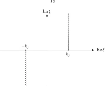
and γj = γj(ξ) =
q
ξ2−k2
j. The determination of physically admissible branches of the
functions γj(ξ) =
p
ξ−kj
p
ξ+kj require selection of branch cuts for each one of the two
associated square root functions. The relevant branches, which are determined by consider-ation of Sommerfeld’s radiconsider-ation condition, are−3π/2≤arg(ξ−kj)< π/2 for
p
ξ−kj and
−π/2 ≤ arg(ξ+kj) < 3π/2 for
p
ξ+kj. In particular, for real values of ξ and a positive
real wavenumberkj, we have thatγj(ξ) =
q
ξ2−k2
j ≥0 if |ξ| ≥kj andγj(ξ) = −i
q
k2
j −ξ2
if |ξ| < kj with
q
k2
j −ξ2 > 0. The domain of definition of the function γj is depicted in
Reξ Imξ
kj
−kj
Figure 2.2: Branch-cuts and domain of definition for the function γj =
q
ξ2−k2
j.
Similarly, the ODE system for r0 ∈D2 is given by
∂2bg(2) 1
∂y2 −γ 2 1bg
(2)
1 = 0 if y >0,
∂2bg2(2)
∂y2 −γ 2 2bg
(2)
2 = −δy0 if y <0,
b
g(2)1 (ξ,0) = bg2(2)(ξ,0), ∂bg(2)1
∂y (ξ,0) = ν ∂bg(2)2
∂y (ξ,0), whose solution can be expressed as
b
g1(2)(ξ, y) = T21
e−γ1y+γ2y0
2γ2
(y >0),
b
g2(2)(ξ, y) = e−
γ2|y−y0
|
2γ2
+R21
e−γ2|y+y0
|
2γ2
(y <0),
(2.24)
where
R21=
νγ2−γ1
νγ2+γ1
, T21=
2νγ2
νγ2+γ1
. (2.25)
the well-known expression of the free-space Green function [41, 134] i
4H
(1)
0 (kj|r −r0|) =
1 4π
Z ∞
−∞
e−γj|y−y0|
γj
eiξ(x−x0) dξ, (2.26)
we obtain the following form of the Green function
G(r,r0) =
i 4H (1)
0 (k1|r−r0|) +
1 4π
Z ∞
−∞
R12
e−γ1|y+y0
|
γ1
eiξ(x−x0) dξ, y0, y >0,
1 4π
Z ∞
−∞
T12
eγ2y−γ1y0
γ1
eiξ(x−x0) dξ, y0 >0, y <0,
1 4π
Z ∞
−∞
T21
e−γ1y+γ2y0
γ2
eiξ(x−x0) dξ, y0 <0, y >0, i
4H
(1)
0 (k2|r−r0|) +
1 4π
Z ∞
−∞
R21
e−γ2|y+y0| γ2
eiξ(x−x0) dξ, y0, y <0,
(2.27)
where R12 =R12(ξ) and T12 =T12(ξ) (resp. R21 = R21(ξ) and T21 = T21(ξ)) are defined in
(2.23) (resp. (2.25)).
The fact that the expression in (2.27) satisfies the Sommerfeld radiation condition (2.20b) is shown in Section 2.3.4 below.
Remark 2.3.1. It is easy to see from (2.27) and the definition ofR12, T12, R21 andT21 that
the layer-Green function G(·,r0), solution of (2.20), satisfies
G(r,r0) =
G(r0,r), y, y0 >0, νG(r0,r), y > 0, y0 <0,
1 νG(r
0,r), y <0, y0 >0,
G(r0,r), y, y0 <0.
(2.28)
Thus, taking the limits as y0 →0± in (2.28) we obtain
G(r,r0)y0=0+ =G(r0,r)
y0=0+ =G(r0,r)
y0=0− = 1 νG(r,r
0)
y0=0−, ∂G
∂y0(r,r0)
y0=0+
= ∂G ∂y0(r0,r)
y0=0+
= ν∂G ∂y0(r0,r)
y0=0−
= ∂G ∂y0(r,r0)
y0=0− ,
for an observation point r = (x, y) ∈ D1 (y > 0), where the identities G(r0,r)
y0=0+ =
G(r0,r)y0=0− and ∂G∂y0(r0,r)
y0=0+ =ν∂G∂y0(r0,r)
y0=0− follow from the transmission conditions in (2.20a). Similarly, for an observation point r = (x, y)∈D2 (y <0) we obtain
G(r,r0)y0=0+ =
1 νG(r
0,r)
y0=0+ =
1 νG(r
0,r)
y0=0− = 1 νG(r,r
0)
y0=0−, ∂G
∂y0(r,r 0)
y0=0+
= 1 ν
∂G ∂y0(r
0,r)
y0=0+
= ∂G ∂y0(r
0,r)
y0=0−
= ∂G ∂y0(r,r
0)
y0=0− .
(2.30)
Therefore we conclude that the function G(r,·) :R2 →C satisfies
∆r0G(r,r0) +k2
jG(r,r0) = −δr in Dj, j = 1,2,
νG(r,r0)y0=0+ = G(r,r0)
y0=0− on Π1, ∂G
∂y0(r,r 0)
y0=0+
= ∂G
∂y0(r,r 0)
y0=0−
on Π1,
and the radiation condition
lim
|r|→∞
p |r0|
∂G
∂|r0|(r,r0)−ikjG(r,r0)
= 0 uniformly in all directions r
0
|r0| ∈Dj.
(2.31) In order to improve the rate of decay as |ξ| → ∞ of the functions that define bgj(i)(ξ, y), so that the spatial derivatives of G can be computed differentiating under the integral sign of the inverse Fourier transform even in the case y=y0 = 0, we express (2.22) and (2.24) as
b
g1(1)(ξ, y) =
e−γ1|y−y0
|
2γ1
+
1−ν 1 +ν
e−γ1|y+y0
|
2γ1
+ ν(k
2
2−k12) e−γ1(y+y
0)
(1 +ν)(γ1+νγ2)(γ1+γ2)γ1
(y >0),
b
g2(1)(ξ, y) =
1 1 +ν
e−γ1(y0−y)
γ1
+
eγ2y−γ1y0
γ1+νγ2 −
1 1 +ν
e−γ1(y0−y)
γ1
(y <0),
for r0 ∈D1, and
b
g1(2)(ξ, y) =
ν 1 +ν
e−γ2|y−y0
|
γ2
+
νe−γ1y+γ2y0
γ1+νγ2 −
ν 1 +ν
e−γ2(y−y0)
γ2
(y >0),
b
g2(2)(ξ, y) = e−
γ2|y−y0
|
2γ2
+
ν−1 ν+ 1
e−γ2|y+y0
|
2γ2
+ ν(k
2
1−k22) eγ2(y+y
0)
(1 +ν)(γ1+νγ2)(γ2+γ1)γ2
(y <0), (2.32b) for r0 ∈D2.
Note that the following asymptotic estimates hold for the last term in each of the formu-lae (2.32) above:
e
−γ1(y+y0)
(γ1+νγ2)(γ1+γ2)γ1
=O(e−|ξ|(y+y
0)
|ξ|−3), (y, y0 >0),
e
γ2y−γ1y0
γ1+νγ2 −
1 1 +ν
e−γ1(y0−y)
γ1
=O(e−|ξ|(y
0
−y)
|ξ|−3), (y <0, y0 >0),
νe
−γ1y+γ2y0
γ1+νγ2 −
ν 1 +ν
e−γ2(y−y0)
γ2
=O(e−|ξ|(y−y
0)
|ξ|−3), (y >0, y0 <0),
ν(k
2
1−k22) eγ2(y+y
0)
(1 +ν)(γ1+νγ2)(γ2+γ1)γ2
=O(e−|ξ||y
0+y
||ξ|−3), (y, y0 <0),
(2.33)
as |ξ| → ∞. Thus, taking the inverse Fourier transform (2.21) of bgj(i) in (2.32) using the identity in (2.26) we arrive to
G(r,r0) =
i 4H (1)
0 (k1|r−r0|) +
i 4
1−ν 1 +ν
H0(1)(k1|r−r0|) + Φ(1)R (r,r0), y, y0 >0,
i 2
1 1 +ν
H0(1)(k1|r−r0|) + ΦT(1)(r,r0), y <0, y0 >0, i
2
ν 1 +ν
H0(1)(k2|r−r0|) + ΦT(2)(r,r0), y >0, y0 <0, i
4H
(1)
0 (k2|r−r0|) +
i 4
ν−1 ν+ 1
H0(1)(k2|r−r0|) + Φ(2)R (r,r0), y, y0 <0,
(2.34a) where r0 = (x0,−y0) denotes the image of the source point r0 = (x0, y0) with respect to the
Φ(Ti),i= 1,2, are explicitly given by
Φ(1)R (r,r0) = ν(k
2 2 −k21)
π(1 +ν)
Z ∞
0
e−γ1(y+y0)cos(ξ(x−x0))
γ1(γ1+γ2)(γ1+νγ2)
dξ,
Φ(1)T (r,r0) = 1 π
Z ∞
0
eγ2y−γ1y0
γ1+νγ2 −
eγ1(y−y0)
(1 +ν)γ1
cos(ξ(x−x0)) dξ,
Φ(2)T (r,r0) = ν π
Z ∞
0
e−γ1y+γ2y0
γ1+νγ2 −
e−γ2(y−y0)
(ν+ 1)γ2
cos(ξ(x−x0)) dξ,
Φ(2)R (r,r0) = ν(k
2 1 −k22)
π(ν+ 1)
Z ∞
0
eγ2(y+y0)cos(ξ(x−x0))
γ2(γ2+γ1)(γ1+νγ2)
dξ.
(2.34b)
The expressions in (2.34) are utilized in Section 2.3.5 to numerically evaluate the layer Green function.
In view of the enhanced decay (2.33) of each one of the integrands in (2.34b) together with the Lebesgue’s dominated convergence theorem, the gradient of the Green function (2.34a) can be evaluated from the expressions above by differentiation under the integral sign.
2.3.2
Point source in a two-layer medium
In this section we consider the full three-dimensional problem of finding the layer Green function for the Helmholtz equation in a two-layer medium. Lettingδr0 ∈ S0(R3) denote the Dirac delta function supported at the source point r0 = (x0, y0, z0) ∈ R3, we have that the
sought Green function, G(·,r0) :R3 →C, satisfies
∆rG(r,r0) +kj2G(r,r0) = −δr0 in Dj, j = 1,2, G(r,r0)|y=0+ = G(r,r0)|y=0− on Π1,
∂G ∂z (r,r
0)
y=0+
= ν ∂G ∂z(r,r
0)
y=0−
on Π1,
as well as the Sommerfeld radiation condition [45] at infinity
lim
|r|→∞|r|
∂G ∂|r|(r,r
0)−ik
jG(r,r0)
= 0 uniformly in all directions r
|r| ∈Dj ⊂R
3.
(2.35b)
As in the two-dimensional case, G can be computed explicitly by means of the Fourier transform. To obtain such explicit expression, given a fixed point source point r0 ∈ Di we
define the function gj(i)(r) =G(r,r0) for an observation point r ∈ Dj, and we express it as
the inverse two-dimensional Fourier transform
g(ji)(x, y, z) = 1 (2π)2
Z ∞
−∞
Z ∞
−∞b
gj(i)(ξ1, ξ2, y) ei(ξ1(x−x
0)+ξ
2(z−z0)) dξ
1dξ2. (2.36)
Taking advantage of the cylindrical symmetry of the problem, we make the following change of variables:
x−x0 =ρcosα, z−z0 =ρsinα,
for the spatial variables, where ρ=p(x−x0)2 + (y−y0)2 and 0≤α≤2π, and
ξ1 =ξcosβ, ξ2 =ξsinβ, (2.37)
for the spectral variables, whereξ =pξ2
1 +ξ22 and 0≤β ≤2π.
Note that since gj(i)(x, y, z) is axisymmetric, i.e., does not depend on the angle θ, its Fourier transform bgj(i)(ξ1, ξ2, y) does not depend on α. Therefore, we can simply write b
gj(i)(ξ1, ξ2, y) = bgj(i)(ξ, y). Then, using the change of variables (2.37) and the integral
repre-sentation of the Bessel function [134]
J0(t) =
1 2π
Z 2π
0
eitcosβ dβ,
we obtain that (2.36) can be equivalently expressed as a Hankel transform
g(ji)(x, y, z) = 1 2π
Z ∞
0 b
Replacing (2.38) in the partial differential equation (2.35a), we obtain the same system of ODEs for bg(ji)(ξ, y) obtained in the previous section, whose solution is given in (2.22) for
r0 ∈D1, and in (2.24) for r0 ∈D2.
Subsequently, taking the inverse Hankel transform as defined in (2.38), of bgj(i)(ξ, y) and using the identity
eikj|r−r0|
4π|r−r0| =
1 4π
Z ∞
0
e−γj|y−y0|
γj
J0(ξρ)ξdξ, (2.39)
we obtain that the Green function is given by
G(r,r0) =
eik1|r−r0|
4π|r−r0| +
1 4π
Z ∞
0
R12
e−γ1|y+y0
|
γ1
J0(ξρ)ξdξ, y, y0 >0,
1 4π
Z ∞
0
T12
eγ2y−γ1y0
γ1
J0(ξρ)ξdξ, y <0, y0 >0,
1 4π
Z ∞
0
T21
e−γ1y+γ2y0
γ2
J0(ξρ)ξdξ, y >0, y0 <0,
eik2|r−r0|
4π|r−r0| +
1 4π
Z ∞
0
R21
e−γ2|y+y0
|
γ2
J0(ξρ)ξdξ, y, y0 <0,
(2.40)
where R12 =R12(ξ) and T12 =T12(ξ) (resp. R21 = R21(ξ) and T21 = T21(ξ)) are defined in
(2.23) (resp. (2.25)).
As in the two-dimensional case, the Green function can be equivalently expressed as
G(r,r0) =
eik1|r−r0|
4π|r−r0| +
1−ν 1 +ν
eik1|r−r0|
4π|r−r0| + Φ
(1)
R (r,r0), y, y0 >0,
1 1 +ν
eik1|r−r0|
2π|r−r0| + Φ
(1)
T (r,r0), y <0, y0 >0,
ν 1 +ν
eik2|r−r0| 2π|r−r0| + Φ
(2)
T (r,r0), y >0, y0 <0,
eik2|r−r0|
4π|r−r0| +
ν−1 ν+ 1
eik1|r−r0| 4π|r−r0| + Φ
(2)
R (r,r0), y, y0 <0,
(2.41a)
the plane Π1 ={y= 0}and where the functions Φ(Ri) and Φ
(i)
T , i= 1,2, are given by
Φ(1)R (r,r0) = ν(k
2 2 −k21)
2π(1 +ν)
Z ∞
0
e−γ1(y+y0)
γ1(γ1+γ2)(γ1+νγ2)
J0(ξρ)ξdξ,
Φ(1)T (r,r0) = 1 2π
Z ∞
0
eγ2y−γ1y0
γ1+νγ2 −
eγ1(y−y0)
(1 +ν)γ1
J0(ξρ)ξdξ,
Φ(2)T (r,r0) = ν 2π
Z ∞
0
e−γ1y+γ2y0
γ1+νγ2 −
e−γ2(y−y0)
(ν+ 1)γ2
J0(ξρ)ξdξ,
Φ(2)R (r,r0) = ν(k
2 1 −k22)
2π(ν+ 1)
Z ∞
0
eγ2(y+y0)
γ2(γ2+γ1)(γ1+νγ2)
J0(ξρ)ξdξ.
(2.41b)
In view of the asymptotic expansion for the Bessel functionJ0(z) as|z| → ∞[76, 134], the
integrands in (2.41b) above decay more slowly than their two-dimensional counterparts (2.33) as |ξ| → ∞. However, they and their gradients with respect to r and r0 are still absolutely integrable for all source and observation points.
2.3.3
Line and point sources in a three-layer medium
This section deals with the problem of computation of the Green function for a three-layer medium in two and three dimensional spaces. Both Green functions are given by the solution of the transmission problem:
∆rG(r,r0) +k2jG(r,r0) = −δr0 in Dj, j = 1,2, G(r,r0)y=
−d+1 = G(r,r0)
y=−d−1 on Π1,
G(r,r0)y=−d+
2 = G(
r,r0)y=−d−
2 on Π2,
∂G ∂y(r,r
0)
y=−d+1
= ν1
∂G ∂y(r,r
0)
y=−d−1
on Π1,
∂G ∂y(r,r
0)
y=−d+2
= ν2
∂G ∂y(r,r
0)
y=−d−2
on Π2,
(2.42)
at infinity follows from the far-field form of the physically correct solution G obtained by Fourier transformations techniques.
As in the previous sections, we start by expressing G as an inverse Fourier trans-form (2.21) in the two-dimensional case, and as an inverse Hankel transtrans-form (2.38) in the three-dimensional case. Replacing the resulting expressions forGin (2.42) and applying the corresponding inverse transform we then obtain a system of ODEs for G =G(r,r0) in the spectral form, which is denoted by bg(ji)(ξ, y) for observation and source points r ∈ Dj and
r0 ∈ Di, respectively. Solving the ODE system, eliminating all the exponentially growing
solutions (as |ξ| → ∞) and enforcing the transmission conditions at the planar interfaces Π1
and Π2, the functionsbg(ji)(ξ, y),i, j = 1,2,3 are obtained in closed form. In detail, we obtain
that for a source point r0 ∈D1, the solution of the ODE system is given by
b
g(1)1 (ξ, y) = 1 2γ1
e−γ1|y−y0|+ R12+R23e
2γ2(d1−d2)
1 +R12R23e2γ2(d1−d2)
e−γ1(y+y0+2d1)
,
b
g(1)2 (ξ, y) = 1 2γ1
T12ed1(γ2−γ1)
[1 +R12R23e2γ2(d1−d2)] n
eγ2y−γ1y0+R
23e−γ2(y+2d2)−γ1y
0o
,
b
g(1)3 (ξ, y) = 1 2γ1
T23T12ed1(γ2−γ1)+d2(γ3−γ2)
[1 +R12R23e2γ2(d1−d2)]
eγ3y−γ1y0,
(2.43a)
where
Rij =
γi−νiγj
γi+νiγj
if j > i, νiγj −γi
νiγj +γi
if i > j,
and Tij = 1 +Rij.
The square root branches in the definition ofγ3 = p
ξ2−k2 3 =
√
ξ−k3 √
ξ+k3 are the same
that were previously utilized in the definition of the functionsγj,j = 1,2. For a point source
in the middle layer r0 ∈D2, on the other hand, we obtain
b
g1(2)(ξ, y) = 1 2γ2
T21
1 +R23e−2γ2(d2+y
0)
eγ2y0
[1−R21R23e2γ2(d1−d2)]
e−d1(γ1−γ2)e−γ1y,
b
g2(2)(ξ, y) = 1 2γ2
n
e−γ2|y−y0|+Aeγ2(y−y0)+Be−γ2(y−y0)
o
,
b
g3(2)(ξ, y) = 1 2γ2
T23
1 +R21e2γ2(d1+y
0)
[1−R21R23e2γ2(d1−d2)]
ed2(γ3−γ2)eγ3y−γ2y0,
where
A= R21[1 +R23e−
2γ2(d2+y0)] e2γ2(d1+y0)
1−R21R23e2γ2(d1−d2)
and B = R23[1 +R21e
2γ2(d1+y0)] e−2γ2(d2+y0)
1−R21R23e2γ2(d1−d2)
.
Finally, for a point source r0 ∈D3, we have
b
g1(3)(y;ξ) = 1 2γ3
T21T32ed1(γ2−γ1)+d2(γ3−γ2)
[1 +R32R21e2γ2(d1−d2)]
eγ3y0−γ1y,
b
g2(3)(y;ξ) = 1 2γ3
T32ed2(γ3−γ2)
[1 +R32R21e2γ2(d1−d2)] n
e−γ2y+γ3y0+R
21eγ2(y+2d1)+γ3y
0o
,
b
g3(3)(y;ξ) =
1 2γ3
e−γ3|y−y0|+ R32+R21e
2γ2(d1−d2)
1 +R32R21e2γ2(d1−d2)
eγ3(y+y0+2d2)
.
(2.43c)
The layer Green function G is then obtained by evaluating the corresponding inverse integral transform ((2.21) in the two-dimensional case and (2.38) in the three-dimensional case) of the expressions in (2.43). Note that the point source term is explicitly obtained in both cases utilizing the identities (2.26) and (2.39) in the two- and three-dimensional cases respectively.
In order to improve the decay of the integrands in the resulting integral representation of G, the functions bg(ji), i, j = 1,2,3, are expressed as hbg(ji)−egj(i)i+egj(i), where egj(i) denotes the leading order asymptotic expansion of bgj(i) as |ξ| → ∞, which is obtained utilizing the relations
Rij =
1−νi
1 +νi
+ 2νi(k
2
j −ki2)
(1 +νi)(γi+νiγj)(γi+γj)
= 1−νi 1 +νi
+O(|ξ|−2) (j > i),
Tij =
2 1 +νi
+ 2νi(k
2
j −ki2)
(1 +νi)(γi+νiγj)(γi+γj)
= 2
1 +νi
+O(|ξ|−2) (j > i), e−γjy = e−γiy1 +O(|ξ|−1)
(2.44)
follows by taking inverse transform of hbg(ji)−egj(i)i+eg(ji) for i, j = 1,2,3.
2.3.4
Far-field pattern
The present section is devoted to the asymptotic analysis of the two- and three-dimensional two-layer Green function (which were obtained in Sections 2.3.1 and 2.3.2), as |r| → ∞, for a given point source r0 in space and fixed wavenumbers k1 and k2 (k1 > 0 and Imk2 ≥ 0).
The analysis presented here is based on the method of steepest descent for which we refer to [15, 20, 21, 41, 51]. The relevant steepest-descents formulae are summarized in Appendix A. Some of the results obtained in this subsection follow directly from the analysis provided by Bleistein [15, Section 8.1] for the asymptotic approximation of layer Green function in the limit when k1 → ∞ for fixed spatial variables and a fixed index of refractionn =k2/k1.
In detail, this section provides the leading order asymptotic expansion of the reflected and transmitted wave fields produced by point sources at r0 ∈ Dj, j = 1,2, respectively,
at an observation point r ∈ D1 (y > 0) where |r| 1. The leading order asymptotic
expansions for the transmitted and reflected fields produced by point sources at r0 ∈ Dj,
j = 1,2, respectively, at an observation point r ∈ D2 (y < 0), |r| 1, can be obtained
following a completely analogous procedure.
Polar coordinates. Expressing both the observation and source points in polar coordi-nates (r = |r|(cosθ,sinθ), θ ∈ [0, π], r0 = |r0|(cosθ0,sinθ0) for θ0 ∈ [0,2π]), the relevant
reflected and transmitted fields in (2.27) for the presenty >0 case become
GR(r,r0) =
1 4π
Z ∞
−∞
R12
e−|r0|(iξcosθ0+γ
1sinθ0)
γ1
e|r|(iξcosθ−γ1sinθ) dξ r0 ∈D
1 =R2+
, (2.45a)
and
GT(r,r0) =
1 4π
Z ∞
−∞
T21
e−|r0|(iξcosθ0
−γ2sinθ0)
γ2
e|r|(iξcosθ−γ1sinθ) dξ r0 ∈D
respectively. For notational simplicity we introduce the change of variablesξ =k1ζ; we thus
obtain
GR(r,r0) =
1 4π
Z ∞
−∞
gR(ζ) e|r|φ(ζ) dζ, (2.46a)
GT(r,r0) =
ν 2π
Z ∞
−∞
gT(ζ) e|r|φ(ζ) dζ, (2.46b)
where
gR(ζ) =
p
ζ2−1−νpζ2−n2 p
ζ2−1 +νpζ2−n2
e−i|r0|k1(ζcosθ0−i√ζ2−1 sinθ0)
p
ζ2−1 , (2.47a)
gT(ζ) =
e−ik1|r0|(ζcosθ0+i
√
ζ2−n2sinθ0)
p
ζ2−1 +νpζ2−n2 , (2.47b)
φ(ζ) = ik1(ζcosθ+i p
ζ2−1 sinθ), (2.47c)
and pζ2−1 = γ
1(ζk1)/k1 and p
ζ2−n2 =γ
2(ζk1)/k1.
Saddle points. In view of (2.47c) it follows that the first two derivatives of the phase function φ are given by
φ0(ζ) = ik1 cosθ+i
ζsinθ
p
ζ2−1 !
and φ00(ζ) = k1sinθ (ζ2−1)pζ2−1.
From the saddle-point conditionφ0(ζ
0) = 0 we see that there is only one saddle point, given
byζ0 = cosθ ∈R, at which
φ(ζ0) =ik1 and φ00(ζ0) = −
ik1
sin2θ.
With reference to equation (A.2) it therefore follows that the directions of steepest descent at the saddle point are given byαp =−α/2+(2p+1)π/2,p= 0,1, whereα = argφ00(ζ0) = −π/2
(here we select argz ∈(−π, π]). Clearly, α0 = 3π/4 and α1 =−π/4.
In oder to asymptotically determine the path of steepest descent passing through ζ0 we
Consequently, the phase function satisfies
φ(ζ) = k1ζ(−sinθ+icosθ) +O(|ζ|−1)
= −k1{sinθReζ+ cosθImζ}+ik1{cosθReζ−sinθImζ}+O(|ζ|−1).
Since on the path of steepest descent, which is denoted byD, the imaginary part ofφremains constant and equal to k1, we conclude that D approaches the line
Imζ = cosθ
sinθ Reζ− 1
sinθ as |ζ| → ∞,
for Reζ >0. For large values of |ζ|, with ζ in the second or third quadrants, on the other hand, we have pζ2 −1 ∼ −ζ. Thus, in this case we obtain that the steepest descent path
approaches the line
Imζ =−cosθ
sinθ Reζ+ 1
sinθ as |ζ| → ∞, for Reζ <0.
This analysis implies that D intersects the real axis at two points; at the saddle point ζ = cosθ, of course, and at ζ = 1/cosθ, where the latter was obtained by noting that
φ
1 cosθ
=−k1
sin2θ
|cosθ| +ik1.
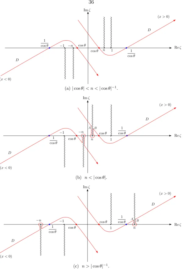
The paths of steepest descent for the cases x >0 and x <0, are depicted in Figure 2.3. From (A.2) it follows directly that, provided gT and gR are continuous and do not vanish
at the point ζ =ζ0, the saddle point contribution to the asymptotic expansion of (2.46a) as |r| → ∞ is given by
G(1)R (r,r0) = i 4π
sinθ−iν√cos2θ−n2
sinθ+iν√cos2θ−n2 s
2π k1|r|
e−i|r0|k1cos(θ+θ0)eik1|r|−iπ/4, (2.48a)
given by
G(1)T (r,r0) = iν 2π
sinθe−ik1|r0|(cosθcosθ0+i√cos2θ−n2sinθ0) sinθ+iν√cos2θ−n2
s
2π k1|r|e
ik1|r|−iπ/4. (2.48b)
There are, however, four potential saddle points which are concurrently branch points at which this assumption is certainly not true. These are ζ0 =±n and ζ0 =±1.
In the case of a saddle point given by ζ0 = ±n it can be shown that the integrands gR
and gT can be expressed as p(ζ) +q(ζ)(ζ −ζ0)1/2, where p and q are analytic functions in
a neighborhood of ζ0. Thus, from (A.3) we readily check that formulae (2.48) still remain
valid in this case.
A saddle point given by ζ0 = cosθ = ±1, on the other hand, presents an additional
difficulty, as the phase function ceases to be analytic at those points. Nevertheless, formulae (2.48) remain valid for θ = 0, π for as a long as θ0 6= 0, π. This can be proved by applying
the steepest descents method to obtain the leading order terms of the expansions of GR
as |r − r0| → ∞ and GT as |r − r0| → ∞ first, and subsequently using the fact that
|r−p|=|r| − r·p
|r| +O
1
|r|
as |r| → ∞, where p=r0 in the case of GR and p=r0 in the
case of GT.
Polar singularities. We next consider the possibility of contributions to the asymptotic expansions of GR and GT due to poles of the functions gR and gT, respectively, which could
arise when such poles happen to lie inside the region bounded by the ζ-real-axis to the path of steepest descent D. From (2.47) it follows that the possible poles of gT and gR must be
given by the solutions of the algebraic equation
(ζ2−1)−ν2(ζ2−n2) = 0. (2.49)
Clearly, solutions to this equation exist only when ν 6=±1 and are given by
ζ =± r
n2ν2−1
Thus, in view of (2.50), in the case of a real wavenumberk2 the solutions of (2.49) are either
real or imaginary.
Assume for the time being that both poles are real. In order for the denominator
p
ζ2−1 +νpζ2−n2 = [γ
1(ζk1) +νγ2(ζk1)]/k1 to vanish, both γ1(ζk1) and γ2(ζk1) have to
be either purely real or purely imaginary. If both are real, we have, by the definition of the functions γj, j = 1,2, that γj(ζk1)≥ 0. Therefore, they can not cancel each other. If both
are imaginary, in turn, we have that Imγj(ζk1) ≤ 0, and thus, again, they can not cancel
each other. Therefore, the functions gT and gR do not have poles on the real axis.
Let us now consider the possibility of imaginary poles. By the definition ofγj,j = 1,2,we
can easily check that−3π/4≤argγj(±itk1)≤ −π/4,t >0, which means that both complex
numbers γj(±itk1),j = 1,2,lie on the same half-plane in the complex plane. Therefore, we
conclude that gR and gT do not have pole singularities in the complex plane when k2 ∈R.
We now consider the possibility of pole singularities ofgRandgT for a complex
wavenum-ber k2 ∈ C, Imk2 > 0 in TM polarization in the case of a non-magnetic medium, i.e.,
µ1 =µ2 =µ0. (Since ν = 1 in TE polarization, there are no poles ofgT andgRin this case).
Note that we are allowing the permittivity of the lower half-plane to be such that Reε2 <0,
which, as matter of fact, corresponds to feasible physical values for highly conducting metals at low frequency [83].
Under the aforementioned assumptions we have thatν =ε1/ε2 = 1/εr and n2 =k22/k21 =
ε2/ε1 = 1/ν =εr, whereεr =ε2/ε1 =|εr|eiα,α ∈(0, π). Replacing these identities in (2.50)
we obtain that the solutions of (2.49) are given by ζ =±ζp, where
ζp =
r
1 ν+ 1 =
r
ε2
ε1+ε2
=
r
εr
εr+ 1
.
Since 1 +εr =|1 +εr|eiβ, β ∈(0, α), we obtain
ζp =
r
εr
1 +εr
=
s |εr|
|1 +εr|
ei(α−β)/2,
order for ζp to be a pole of gR and gT then, we need the condition γ1(ζpk1) +νγ2(ζpk2) = 0
to be satisfied. Under the present definition of the functions γj, j = 1,2 we have
γ1(ζpk1) = k1 q
ζ2
p −1 =
ik1
ζp
√ε
r
if εr ∈R+1,
−ik1
ζp
√ε
r
if εr ∈R−1,
(2.51)
and
γ2(ζpk1) = k1 q
ζ2
p −εr =
ik1ζp√εr if εr∈R+2, −ik1ζp√εr if εr∈R−2,
(2.52)
where the connected regions R±j are such that R+j ∩Rj−=∅,R+j ∪R−j ={z ∈C: Imz >0},
j = 1,2.
Thus, in order for ζp to be a pole of gR and gT, it is necessary that ζp ∈ R+1 ∩R2− or
ζp ∈R−1 ∩R+2. Clearly, such conditions lead to
γ1(ζpk1) +νγ2(ζpk1) = ik1
ζp
√ε
r −
ik1
εr
ζp√εr = 0.
As is well-documented [90, 131], the poles±ζp of the layer Green function in spectral form,
which are known in the literature as Sommerfeld poles, depend on definition of γj, j = 1,2.
When present, a Sommerfeld pole may give rise to a surface-wave of the form uζp(r) =
ceik1ζp|x|−ik1ζp/√εry in the asymptotic expansion ofG
R andGT. In order for this surface-wave
to be physically meaningful, it is necessary that ζp ∈R1+; otherwise uζp does not satisfy the
radiation condition. This surface-wave has historically received various names (Zeneck wave, surface plasmon polariton, Brewster mode, or Fano mode) depending on the values of the real and imaginary parts of εr [90]. In any case, it is clear that uζp decays exponentially
fast as |r| = px2+y2 → ∞, in virtue of the fact that Imζ
p > 0 and Im (ζp/√εr) < 0.
Branch points. In order to assess the asymptotic contribution of the branch points to the overall value of the integrals in (2.46), we distinguish three cases: Case (a): |cosθ|<Ren <
|cosθ|−1, Case (b): Ren < |cosθ|, and Case (c): Ren > |cosθ|−1. The integration paths
for each of these case are shown in Figure 2.3.
It is clear that Case (a) leads to no additional contributions from the branch points, as the path of steepest descent D does not cross the branch cuts stemming from the branch points at ζ =±n.
In Cases (b) and (c), in turn, the steepest descent path may or may not cross the branch cut starting at the branch point ζ = n (resp. ζ = −n) when cosθ > 0 (resp. cosθ < 0), depending on how large Imn is. When it does, D has to be locally deformed around the branch cut, as it is shown in Figure 2.3b and 2.3c. The new path encompasses two new critical points, A and B