Distributed Control and Optimization for Communication and Power Systems

(1)

Distributed Control and Optimization for Communication

and Power Systems

Thesis by

Qiuyu Peng

In Partial Fulfillment of the Requirements for the Degree of

Doctor of Philosophy

California Institute of Technology Pasadena, California

2016

(2)

c

2016

(3)

This thesis is dedicated to

my girlfriend Huan,

whose love made this possible,

and my parents,

(4)

Acknowledgements

First and foremost, I would like to express my deepest gratitude to my advisor, Professor Steven Low, for his continuous support of my Ph.D study. Steven is a great scholar who dedicates to work on impactful and hard research problems. He introduced me to a variety of research areas in both communication and power networks. He gave me freedom and supported me to work on projects based on my own interests. It is his enthusiasm on research that motivates me to think big and work on important research problems no matter how hard they look. I could not have imagined having a better advisor and mentor for my Ph.D study.

Besides my advisor, I would like to thank the rest of my thesis committee: Professor John Doyle, Professor Mani Chandy, Professor P. P. Vaidyanathan and Professor Adam Wierman. It’s really my great honor to have them on my committee. They gave me their insightful comments and encouragement. I learned advanced control theory in John’s class. Mani raised many interesting questions in both my candidacy exam and thesis defense that were very beneficial in the completion of my thesis. I was in P. P. V’s class on signal processing and he could always explain the complex formula from different perspectives. Adam gave me great help and advice on writing good papers and making presentations. He taught me how to communicate complicated ideas through plain English that people could easily understand.

I am also thankful to my former research advisor, Professor Xinbing Wang, for his guidance during my undergraduate study at Shanghai Jiao Tong University. I was a junior when I joined Xinbing’s lab. He gave me much advice on doing research and encouraged me to pursue my Ph.D. in US. It was his advice and encouragement that made it possible for me to study at Caltech.

My collaborators also gave me their great supports: Anwar Walid, Jaehyun Hwang from Bell Lab, Minghua Chen from Chinese University of Hong Kong and Seungil You, Yujie Tang from Caltech. It was a great pleasure to work with these great minds and I am grateful for all of those fruitful discussions.

I am grateful to all the colleagues in my research group RSRG. Special thanks to an incomplete list of current and past group members: Minghong Lin, Zhenhua Liu, Lingwen Gan, Desmond Cai, Changhong Zhao, Xiaoqi Ren and Niangjun Chen, etc.

(5)

and cozy environment. It is a paradise for studying and doing research. I want to thank the great help from staff members, especially Christine Ortega, Sydney Garstang and Tanya Owen.

(6)

Abstract

We are at the cusp of a historic transformation of both communication system and electricity system. This creates challenges as well as opportunities for the study of networked systems. Problems of these systems typically involve a huge number of end points that require intelligent coordination in a distributed manner. In this thesis, we develop models, theories, and scalable distributed optimization and control algorithms to overcome these challenges.

This thesis focuses on two specific areas: multi-path TCP (Transmission Control Protocol) and

electricity distribution system operation and control. Multi-path TCP (MP-TCP) is a TCP exten-sion that allows a single data stream to be split across multiple paths. MP-TCP has the potential to greatly improve reliability as well as efficiency of communication devices. We propose a fluid model for a large class of MP-TCP algorithms and identify design criteria that guarantee the existence, uniqueness, and stability of system equilibrium. We clarify how algorithm parameters impact TCP-friendliness, responsiveness, and window oscillation and demonstrate an inevitable tradeoff among these properties. We discuss the implications of these properties on the behavior of existing algo-rithms and motivate a new algorithmBalia (balanced linked adaptation) which generalizes existing algorithms and strikes a good balance among TCP-friendliness, responsiveness, and window oscilla-tion. We have implementedBalia in the Linux kernel. We use our prototype to compare the new proposed algorithmBalia with existing MP-TCP algorithms.

Our second focus is on designing computationally efficient algorithms for electricity distribution system operation and control. First, we develop efficient algorithms for feeder reconfiguration in distribution networks. The feeder reconfiguration problem chooses the on/off status of the switches in a distribution network in order to minimize a certain cost such as power loss. It is a mixed integer nonlinear program and hence hard to solve. We propose a heuristic algorithm that is based on the recently developed convex relaxation of the optimal power flow problem. The algorithm is efficient and can successfully computes an optimal configuration on all networks that we have tested. Moreover we prove that the algorithm solves the feeder reconfiguration problem optimally under certain conditions. We also propose a more efficient algorithm and it incurs a loss in optimality of less than 3% on the test networks.

(7)

(8)

List of Figures

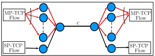
2.1 Test network for the definition of TCP friendliness. The link in the middle is the only

bottleneck link with capacityc. . . 15

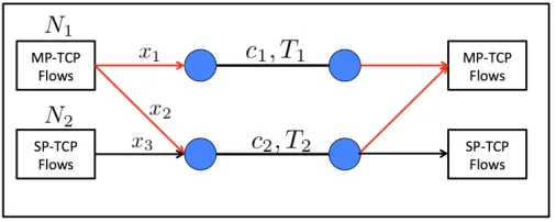
2.2 Network for our Linux-based experiments on TCP friendliness and responsiveness, with N1MP-TCP flows and N2single-path TCP flows sharing two links of capacity,c1,c2, and propagation delay (single trip) T1, T2. MP-TCP flows maintain two routes with ratex1,x2. Single-path TCP flows maintain one route with rate x3. . . 21

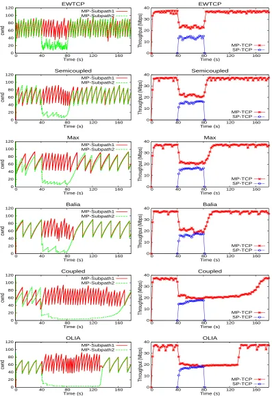
2.3 Responsiveness Performance: congestion window trajectory of MP-TCP for each path (left column). TCP starts at time 40s and ends at 80s. The throughput of SP-TCP and total throughput of MP-SP-TCP are shown in the right column. Parameters: T1=T2= 10ms,c1=c2= 20Mbps, andN1= 1, N2= 5. . . 22

2.4 Window oscillation: the red trajectories represent throughput fluctuations experienced by the application in the case of MP-TCP and the case of single-path TCP. . . 24

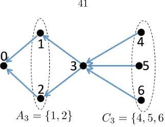
3.1 Notations of graph G(N,E), where the ancestor and children set of node 3 are also labeled explictly. . . 41

3.1 Notations for Balanced Network. . . 42

3.1 Notations for Unbalanced Networks. . . 46

4.1 Possible network topology with one redundant line. . . 54

4.2 A line Network . . . 56

4.3 Intuitions of Algoirthm 4.1. . . 58

4.1 A modified SCE 47-bus feeder. The blue bar (1) represents the substation bus, the red dots (13, 17, 19, 23, 24) represent buses with PV panels, and the other dots represent load buses without PV panels. . . 63

4.2 A modified SCE 56-bus feeder. The blue bars (1, 57, 58) represent the substation buses and the red dot (45) represents the bus with PV panels. . . 65

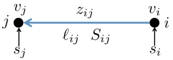
5.1 Message passing for a nodei. . . 88

(13)

6.1 Simulation results for 2065 bus distribution network. . . 102 6.2 Topologies for tree and fat tree networks. . . 104

(14)

List of Tables

2.1 MP-TCP algorithms . . . 11

2.2 How design choices affect MP-TCP performance. . . 20

2.3 TCP friendliness (same RTTs): Average throughput (Mbps) and 95% confidence in-terval of MP-TCP and single-path TCP users. (T1 =T2 = 5ms, c1 =c2 = 60Mbps andN1=N2= 30) . . . 23

2.4 Basic behavior (WiFi/3G): throughput (Mbps) of a MP-TCP user and 95% confidence interval. (T1= 10ms,T2= 100ms,c1= 8Mbps,c2= 2Mbps,N1= 1, N2= 0) . . . 23

2.5 Responsiveness: convergence time (s) of MP-TCP and total throughput (Mbps) of all single-path TCP users. (T1=T2= 10ms,c1=c2= 20Mbps,N1= 1, N2= 5) . . . 24

4.1 Network of Fig. 4.1: Line impedances, peak spot load KVA, Capacitors and PV gen-eration’s nameplate ratings. . . 62

4.2 Summary on Brazil-135 Bus System . . . 63

4.3 Summary on Tai-83 Bus System . . . 64

4.4 Network of Fig. 4.2: Line impedances, peak spot load KVA, Capacitors and PV gen-eration’s nameplate ratings. . . 64

6.1 Multipliers associated with constraints(6.6g) . . . 99

6.1 Statistics of different networks . . . 103

6.2 Statistics of line and fat tree networks . . . 104

7.1 Multipliers associated with constraints (7.8g)-(7.8h) . . . 118

7.1 Statistics of different networks . . . 123

(15)

List of Algorithms

4.1 Network with one redundant line . . . 55

4.2 Network with one redundant line (simplified) . . . 56

4.3 General Network Reconfiguration . . . 61

4.4 General Network Reconfiguration (simplified) . . . 61

6.1 Initialization of the Algorithm . . . 101

6.2 Distributed OPF algorithm on Balanced Radial Networks . . . 102

7.1 Initialization of the Algorithm . . . 122

(16)

Chapter 1

Introduction

We are at the cusp of a historic transformation of both communication system and electricity system. This creates challenges as well as opportunities for the study of networked systems. Problems of these systems typically involve a huge number of end points that require intelligent coordinations in a distributed manner. In this thesis, we develop models, theories, and scalable distributed optimization and control algorithms that overcome these challenges.

Specifically, this thesis focuses on three topics: multi-path TCP,feeder reconfiguration in distri-bution systems anddistributed OPF algorithm on radial distribution networks.

1.1

Multipath TCP

Traditional TCP uses a single path through the network even though multiple paths are usually available in today’s communication infrastructure; e.g., most smart phones are enabled with both cellular and WiFi access, and servers in data centers are connected to multiple routers. Multi-path TCP (MP-TCP) has the potential to greatly improve application performance by using multiple paths transparently. It is being standardized by the MP-TCP Working Group of the Internet Engineering Task Force (IETF) [30]. We present a fluid model of MP-TCP and study how protocol parameters affect structural properties such as the existence, uniqueness and stability of equilibrium, the tradeoffs among TCP friendliness, responsiveness and window oscillation. These properties motivate a new algorithm that generalizes existing MP-TCP algorithms.

(17)

reasonably friendly to single-path TCP users. Recently, opportunistic linked increase algorithm (OLIA) is proposed as a variant of Coupled algorithm that is as friendly as the Coupled algorithm but more responsive [50]. See [77] for more references to early work on multi-path congestion control. Our goal is to develop structural understanding of MP-TCP algorithms so that we can system-atically trade off different properties such as TCP friendliness, responsiveness, and window oscilla-tion. Window oscillation can be detrimental to applications that require a steady throughput. For single-path TCP, one can associate a strictly concave utility function with each source so that the congestion control algorithm implicitly solves a network utility maximization problem [47, 62, 77]. The convexity of this underlying utility maximization guarantees the existence, uniqueness, and stability of most single-path TCP algorithms. For many MP-TCP proposals considered by IETF, it will be shown that the utility maximization interpretation fails to hold in general, necessitating the need for a different approach to understanding the equilibrium properties of these algorithms. Moreover the relations among different performance metrics, such as fairness, responsiveness, and window oscillation, need to be clarified.

We propose a fluid model for a large class of MP-TCP algorithms and the existence, uniqueness, and stability of system equilibrium are identified. The impact of algorithm parameters on TCP-friendliness, responsiveness, and window oscillation are clarified and an inevitable tradeoff among these properties are also derived. The implications of these properties on the behavior of exist-ing algorithms motivate the algorithm Balia, which outperforms all the existexist-ing algorithms in our experiment.

1.2

Feeder Reconfiguration in Distribution Networks

A primary distribution system consists of buses, distribution lines, and (sectionalizing and tie) switches that can be opened or closed. There are two types of buses. Substation buses (or just

substations) are connected to a transmission network from which they receive bulk power, andload buses that receive power from the substation buses. During normal operation the switches are configured so that

1. There is no loop in the network.

2. Each load bus is connected to a single substation.

(18)

The OFR problem is a combinatorial (on/off status of switches) optimization problem with nonlinear constraints (power flow equations) and can generally be NP-hard. Various algorithms have been developed to solve the OFR problems. Following the convention in [45], they roughly fall into two categories: formal methods and heuristic methods.

Formal methods solve the OFR problem using generic mixed integer optimization approaches. They usually require a significant amount of computation time, e.g. simulated annealing [17], ordinal optimization [24], bender decomposition [51], etc..

Heuristic methods exploit problem structures to solve OFR. They are usually more efficient than formal methods but lack theoretical guarantee on performance, e.g., iterative branch exchange approach [6, 19, 36] and successive branch reduction approach [35, 39, 65] etc..

We propose a new heuristic method with guaranteed performance. The effectiveness of this new approach is illustrated both through simulations on standard test systems and mathematical analysis. Specifically, the proposed algorithm only involves solving a small number of OPF problems andno

computationally intensive mixed-integer optimization. We prove that the proposed heuristic can obtain the global optimal solution under certain assumptions. Indeed global optimal configurations can always be found on the four practical networks in our simulations.

1.3

Distributed OPF Algorithm on Radial Distribution

Net-works

The optimal power flow (OPF) problem seeks to optimize certain objectives such as power loss and generation cost subject to power flow physics and operational constraints. It is a fundamental problem because it underlies many power system operations and planning problems such as economic dispatch, unit commitment, state estimation, stability and reliability assessment, volt/var control, demand response, etc. The continued growth of highly volatile renewable sources on distribution systems calls for real-time feedback control. Solving the OPF problems in such an environment has at least two challenges.

First, the OPF problem is hard to solve because of its nonconvex feasible set. Recently a new approach through convex relaxation has been developed. Specifically semidefinite program (SDP) relaxation [4] and second order cone program (SOCP) relaxation [44] have been proposed in the bus injection model, and SOCP relaxation has been proposed in the branch flow model [25, 27]. See the tutorial [60, 61] for further pointers to the literature. When an optimal solution of the original OPF problem can be recovered from any optimal solution of a convex relaxation, we say the relaxation is

(19)

many practical networks. In those cases we can rely on off-the-shelf convex optimization solvers to obtain a globally optimal solution for the nonconvex OPF problem.

Second, most algorithms proposed in the literature are centralized and meant for applications in today’s energy management systems that, e.g., centrally schedule a relatively small number of generators. In future networks that simultaneously optimize (possibly in real time) the operation of a large number of intelligent endpoints, a centralized approach will not scale because of its computation and communication overhead.

We will address the second challenge. Specifically, we develop computationally efficient dis-tributed algorithms that can scale to large real networks for both balanced and unbalanced radial distribution networks.

1.4

Thesis Overview

The thesis is organized as follows:

1. In Chapter 2, we develop a general theoretical framework to model mutli-path TCP, which leads to a better algorithm (Balia) that strikes a better balance among competing performance criteria. We also implementBalia in the Linux kernel. This work is based on [74, 75].

2. In Chapter 3, we formulate the optimal power flow problem on both balanced and unbal-anced networks and show how to solve them through second order cone program (SOCP) and semidefinite program (SDP) relaxation. They are the foundations of our works on feeder reconfiguration and distributed OPF algorithm.

3. In Chapter 4, we formulate the feeder reconfiguration problem in distribution networks, which is a mixed integer nonlinear program. We then develop heuristic algorithms and show the performance through both rigorous analysis and simulations on standard test networks. This work is based on [72, 73].

4. In Chapter 5, we first review alternating direction method of multipliers(ADMM). Based on the general ADMM, we propose efficient centralized and distributed algorithms for a broad class of graphical optimization problems.

(20)

Chapter 2

Multipath TCP: Analysis, Design

and Implementation

Multi-path TCP (MP-TCP) has the potential to greatly improve application performance by using multiple paths transparently. A fluid model is proposed for a large class of MP-TCP algorithms and the existence, uniqueness, and stability of system equilibrium are identified. The impact of algorithm parameters on TCP-friendliness, responsiveness, and window oscillation are clarified and an inevitable tradeoff among these properties are also derived. The implications of these properties on the behavior of existing algorithms are discussed and they motivate the algorithmBalia(balanced linked adaptation), which generalizes existing algorithms and strikes a good balance among TCP-friendliness, responsiveness, and window oscillation. Balia is implemented in the Linux kernel and compared with existing MP-TCP algorithms.

Literature Traditional TCP uses a single path through the network even though multiple paths are usually available in today’s communication infrastructure; e.g., most smart phones are enabled with both cellular and WiFi access, and servers in data centers are connected to multiple routers. Multi-path TCP (MP-TCP) has the potential to greatly improve application performance by using multiple paths transparently. It is being standardized by the MP-TCP Working Group of the Internet Engineering Task Force (IETF) [30]. In this chapter we present a fluid model of MP-TCP and study how protocol parameters affect structural properties such as the existence, uniqueness and stability of equilibrium, the tradeoffs among TCP friendliness, responsiveness, and window oscillation. These properties motivate a new algorithm that generalizes existing MP-TCP algorithms.

(21)

can respond slowly in a dynamic network environment. A different algorithm is proposed in [89] (which we refer to as the Max algorithm) which is more responsive than the Coupled algorithm and still reasonably friendly to single-path TCP users. Recently, opportunistic linked increase algorithm (OLIA) is proposed as a variant of Coupled algorithm that is as friendly as the Coupled algorithm but more responsive [50]. See [77] for more references to early work on multi-path congestion control. Our goal is to develop structural understanding of MP-TCP algorithms so that we can system-atically tradeoff different properties such as TCP friendliness, responsiveness, and window oscilla-tion. Window oscillation can be detrimental to applications that require a steady throughput. For single-path TCP, one can associate a strictly concave utility function with each source so that the congestion control algorithm implicitly solves a network utility maximization problem [47, 62, 77]. The convexity of this underlying utility maximization guarantees the existence, uniqueness, and stability of most single-path TCP algorithms. For many MP-TCP proposals considered by IETF, it will be shown that the utility maximization interpretation fails to hold in general, necessitating the need for a different approach to understanding the equilibrium properties of these algorithms. Moreover the relations among different performance metrics, such as fairness, responsiveness, and window oscillation, need to be clarified.

Summary The main contributions of this work are three-fold. First we present a fluid model that covers a broad class of MP-TCP algorithms and identify the exact property that allows an algorithm to have an underlying utility function. This implies that some MP-TCP algorithms, e.g., the Max algorithm [89], has no associated utility function. We prove conditions on protocol parameters that guarantee the existence and uniqueness of the equilibrium, and its asymptotical stability. Indeed, algorithms that fail to satisfy these conditions, e.g. the Coupled algorithm, can be unstable and can have multiple equilibria as shown in [89]. Second, we clarify how protocol parameters impact TCP friendliness, responsiveness, and window oscillation and demonstrate the inevitable tradeoff among these properties. Finally, based on our understanding of the design space, we proposeBalia (Balanced linked adaptation) MP-TCP algorithm that generalizes existing algorithms and strikes a good balance among these properties. This algorithm has been implemented in the Linux kernel and we evaluate its performance using our Linux prototype.

We now summarize our proposedBalia MP-TCP algorithm. Each sourceshas a set of routesr. Each route rmaintains a congestion window wr and measures its round-trip time τr. The window adaptation is as follows:

• For each ACK on route r∈s,

wr←wr+

xr

τr(Pxk)2

_{1 +}_α

r 2

4 +αr 5

(22)

• For each packet loss on router∈s,

wr←wr−

wr

2 min{αr,1.5}, (2.2)

wherexr:=wr/τrandαr:=max_x{xk}

r .

2.1

Multipath TCP model

In this section we first propose a fluid model of MP-TCP and then use it to model MP-TCP algorithms in the literature. Unless otherwise specified, a boldface letterx∈ Rn denotes a vector

with components xi. We use x−i := (x1, . . . , xi−1, xi+1, . . . , xn) to denote the n−1 dimensional vector withoutxi andkxkk:= (Pxki)1/k to denote theLk-norm ofx. Given two vectorsx,y∈Rn, x≥ymeansxi≥yi for all componentsi. A capital letter denotes a matrix or a set, depending on the context. A symmetric matrixP is said to bepositive (negative) semidefinite ifxT_P_x_≥₀₍_≤₀₎ for any x, and positive (negative) definite if xT_P_x _> ₀₍_< _{0) for any} _x ₆₌ ₀_{. For any matrix} _P_, define [P]+ := (P+PT)/2 to be its symmetric part. Given two arbitrary matricesA and B (not necessarily symmetric), AB means [A−B]+ is positive semidefinite. For a vectorx,diag{x} is a diagonal matrix with entries given byx.

2.1.1

Fluid model

Consider a network that consists of a set L = {1, . . . ,|L|} of links with finite capacities cl. The network is shared by a setS ={1, . . . ,|S|}of sources. Available to sources∈Sis a fixed collection of routes (or paths) r. A route r consists of a set of links l. We abuse notation and use s both to denote a source and the set of routesr available to it, depending on the context. Likewise,r is used both to denote a route and the set of links l in the route. Let R:={r|r∈s, s∈S}be the collection of all routes. Let H ∈ {0,1}|L|×|R| _{be the routing matrix:} _H

lr = 1 if link l is in route r (denoted by ‘l∈r’), and 0 otherwise.

For each route r ∈ R, τr denotes its round trip time (RTT). For simplicity we assume τr are constants. Each source s maintains a congestion window wr(t) at time t for every route r ∈ s. Let xr(t) := wr(t)/τr represent the sending rate on route r. Each link l maintains a congestion pricepl(t) at timet. Letqr(t) :=Pl∈LHlrpl(t) be the aggregate price on route r. In this chapter

pl(t) represents the packet loss probability at linklandqr(t) represents the approximate packet loss probability on router.

We associate three state variables (xr(t), wr(t), qr(t)) for each router∈s. Letxs(t) := (xr(t), r∈ s), ws(t) := (wr(t), r ∈s), qs(t) := (qr(t), r ∈ s). Then (xs(t),ws(t),qs(t)) represents the corre-sponding state variables for each source s ∈S. For each link l, let yl(t) := P

(23)

aggregate traffic rate.

Congestion control is a distributed algorithm that adapts x(t) and p(t) in a closed loop. Moti-vated by the AIMD algorithm of TCP Newreno, we model MP-TCP by

˙

xr=kr(xs) (φr(xs)−qr)

+

xr r∈s s∈S (2.3)

˙

pl=γl(yl−cl)

+

pl l∈L, (2.4)

where (a)+

x =aforx >0 and max{0, a}forx≤0. We omit the timetin the expression for simplicity. (2.3) models how sending rates are adapted in the congestion avoidance phase of TCP at each end system and (2.4) models how the congestion price is (often implicitly) updated at each link. The MP-TCP algorithm installed at sources is specified by (Ks,Φs), where Ks(xs) := (kr(xs), r ∈s) and Φs(xs) := (φr(xs), r ∈ s). HereKs(xs) ≥0 is a vector of positive gains that determines the dynamic property of the algorithm. Φs(xs) determines the equilibrium properties of the algorithm. The link algorithm is specified byγl, whereγl >0 is a positive gain that determines the dynamic property. This is a simplified model of the RED algorithm that assumes the loss probability is proportional to the backlog, and is used in, e.g., [47, 62].

2.1.2

Existing MP-TCP algorithms

We first show how to relate the fluid model (2.3) to the window-based MP-TCP algorithms proposed in the literature. On each router the source increases its window at the return of each ACK. Let this increment be denoted byIr(ws), where ws is the vector of window sizes on different routes of sources. The source decreases the window on routerwhen it sees a packet loss on router. Let this decrement be denoted byDr(ws). Then most loss based MP-TCP algorithms take the form of the following pseudo code:

• For each ACK on route r,wr←wr+Ir(ws).

• For each loss on router,wr←wr−Dr(ws).

We now model the above pseudo codes by the fluid model (2.3). Let δwr be the net change to window on routerin each round trip time. Then δwr is roughly

δwr = (Ir(ws)(1−qr)−Dr(ws)qr)wr

≈ (Ir(ws)−Dr(ws)qr)wr,

since the loss probabilityqris small. On the other hand

(24)

Therefore

˙

xr=

xr

τr

(Ir(ws)−Dr(ws)qr).

From (2.3) we have







kr(xs) = x_τr_rDr(ws)

φr(xs) =

Ir(ws)

Dr(ws)

. (2.5)

We now apply this to the algorithms in the literature. We first summarize these algorithms in the form of a pseudo-code and then use (2.5) to derive parameters kr(xs) andφr(xs) of the fluid model (2.3).

Single-path TCP (TCP-NewReno)

Single-path TCP is a special case of MP-TCP algorithm with|s|= 1. Hencexs is a scalar and we identify each source with its router=s. TCP-NewReno adjusts the window as follows:

• For each ACK on route r,wr←wr+ 1/wr.

• For each loss on router,wr←wr/2.

From (2.5), this can be modeled by the fluid model (2.3) with

kr(xs) = 1 2x

2

r, φr(xs) = 2

τ2

rx2r

.

We now summarize some existing MP-TCP algorithms, all of which degenerate to TCP NewReno if there is only one route per source.

EWTCP [40]

EWTCP algorithm applies TCP-NewReno like algorithm on each route independently of other routes. It adjusts the window on multiple routes as follows:

• For each ACK on route r,wr←wr+a/wr.

kr(xs) = 1 2x

2

r, φr(xs) = 2a τ2

rx2r

.

(25)

Coupled MPTCP [38, 46]

The Coupled MPTCP algorithm adjusts the window on multiple routes in a coordinated fashion as follows:

• For each ACK on route r,wr←wr+

wr/τr2

(P

k∈swk/τk)2.

kr(xs) = 1 2x

2

r, φr(xs) =

2

τ2

r(

P

k∈sxk)2

.

Semicoupled MPTCP [89]

The Semi-coupled MPTCP algorithm adjusts the window on multiple routes as follows:

• For each ACK on route r,wr←wr+_τ_r₍P 1

k∈swk/τk).

kr(xs) = 1 2x

2

r, φr(xs) =

2

xrτr(P_k∈sxk)

.

Max MPTCP [89]

The Max MPTCP algorithm adjusts the window on multiple routes as follows:

• For each ACK on route r,wr←wr+ min

n_max_{w

k/τk2}

(P_w

k/τk)2,

1

wr

o

.

kr(xs) =1 2x

2

r, φr(xs) =

2 max{xk/τk}

xrτr(Pk∈sxk)2

,

where we have ignored taking the minimum with the 1/wr term since the performance is mainly captured by max{wk/τk2}

(P

wk/τk)2.

(26)

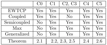
Table 2.1: MP-TCP algorithms

C0 C1 C2, C3 C4 C5

EWTCP Yes Yes Yes Yes Yes

Coupled Yes Yes No Yes Yes

Semicoupled No Yes Yes Yes Yes

Max No Yes Yes Yes Yes

Generalized No Yes Yes Yes Yes Theorem 2.1 2.2, 2.3, 2.5 2.4 2.6

2.2

Structural properties

Throughout this chapter we assume, for all xs, r ∈ s, s ∈S, kr(xs)> 0 and φr(xs) = 0 only if

xk =∞ for somek ∈s. A point (x,p) is called an equilibriumof (2.3)–(2.4) if it satisfies, for all

r∈s, s∈S andl∈L,

kr(xs) (φr(xs)−qr)

+

xr = 0

γl(yl−cl)

+

pl = 0

or equivalently,

xr≥0, φr(xs)≤qr and φr(xs) =qrifxr>0 (2.6)

pl≥0, yl≤cl and yl=clifpl>0. (2.7)

We make two remarks. First an equilibrium (x,p) does not depend onKs, but only on Φs. The design (Ks, s∈S), however, affects dynamic properties such as stability and responsiveness as we show below. Second, sincekr(xs)>0 andφr(xs) = 0 only ifxk =∞for somek∈sby assumption, any finite equilibrium (x,p) must haveqr>0 for allr. In the following we always restrict ourselves to finite equilibria.

(27)

2.2.1

Summary

We first present some properties of an MP-TCP algorithm (K,Φ) that we have identified. We then interpret them and summarize their implications.

C0: For each s∈S and eachxs, the Jacobians of Φs(xs) is continuous and symmetric, i.e.,

∂Φs

∂xs

(xs) =

_∂_Φ

s

∂xs (xs)

T .

C1: For each s ∈S there exists a nonnegative solution xs:= xs(p) to (2.6) for any finite p≥0 such thatqr>0 for allr. Moreover,

∂ys l(p)

∂pl

≤0, lim

pl→∞

ys_l(p) = 0,

where ys_l(p) :=P

r∈sHlrxr(p) is the aggregate traffic at linkl from sources.

C2: For each s∈ S and each xs, Φs(xs) is continuously differentiable; moreover, the symmetric part [∂Φs(xs)/∂xs]+ of the Jacobian is negative definite.

C3: For each r∈R,φr(xs) =∞if and only if xr= 0. The routing matrixH has full row rank. C4: For each r∈s,s∈S,P

j∈s[Ds]jr(xs)≤0, whereDs(xs) :=

h

∂Φs

∂xs(xs)

i−1

. C5: For each r∈R and eachx−r, limx_r→∞φr(xs) = 0.

These design criteria are intuitive and usually (but not always) satisfied; see Table 2.1.

Condition C0 guarantees the existence of utility functions Us(xs) that an equilibrium (x,p) of a multipath TCP/AQM (2.3)–(2.4) implicitly maximizes (Theorem 2.1). It is always satisfied when there is only a single path (|s|= 1 for alls) but not when|s|>1.

Conditions C1–C3 guarantee the existence, uniqueness, and global asymptotic stability of the equilibrium (x,p) (Theorems 2.2 and 2.3). C1 says that the aggregate traffic rate through a linkl

from sourcesdecreases when the congestion pricepl on that link increases, and it decreases to 0 as

pl increases without bounds. C2 implies that at steady state, ifxs,qs are perturbed by δxs, δqs, respectively, then (δxs)Tδqs<0. In the case of single-path TCP (|s|= 1 for alls), C2 is equivalent to the curvature of the utility function Us(xs) being negative, i.e., Us(xs) is strictly concave. C3 means that the rate on router is zero if and only if it sees infinite price on that route.

(28)

1T ∂xs

∂qr =

P

j∈sDjr at equilibrium for allr∈s. Thus C4 says that the aggregate throughput1Txs at equilibrium over all routesr∈sof an MP-TCP flow is a nonincreasing function of the priceqr.

Condition C5 is also satisfied by all the algorithms considered in this paper. It means that the sending rate on a route r grows unbounded when the congestion price qr is zero. Under C1–C3, an MP-TCP algorithm (K,Φ) is more responsive (see formal definition below) if the Jacobian of Φs(xs) is more negative definite (Theorem 2.5). C5 then implies an inevitable tradeoff: an MP-TCP algorithm that is more responsive is necessarily less TCP-friendly (Theorem 2.6).

We now elaborate on each of these properties.

2.2.2

Utility maximization

For single-path TCP (SP-TCP), one can associate a utility functionUs(xs)∈R+ →R with each

flows (xs is a scalar and|s|= 1) and interpret (2.3)–(2.4) as a distributed algorithm to maximize aggregate users’ utility, e.g. [47, 59, 62, 77]. Indeed, for SP-TCP, an (x,p) is an equilibrium if and only ifx is optimal for

maximize X s∈S

Us(xs) s.t. yl≤cl l∈L (2.8)

andpis optimal for the associated dual problem. Hereyl≤clmeans the aggregate trafficylat each link does not exceed its capacitycl. In fact this holds for a much wider class of SP-TCP algorithms than those specified by (2.3)–(2.4) [59]. Furthermore, all the main TCP algorithms proposed in the literature have strictly concave utility functions, implying a unique stable equilibrium.

The case of MP-TCP is much more delicate: whether an underlying utility function exists depends on the design choice of Φs and not all MP-TCP algorithms have one. Consider the multipath equivalent of (2.8):

maximize X s∈S

Us(xs) s.t. yl≤cl l∈L, (2.9)

wherexs:= (xr, r∈s) is the rate vector of flowsandUs:R|s|+ →Ris a concave function.

Theorem 2.1 (utility maximization). There exists a twice continuously differentiable and concave Us(xs)such that an equilibrium(x,p)of (2.3)–(2.4) solves (2.9)and its dual problem if and only if

condition C0 holds.

Condition C0 is satisfied trivially by SP-TCP when |s|= 1. For MP-TCP (|s|>1), the models derived in Section 2.1.2 show that only EWTCP and Coupled algorithms satisfy C0 and have under-lying utility functions. It therefore follows from the theory for SP-TCP that EWTCP has a unique stable equilibrium while Coupled algorithm may have multiple equilibria since its corresponding util-ity function is not strictly concave. The other MP-TCP algorithms all have asymmetric Jacobian

∂Φs

(29)

2.2.3

Existence, uniqueness and stability of equilibrium

Even though a multipath TCP algorithm (K,Φ) may not have a utility maximization interpretation, a unique equilibrium exists if conditions C1–C3 are satisfied.

Theorem 2.2 (existence and uniqueness). 1. Suppose C1 holds. Then (2.3)–(2.4) has at least one equilibrium.

2. Suppose C2 and C3 hold. Then (2.3)–(2.4) has at most one equilibrium

Thus (2.3)–(2.4) has a unique equilibrium(x∗,p∗)under C1–C3.

Conditions C1-C3 not only guarantee the existence and uniqueness of the equilibrium, they also ensure that the equilibrium is globally asymptotically stable, when the gainkr(xs) is only a function ofxritself, i.e.,kr(xs)≡kr(xr) for allr∈R. This is satisfied by all the existing algorithms presented in Section 2.1.2.

Theorem 2.3 (stability). Suppose C1-C3 hold and kr(xs) ≡ kr(xr) for all r ∈ R. Then the unique equilibrium (x∗_,_p∗₎_{is globally asymptotically stable. In particular, starting from any initial}

point x(0)∈R|R|+ and p(0)∈ R

|L|

+ , the trajectory (x(t),p(t))generated by the MP-TCP algorithm

(2.3)–(2.4) converges to the equilibrium(x∗,p∗)ast→ ∞.

Our proposed algorithm does not satisfy kr(xs)≡kr(xr) even though it seems to be stable in our experiments. This condition is only sufficient and needed in our Lyapunov stability proof; see Appendix 2.C. Whenkr(xs) depends onxs, one can replacekr(xr) in the definition of the Lyapunov functionV in (2.21) withkr(x∗_s) evaluated at the equilibrium and the same argument there proves that (x∗,p∗) is (locally) asymptotically stable. Also see Theorem 2.5 below for an alternative proof of local stability.

2.2.4

TCP friendliness

Informally, an MP-TCP flow is said to be ‘TCP friendly’ if it does not dominate the available bandwidth when it shares the same network with a SP-TCP flow [30]. To define this precisely we use the test network shared by a SP-TCP flow and a MP-TCP flow under test as shown in Fig. 2.1. All paths traverse a single bottleneck link with capacity c, with all other links with capacities strictly higher thanc. The links have fixed but possibly different delays. To compare the friendliness of two MP-TCP algorithms ˆM := ( ˆK,Φ) and ˜ˆ M := ( ˜K,Φ), suppose that when ˆ˜ M shares the test network with a SP-TCP it achieves a throughput ofkxˆk1in equilibrium aggregated over the available

paths (the SP-TCP therefore attains a throughput ofc− kˆxk1). Suppose ˜M achieves a throughput

ofkx˜k1in equilibrium when it shares the test network with the same SP-TCP. Then we say that ˆM

isfriendlier (or more TCP-friendly)than ˜M ifkxˆk1≤ kx˜k1, i.e., if ˆM receives no more bandwidth

(30)

c

MP-TCP

Flow MP-TCPFlow

SP-TCP

Flow SP-TCPFlow

Figure 2.1: Test network for the definition of TCP friendliness. The link in the middle is the only bottleneck link with capacityc.

From the theory for single-path TCP (|s|= 1 for all s∈ S), it is known that a design is more TCP-friendly if it has a smaller marginal utility U_s0(xs) = Φs(xs). The same intuition holds for MP-TCP algorithms even though the utility functions may not exist for MP-TCP algorithm.

Theorem 2.4 (friendliness). Consider two MP-TCP algorithms Mˆ := ( ˆK,Φ)ˆ and M˜ := ( ˜K,Φ)˜ . Suppose both satisfy C1–C4. ThenMˆ is friendlier thanM˜ ifΦs(ˆ xs)≤Φs(˜ xs)for all s∈S.

2.2.5

Responsiveness around equilibrium

Suppose conditions C1–C3 hold and there is a unique equilibriumz∗:= (x∗,p∗). Assume all links in

Lare active withp∗_l >0; otherwise remove fromLall links with pricesp∗_l = 0. Letδz(t) :=z(t)−z∗. The behavior of (2.3)–(2.4) around the equilibrium is defined by the linearized system:

δz˙ = J∗ δz(t). (2.10)

HereJ∗ is the Jacobian of (2.3)–(2.4) at the equilibriumz∗:

J∗ := J(x∗) :=





Λk∂_∂Φ_x −ΛkHT

ΛγH 0



,

where Λk=diag{kr(x∗_s), r∈R}, Λγ =diag{γl, l∈L}, and ∂_∂Φ_x is evaluated atx∗.

The stability and responsiveness of the linearized system (2.10) (how fast does the system con-verges to the equilibrium locally) is determined by the real parts of the eigenvalues ofJ∗. Specifically the linearized system is stable if the real parts of all eigenvalues of J∗ _{are negative; moreover the} more negative the real parts are the faster the linearized system converges to the equilibrium. We now show that the linearized system (2.10) is stable (i.e., converges exponentially fast toz∗ locally) and characterize its responsiveness in terms of the design choices (K,Φ).

LetZ ={z:= (x,p)∈_C|R|+|L|_{| k}_z_k

2= 1}.

(31)

1. The linearized system (2.10) is stable, i.e., Re(λ)<0 for any eigenvalue λof J∗. Moreover

Re(λ)≤λ(J∗), where

λ(J∗) := max z∈Z

(

xH∂_∂Φ_x+x xH_Λ−1

k x+pHΛ −1

γ p

)

≤ 0,

where Λk and ∂Φs

∂xs are evaluated at the equilibrium pointz

∗_.

2. For two MP-TCP algorithms( ˆK,Φ)ˆ and( ˜K,Φ)˜ ,λ( ˆJ∗)≤λ( ˜J∗)provided

ˆ

Ks ≥ K˜s and

∂Φsˆ

∂xs

∂Φs˜ ∂xs

for alls∈S.

Theorem 2.5 motivates the following definition of responsiveness. Given two MP-TCP ˆM and ˜

M, we say that ˆM is more responsive than M˜ ifλ( ˆJ∗)≤λ( ˜J∗). Theorem 2.5(2) implies that an MP-TCP algorithm with a largerKs(x∗_s) or more negative definiteh∂Φs

∂xs(x

∗ s)

i+

is more responsive, in the sense that the real parts of the eigenvalues of the JacobianJ∗ have a smaller more negative upper bound.

Then the next result suggests an inevitable tradeoff between responsiveness and friendliness.

Theorem 2.6 (tradeoff). Consider two MP-TCP algorithms(K,Φ)ˆ and(K,Φ)˜ with the same gain K. Suppose both satisfy C1-C3 and C5. Then for alls∈S

∂Φs(ˆ xs)

∂xs

∂Φs(˜ xs) ∂xs

⇒ Φs(ˆ xs) ≥ Φs(˜ xs).

In light of Theorems 2.4 and 2.5, Theorem 2.6 says that a more responsive MP-TCP design is inevitably less friendly if they have the sameK.

The theorem is easier to understand in the case of SP-TCP, i.e., when |s|= 1 for alls∈S and Φs(xs) =U_s0(xs). Then it implies that a more concave utility functionUs(xs) has a larger marginal utility, and is hence less friendly.

2.2.6

Window oscillation

Window oscillations are inherent in loss-based additive increase multiplicative decrease (AIMD) TCP algorithms. We close this section by discussing informally why a larger designKs(xs) generally creates more severe window oscillations. This implies a tradeoff between responsiveness (which is enhanced by a largeKs(xs)) and oscillation (which is reduced with a smallKs(xs)).

The effect of Ks(xs) on window fluctuations can be understood by studying how it affects the decreaseDr(ws) per packet loss in the following packet level model:

(32)

• For each loss on router,wr←wr−Dr(ws).

Let Zr ∈ {0,1} be an indicator variable of whether a packet loss is observed on route r at an arbitrary time in steady state. Then

Ds(xs) := 1

kxsk1

E X

r∈s

Dr(ws)

τr Zr X k∈s

Zk≥1

!

.

represents the expected relative reduction inaggregatethroughputP

r∈sDr(ws)/τr, given that there is at least one packet loss on some route r∈s. It is a measure of throughput fluctuation for each packet loss that an application experiences. For TCP-NewReno (for which s = {r} and ws is a scalar), the window size is halved on each packet loss,Dr(ws) =wr/2, and hence Ds(xs) = 1/2.

To understand Ds(xs) for MP-TCP algorithms, we need the following result.

Lemma 2.7. LetAi:={ai1, ai2, . . .}with|Ai|elements. Each elementaij is an independent binary

random variable with P(aij= 1) = 1−P(aij = 0) =qi. Define Di(Ai) :=di1(P

jaij≥1). Then

E



 X

k

Dk(Ak)

X i,j

aij ≥1



 = P

kdkqk|Ak|

P

kqk|Ak|

+o X

k

qk

!

.

Suppose each route has a fixed loss probability qr. Then within each RTT, Lemma 2.7 implies

Ds(xs) = 1

kxsk1

P

r∈swrqrDr(ws)/τr

P

r∈sqrwr

+o X

r∈s

qr

!!

.

Substitutingwr=xrτrandxrDr(ws) =τrkr(xs) from (2.5), we get, ignoring the high-order terms,

Ds(xs) = 1

kxsk1

P

r∈sτrqrkr(xs)

P

r∈sτrqrxr

. (2.11)

to the first order. Note that kr(xs) does not affect the equilibrium rates xs. Hence, with the assumption thatτr are constants,Ds(xs) is determined by the functionskr(xs) in steady state.

Specifically an MP-TCP algorithm with a larger Ks(xs) tends to have a larger Ds(xs) and hence more severe window oscillations. Theorem 2.5, however, suggests that a larger Ks(xs) also leads to better responsiveness, suggesting an inevitable tradeoff between responsiveness and window oscillation.

2.3

Implications and a new algorithm

(33)

discussion motivates a new design that generalizes the existing MP-TCP algorithm.

2.3.1

Implications on existing algorithms

Recall Table 2.1 that summarizes the conditions satisfied by the various algorithms. Only EWTCP and Coupled algorithms satisfy C0. Their equilibrium properties can be studied in the standard utility maximization model as done for single-path TCP. Semicoupled and Max algorithms do not satisfy C0 and therefore analysis through utility maximization is not applicable. However, Theorem 2.8 below implies that both Semicoupled and Max algorithms satisfy C1–C3 provided they enable no more than 8 routes. Theorem 2.2 and 2.3 then imply that they have a unique and globally stable equilibrium. It is also easy to show that EWTCP satisfies C1-C3. The Coupled algorithm does not satisfy C2 and is found to have multiple equilibria in [46].

Next we discuss friendliness of existing MP-TCP algorithms. It can be shown that the φr(xs) corresponding to these algorithms satisfy:

φewtcpr (xs)≥φ

semicoupled

r (xs)≥φ max

r (xs)≥φ coupled r (xs)

for all xs ≥ 0 if all routes r ∈ s have the same round trip time. Since all of them satisfy C4, Theorem 2.4 implies that their friendliness will be in the same order, i.e., their throughputs in the test network of Fig. 2.1 are ordered as follows:

EWTCP(a≥1)1≥Semicoupled≥Max≥Coupled. This is confirmed by the Linux-based experiment.

Third we will discuss responsiveness of existing MP-TCP algorithms. These algorithms have the same gain functionkr(xs) = 0.5x2r and

(∂Φs

∂xs

)ewtcp(∂Φs

∂xs

)semicoupled (∂Φs

∂xs

)max(∂Φs

∂xs

)coupled.

Theorem 2.5 then implies that their responsiveness should be in the same order, as confirmed by our experiments in section 2.4.

Finally we discuss window oscillation of existing MP-TCP algorithms usingDs(xs) as the metric. As mentioned in Section 2.2.6, Ds(xs) = 0.5 for TCP NewReno, a benchmark single-path TCP algorithm. According to (2.11), ifkr(xs)≤0.5xrkxsk1, we have, to the first order

Ds(xs) ≤ 1

2

P

r∈sτrqrxrkxsk1

kxsk1P_r∈sτrqrxr = 1

2.

1_When_{a <} _{1, the MP-TCP source can obtain even smaller throughput than the competing single-path TCP}

(34)

All existing MP-TCP algorithms have the samekr(xs) = 0.5x2r≤0.5xrkxsk1, with strict inequality

if|s|>1 andxr>0 for at least twor∈s. Thus enabling MP-TCP always tends to reduce window oscillation for existing algorithms compared to TCP NewReno. Moreover, the window oscillation is always reduced compared to TCP NewReno whenkr(xs)≤0.5xrkxsk1.

2.3.2

A generalized algorithm

Consider the class of algorithms parametrized by (β, n, η) as follows:







kr(xs) =1₂xr(xr+η(kxsk∞−xr)), η≥0

φr(xs) =

2((1−β)xr+βkxskn)

τ2

rxrkxsk21

, n∈_N+, β≥0

. (2.12)

This class includes the Max (β = 1, η = 0, n = ∞), Coupled (β = 0, η = 0), and Semicoupled (β = 1, η = 0, n = 1) algorithms as special cases when all RTTs on different paths of the same source are the same, i.e.,τr=τs,r∈s.

The next result characterizes a subclass that have a unique and locally stable equilibrium point.

Theorem 2.8. Fix anyη ≥0 andn∈N+. For anys∈S, the φr(xs)in (2.12)satisfies

1. C1 ifβ≥0.

2. C2–C3 if0< β ≤1,|s| ≤8andτrare the same for allr∈s(assumingH has full row rank). The requirement that |s| ≤8 is not restrictive since in practice a device may typically enable no more than 3 paths. The requirement that τr are the same for all r ∈s is used in proving the negative definiteness of the (symmetric part of the) Jacobian of Φs(xs). Since a negative definite matrix remains negative definite after small enough perturbations of its entries, Theorem 2.8 holds if the RTTs of the subpaths do not differ much. This (sufficient) condition seems reasonable as two paths between the same source-destination pair often have similar RTTs if both are wireline paths. Note that our experiments in chapter 2.4 show that the algorithm also converges even if the RTTs on different paths differ dramatically, e.g. the RTT of WiFi is usually much smaller than that of 3G.

For the class of algorithms specified by (2.12), Theorem 2.8 motivates a design space defined by

β ∈(0,1], η ≥0, n∈_N+, where β andn control the tradeoff between friendliness and

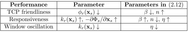
responsive-ness and η controls the tradeoff between responsiveness and window oscillation. In Table 2.2, we summarize how the parameters (β, η, n) affect the performance.

(35)

Table 2.2: How design choices affect MP-TCP performance.

Performance Parameter Parameters in (2.12)

TCP friendliness φr(xs)↓ β↓, n↑

Responsiveness kr(xs)↑,−∂Φs/∂xs↑ β ↑,n↓,η↑

Window oscillation kr(xs)↓ η↓

Jacobian [∂Φs/∂xs]+ (Theorem 2.5). However, a largerKs usually creates a bigger window oscilla-tion; a more negative definite [∂Φs/∂xs]+implies a larger Φs, usually hurting friendliness (Theorems 2.6 and 2.4). This is summarized in Table 2.2. Since enabling multiple paths already reduces win-dow oscillation compared to single-path TCP (section 2.3.1), MP-TCP can afford to use a relatively large gainKs for responsiveness. This does not compromise too much on window oscillation, but allows us to use a less negative definite Jacobian [∂Φs/∂xs]

+

with a smaller Φsto maintain sufficient TCP friendliness. Moreover, responsiveness is mainly affected by subpaths with small throughput while window oscillation is mainly affected by subpaths with large throughput. The parameter η

in the generalized algorithm (2.12) scaleskr(xs) in the right way: a pathrthat has a largexrhas

kr(xs)≈0.5x2

rand hence a similar degree of window oscillation as existing algorithms, while a path

r with a small xr has larger kr(xs) than that under a design with zero η and therefore is more responsive.

Our experiments show that Max algorithm ((β, η, n) = (1,0,∞)) overtakes too much of the competing single-path TCP flows. Therefore, we can only use a smallerβ sincenis already infinite in order to improve friendliness. To compensate for the responsiveness performance, we will use a larger η, which will sacrifice window oscillation performance. The Balia MP-TCP algorithm given at the beginning of this chapter corresponds to the choice (β, η, n) = (0.2,0.5,∞). Instead of allowing the window size to drop to 1 for a packet loss, we add a cap for the decrement of window size, which improves the performance as confirmed in our experiments. Note that there is no “best” parameter setting since there are tradeoffs among all the performance metrics and we choose (β, η, n) = (0.2,0.5,∞) based on our experiments in chapter 2.4, which show that this parameter setting strikes a good balance among responsiveness, friendliness, and window oscillation.

2.4

Experiment

(36)

Figure 2.2: Network for our Linux-based experiments on TCP friendliness and responsiveness, with

N1 MP-TCP flows andN2 single-path TCP flows sharing two links of capacity, c1, c2, and

propa-gation delay (single trip) T1,T2. MP-TCP flows maintain two routes with ratex1, x2. Single-path

TCP flows maintain one route with ratex3.

instead of 2 when more than 1 path is available.

The network topology is shown in Fig. 2.2. In the testbed, all nodes are Linux machines with a quad-core Intel i5 3.33GHz processor, 4GB RAM, and multiple 1Gbps Ethernet interfaces, running Ubuntu 13.10 (Linux kernel 3.11.8). The network parameters such asc1,c2,T1, andT2are controlled

by Dummynet [13].

Our experiments are divided into three parts. First we compare TCP friendliness of Balia algorithm and prior algorithms. The result confirms that the Couple algorithm is the friendliest, and that the Balia algorithm is close to the Coupled algorithm and friendlier than the other algorithms. Second, we compare the responsiveness of each algorithm in a dynamic environment where flows come and go. The result shows that the Coupled and OLIA algorithms are unresponsive (illustrating the tradeoff between responsiveness and friendliness). EWTCP is the most responsive; Balia is similar in responsiveness but friendlier to single-path TCP flows. Finally we show that all MP-TCP algorithms have smaller average window oscillations than single-path TCP.

These experiments confirm our analytical results and suggest our design choice strikes a good balance among friendliness, responsiveness, and window oscillation.

2.4.1

TCP friendliness

We study TCP friendliness of each algorithm, first with paths of similar RTTs and then with paths of different RTTs, which emulates the wireless scenario. We assume all the flows are long lived and focus on the steady state throughput.

In the first set of experiments, we letT1=T2= 5ms,c1=c2= 60Mbps andN1=N2= 30. We

(37)

0 20 40 60 80 100 120

0 40 80 120 160

cwnd Time (s) EWTCP MP-Subpath1 MP-Subpath2 0 10 20 30 40

0 40 80 120 160

Throughput (Mbp s) Time (s) EWTCP MP-TCP SP-TCP 0 20 40 60 80 100 120

0 40 80 120 160

cwnd Time (s) Semicoupled MP-Subpath1 MP-Subpath2 0 10 20 30 40

0 40 80 120 160

Throughput (Mbp s) Time (s) Semicoupled MP-TCP SP-TCP 0 20 40 60 80 100 120

0 40 80 120 160

cwnd Time (s) Max MP-Subpath1 MP-Subpath2 0 10 20 30 40

0 40 80 120 160

Throughput (Mbp s) Time (s) Max MP-TCP SP-TCP 0 20 40 60 80 100 120

0 40 80 120 160

cwnd Time (s) Balia MP-Subpath1 MP-Subpath2 0 10 20 30 40

0 40 80 120 160

Throughput (Mbp s) Time (s) Balia MP-TCP SP-TCP 0 20 40 60 80 100 120

0 40 80 120 160

cwnd Time (s) Coupled MP-Subpath1 MP-Subpath2 0 10 20 30 40

0 40 80 120 160

Throughput (Mbp s) Time (s) Coupled MP-TCP SP-TCP 0 20 40 60 80 100 120

0 40 80 120 160

cwnd Time (s) OLIA MP-Subpath1 MP-Subpath2 0 10 20 30 40

0 40 80 120 160

Throughput (Mbp s) Time (s) OLIA MP-TCP SP-TCP

Figure 2.3: Responsiveness Performance: congestion window trajectory of MP-TCP for each path (left column). SP-TCP starts at time 40s and ends at 80s. The throughput of SP-TCP and total throughput of MP-TCP are shown in the right column. Parameters: T1 =T2 = 10ms, c1 =c2 =

(38)

Table 2.3: TCP friendliness (same RTTs): Average throughput (Mbps) and 95% confidence interval of MP-TCP and single-path TCP users. (T1=T2= 5ms,c1=c2= 60Mbps andN1=N2= 30)

ewtcp semi. max balia coupled olia mp-tcp

(throuput) 2.75 2.65 2.60 2.52 2.44 2.61 mp-tcp

(CI) 0.005 0.004 0.005 0.006 0.005 0.004 sp-tcp

(throuput) 0.951 1.07 1.13 1.22 1.29 1.12 sp-tcp (CI) 0.005 0.007 0.008 0.006 0.005 0.004

In the second set of experiments, we assume a highly heterogeneous RTTs by emulating the scenario of a mobile device with both 3G and WiFi access. WiFi access usually has higher capacity and lower delay compared to 3G. Specificially, we setT1 = 10ms, c1 = 8Mbps for the first link to

emulate WiFi access andT2= 100ms,c2= 2Mbps for the second link to emulate 3G access. When

there exists single-path TCP flows, i.e. N2 >0, the behaviors of all the algorithms are similar to

the equal RTT case in the first set of simulation. The Coupled algorithm is the friendliest and the Balia algorithm is closer than other algorithms. However, when there is no single-path TCP flow, i.e. N1 = 1 and N2 = 0, the performance of OLIA is not stable enough to effectively take all the

available capacity while the other algorithms do not have such problem. We repeat the experiments 20 times and we find that sometimes OLIA does not use the 3G access link. The average throughput of MP-TCP user and the 95% margin of error for confidence interval is shown in Table 2.4.

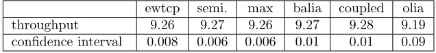
Table 2.4: Basic behavior (WiFi/3G): throughput (Mbps) of a MP-TCP user and 95% confidence interval. (T1= 10ms,T2= 100ms,c1= 8Mbps,c2= 2Mbps,N1= 1, N2= 0)

ewtcp semi. max balia coupled olia

throughput 9.26 9.27 9.26 9.27 9.28 9.19

confidence interval 0.008 0.006 0.006 0.01 0.01 0.09

2.4.2

Responsiveness

We use the network in Fig. 2.2 withc1 =c2 = 20Mbps,T1 =T2 = 10ms andN1 = 1, N2 = 5. To

demonstrate the dynamic performance of each algorithm, we assume the MP-TCP flow is long lived while the single-path TCP flows start at 40s and end at 80s. We record the aggregate throughput of the single-path TCP flows from 40-80s, which measures the friendliness of MP-TCP. We also measure the time for the congestion window on the second path to recover2 of MP-TCP users. It measures the responsiveness of MP-TCP. These measurements are shown in Table 2.5 and the congestion window and throughput trajectories of all algorithms are shown in Fig. 2.3. To clearly show the

2_{Defined as the first time the congestion window on the second path reaches the average congestion window (e.g.,}

(39)

responsiveness performance, we record the longest convergence time found in our experiment in Table 2.5 and the corresponding trajectories are shown in Fig. 2.3.

Table 2.5: Responsiveness: convergence time (s) of MP-TCP and total throughput (Mbps) of all single-path TCP users. (T1=T2= 10ms, c1=c2= 20Mbps,N1= 1, N2= 5)

ewtcp semi. max balia coupled olia Convergence 3.25 7.46 17.75 14.73 94.36 58.5 SP-TCP 13.89 15.35 15.8 16.28 16.64 16.97

EWTCP is the most responsive among all the algorithms. Ours is as responsive as the Max algorithm, yet significantly friendlier than EWTCP. Both Coupled and OLIA algorithms take an excessively long time to recover. For Coupled algorithm, the excessively slow recovery of the conges-tion window on the second path (see Fig. 2.3) is due to the design that increases the window roughly bywr/(P_k∈swk)2 on each ACK, assuming the RTTs are similar. After the single-path TCP flow has left,w2 is small whilew1is large, so thatw2/(w1+w2)2is very small. It therefore takes a long

time for w2 to increase to its steady state value. In general, under the Coupled algorithm, a route

with a large throughput can greatly suppress the throughput on another route even though the other route is underutilized. The reason of the poor responsiveness performance of OLIA can be explained using a similar argument to the Coupled algorithm since they have the same increment/decrement for each ACK/loss in this scenario.

0 10 20 30 40 50 60

0 20 40 60 80 100

cwnd

Time (s)

Balia

Subpath1 Subpath2 Total

0 10 20 30 40 50 60

0 20 40 60 80 100

cwnd

Time (s)

Linux TCP (Reno)

TCP-Reno

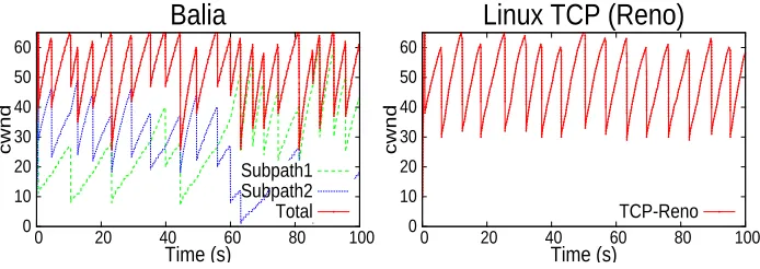
Figure 2.4: Window oscillation: the red trajectories represent throughput fluctuations experienced by the application in the case of MP-TCP and the case of single-path TCP.

2.4.3

Window oscillation

(40)

enabling multiple paths reduces the average window oscillation compared with only using a single path.

2.5

Conclusion

(41)

Appendix

2.A

Proof of Theorem 2.1 (utility maximization)

The Lagrangian of (2.9) is:

L(x,p) =X s∈S

Us(xs)−X

l∈L

pl(yl−cl)

=X

s∈S

Us(xs)−X

l∈L

pl(X r∈R

Hlrxr−cl)

=X

s∈S

Us(xs)−

X

r∈s

xrqr

!

+X

l∈L

plcl,

wherep≥0are the dual variables andqr:=P_r∈RHlrpl. Then the dual problem is

D(p) =X s∈S

max xs≥0

{Bs(xs,p)}+

X

l∈L

plcl p≥0,

whereBs(xs,p) =Us(xs)−P_r∈sxrqr. The KKT condition implies that, at optimality, we have

∂Us(xs)

∂xr

< qr⇒xr= 0 andxr>0⇒

∂Us(xs)

∂xr

=qr (2.13)

yl< cl⇒pl= 0 and pl>0⇒yl=cl. (2.14)

Comparing with (2.6)–(2.7) we conclude that, if a MP-TCP algorithm defined by (2.3)–(2.4) has an underlying utility functionUs, then we must have

∂Us(xs)

∂xr

=φr(xs) r∈s, xr>0. (2.15)

Givenφr(xs), (2.15) has a continuously differentiable solutionsUs(xs) if and only if the Jacobian of Φs(xs) is symmetric, i.e., if and only if

∂Φ(xs)

∂xs =

∂Φ(xs)

∂xs

(42)

2.B

Proof of Theorem 2.2 (existence and uniqueness)

2.B.1

Proof of part 1

For any linkl∈L, let

p−l={p1, . . . , pl−1, pl+1, . . . , p|L|},

whose component composes of all the elements inpexceptpl. Forl∈L, let

gl(p) :=cl−

X

r:l∈r

xr=cl−

X

s:r∈s,l∈r

ys_l(pl,p−l)

andhl(p) :=−gl2(p). According to C1, we have the following two facts, which will be used in the proof.

• gl(p) is a nondecreasing function of pl onR+ sinceyls(p) is a nonincreasing function ofpl.

• limp_l→∞gl(pl,p−l) =clsince limpl→∞y

s

l(p) = 0.

Next, we will show that hl(p) is a quasi-concave function of pl. In other words, for any fixed

p−l, the set Sa:={pl|hl(p)≥a} is a convex set. Ifgl(0,p−l)≥0, then

gl(pl,p−l)≥gl(0,p−l)≥0 ∀pl≥0,

which meanshl(pl,p−l) is a nonincreasing function ofpl, and hence is a quasi-concave function of

pland

arg max pl

hl(pl,p−l) = 0. (2.16)

On the other hand, ifgl(0,p−l)<0, then there exists ap∗_l >0 such thatgl(p∗_l,p−l) = 0 since gl(·) is continuous and limp_l→∞gl(pl,p−l) =cl >0. Note that gl(p) is a nondecreasing function of pl, thenhl(pl,p−l) is nondecreasing forpl∈[0, p∗l] and nonincreasing forpl∈[p∗l,∞). Thus,hl(pl,p−l) is also a quasi-concave function ofpl in this case and

max pl

hl(pl,p−l) = 0. (2.17)

By Nash theorem, ifhl(pl,p−l) is a quasi-concave function ofplfor alll∈Landpis in a bounded set, then there exists ap?_∈

R|L|+ such that

p?l = arg max pl∈R+

hl(pl,p∗−l).

(43)

time. Thereforep∗ satisfies Eqn. (2.7). Since q =RT_p_{, there exists an}_x∗ _{to (2.6). Thus there} exists at least one solution (x,p) that satisfies (2.6) and (2.7).

2.B.2

Proof of part 2

Lemma 2.9. Assume a function F : Rn → Rn is continuously differentiable and ∂F∂x(x)

+ is

negative definite for allx. Then for anyx16=x2∈Rn,

(x1−x2)T(F(x1)−F(x2))<0.

Proof. Fix anyx16=x2∈Rn. DefineA(t) :=F(tx1+ (1−t)x2). Since∂F/∂xis continuous, there

exists a λ <0 such that the eigenvalues of [∂F/∂x]+ _≤_λ_{over the compact set}_{_t_x

1+ (1−t)x2 |

0≤t≤1}. Then

(x1−x2)T(F(x1)−F(x2))

=

Z 1

0

(x1−x2)T

dA dt(τ)dτ

=

Z 1

0

(x1−x2)T

∂F

∂x(τx1+ (1−τ)x2) (x1−x2)dτ

≤ λkx1−x2k22<0.

Lemma 2.10. Suppose C3 holds. Then x∗_r>0 at equilibrium for allr∈R.

Proof. Supposex∗_r= 0. Thenq∗_r≥φr(x∗r) =∞by C3 and hence there is a linkl∈rwith p∗l =∞. But then, for all paths r0 3 l, q∗_r0 =∞ and hence x∗_r0 = 0 by C3. This implies y∗_l = 0< cl, and

hencep∗_l = 0 by (2.7), contradictingp∗_l =∞.

Recall the vector notations that x:= (xs, s∈S) := (xr, r∈s, s∈S) and Φ(x) := (Φs(xs), s∈

S) := (Φr(xs), r ∈ s, s ∈ S). To prove uniqueness of the equilibrium, suppose for the sake of contradiction that there are two distinct equilibrium points (x,p) and (ˆx,pˆ). By Lemma 2.10 we have x>0 and ˆx>0. Thus (2.6) implies Φ(x) =q=HTpand Φ(ˆx) = ˆq=HTpˆ. By Lemma 2.9 and assumption C2 we then have

(44)

Thus

pTy+ ˆpTyˆ < pTyˆ+ ˆpTy. (2.18)

Equilibrium condition (2.7) implies

pT(c−y) = 0 and pˆT(c−yˆ) = 0 (2.19)

y ≤ c and yˆ ≤ c. (2.20)

Substituting (2.19) into (2.18) yields

pTc+ ˆpTc < pTyˆ+ ˆpTy pT(c−yˆ) + ˆpT(c−y) < 0.

But (2.20) implies that the left-hand side of the last inequality is nonnegative (sincep≥0, ˆp≥0), which is a contradiction. Therefore the equilibrium is unique.

2.C

Proof of Theorem 2.3 (stability)

We will construct a Lyapunov function and use LaSalle’s invariance principle [49] to prove global asymptotic stability of the unique equilibrium point (x∗,p∗). Defineδx:=x−x?_, _δ_p_:=_p₋_p?_. Consider the candidate Lyapunov function:

V(x,p) =X r∈R

Z xr

x∗

r

z−x∗ r

kr(z) dz+ 1 2

X

l∈L

δp2

l

γl

. (2.21)

By definition,V(x,p)>0 for all (x,p)6= (x∗,p∗) andV(x,p) = 0 if (x,p) = (x∗,p∗). Furthermore

V is radially unbounded, i.e.,V(x,p)→ ∞ask(x,p)k2→ ∞. Finally

˙

V(x,p) =X r∈R

1

kr(xr)

δxrx˙r+

X

l∈L 1

γl

δplp˙l.

Ifδxr6= 0 then we have (since kr(xs) =kr(xr)) 1

kr(xr)δxrx˙r = δxr(φr(xs)−qr)

+

xr

≤ δxr(φr(xs)−qr)

(45)

The first inequality holds since (φr(xs)−qr)+xr =φr(xs)−qrifxr>0 andφr(xs)−qr≤0,δxr=−x

∗ r ifxr= 0. The last equality holds sinceφr(x∗s) =qr∗ by Lemma 2.10 and (2.6). Therefore

X

r∈R 1

kr(xr)δxrx˙r ≤ δx T

(Φ(x)−Φ(x∗))−δxTδq

< −δxTHTδp,

where the last inequality holds since δxT₍_φ₍_x₎₋_φ₍_x∗₎₎ _< _{0 by Lemma 2.9 and assumption C2.} Similarly

1

γl

δplp˙l = δpl(yl−cl)+pl ≤ δpl(yl−cl) ≤ δplδyl,

where the last inequality holds sinceδplcl≥δplyl∗ by the equilibrium condition (2.7). Thus

X

l∈L 1

γl

δplp˙l ≤ δpTHδx.

Therefore ifδx6= 0 then

˙

V(x,p) < −δxTHTδp+δpTHδx = 0

and ifδx= 0 then ˙V(x,p) = 0. This means ˙V(x,p)≤0 andV is indeed a Lyapunov function. Consider the set

Z := { (x(t),p(t))|V˙(x(t),p(t)) = 0 for allt≥0}

of trajectories on which ˙V ≡0. If the only trajectory inZ is the trivial trajectory (x,p)≡(x∗,p∗) then LaSalle’s invariance princ

Distributed Control and Optimization for Communication and Power Systems