Volume 2009, Article ID 909636,14pages doi:10.1155/2009/909636
Research Article
Iterative PSF Estimation and Its Application to Shift Invariant
and Variant Blur Reduction
Seung-Won Jung,
1Byeong-Doo Choi,
2and Sung-Jea Ko
11Department of Electronics Engineering, Korea University, Anam-Dong, Sungbuk-Ku, Seoul 136-701, South Korea 2Fraunhofer Institute for Telecommunications, Heinrich-Hertz-Institut (HHI), 10587 Berlin, Germany
Correspondence should be addressed to Sung-Jea Ko,[email protected]
Received 16 February 2009; Accepted 8 October 2009
Recommended by Stephen Marshall
Among image restoration approaches, image deconvolution has been considered a powerful solution. In image deconvolution, a point spread function (PSF), which describes the blur of the image, needs to be determined. Therefore, in this paper, we propose an iterative PSF estimation algorithm which is able to estimate an accurate PSF. In real-world motion-blurred images, a simple parametric model of the PSF fails when a camera moves in an arbitrary direction with an inconsistent speed during an exposure time. Moreover, the PSF normally changes with spatial location. In order to accurately estimate the complex PSF of a real motion blurred image, we iteratively update the PSF by using a directional spreading operator. The directional spreading is applied to the PSF when it reduces the amount of the blur and the restoration artifacts. Then, to generalize the proposed technique to the linear shift variant (LSV) model, a piecewise invariant approach is adopted by the proposed image segmentation method. Experimental
results show that the proposed method effectively estimates the PSF and restores the degraded images.
Copyright © 2009 Seung-Won Jung et al. This is an open access article distributed under the Creative Commons Attribution License, which permits unrestricted use, distribution, and reproduction in any medium, provided the original work is properly cited.
1. Introduction
Due to the degradation of the image caused by the limited performance of optical and electronic devices of in today’s cameras, the image restoration has been researched in literature. In classical image restoration, the PSF is assumed to be known prior to the restoration process [1]. However, in real-world applications, an observed image is only available with insufficienta prioriinformation.
Various techniques have been proposed to estimate the PSF. Early works on blur identification, or the estimation of the PSF, have been proposed based on regular patterns of zeros in the frequency domain [2]. However, these methods are sensitive to Gaussian blur that does not have zeros in the frequency domain. To deal with this problem, the spatial domain Bayesian parameter estimation of the PSF has been widely adopted [3,4]. Especially in the case of motion blur, the PSF is assumed to be modeled as a uniform motion blur. Then, the parameters of the uniform motion blur, the length and angle, are estimated with an optimization technique. Though these approaches estimate an accurate PSF, they
are not applicable to the PSF which cannot be regarded as a parametric form. In many real applications, the camera tends to move in a nonlinear direction with acceleration. Therefore, the parametric estimation of the PSF sometimes yields unsatisfactory result, so that the deblurred image tends to have restoration artifacts. In this case, the parametric PSF estimation needs to be revised to estimate a more accurate PSF.
image only into blurred and not blurred regions [7] or use a well-known image segmentation method for the object-based processing [9]. However, since a blurred region may not have a homogeneous PSF, a single PSF for the blurred region cannot accurately describe the blur of the image. Also, the conventional image segmentation methods are not efficient for image deblurring because they generally over-segment images without considering the image blur.
In this paper, we first divide an image into multiple segments where each segment can be assumed to be blurred by the LSI PSF. Then, the LSI PSF is estimated by the proposed PSF estimation algorithm. To estimate the PSF, spreading operators are employed when they increase the accuracy of the PSF. The accuracy of the PSF is assessed by a cost function, which measures both the blur strength and undesired artifacts. Finally, image deconvolution is performed for each segment by using the estimated LSI PSF. By merging all of the resultant segments, we can obtain the deblurred image.
The rest of this paper is organized as follows. We describe the proposed PSF estimation method in Section 2
and show how to measure the amount of blurs and artifacts in Section 3. The application to the shift variant model is presented inSection 4. Experimental results and conclusion are given inSection 5andSection 6, respectively.
2. Proposed Directional Spreading of the PSF
Before introducing the proposed method, it is worth clar-ifying the motivation for the proposed method. In image restoration, the image degradation [10] is generally modeled as
g=h∗f +n, (1)
where f,g,h, andndenote the original image, the observed image, the PSF, and the observation noise, respectively. Given h, f can be reconstructed from g by using image deconvolution algorithms [10]. However, the PSF needs to be estimated since the PSF cannot be known in real motion-blurred images. In the LSI model, the PSF is assumed to be invariant for a whole image. Then, the invariant PSF of the image is estimated by conventional techniques [2,4]. Since most of the conventional approaches rely on a parametric model of the PSF, their estimation accuracies are dependent on the reliability of the model. Especially for the case of motion blur, the uniform motion blur model is widely adopted. However, when the camera moves to an irregular direction within an exposure time, the uniform motion blur model fails to estimate an accurate PSF. As can be seen fromFigure 1, the original PSF shaped asFigure 1(a)cannot be estimated by the uniform motion blur model shown in
Figure 1(b). In Figure 1, + indicates a center position of the PSF and the grey value represents a magnitude of the PSF at the corresponding coefficient. The coefficient values of the PSF vary from 0 to 1, so those values are linearly mapped from 0 to 255 for the visualization. Since image deconvolution is inherently an ill-conditioned problem, the inaccurate PSF may cause serious artifacts in the resultant
image. Therefore, in this section, we present an iterative PSF estimation technique that modifies the initial PSF at each iteration.
Figure 1(c) conceptually illustrates the expected result of the proposed method. As can be seen, the directional spreading operator can be applied to update the initial PSF for improving the accuracy of the PSF. The decision rule of applying the directional spreading operator will be explained in the next section. Given a certain decision rule, it is obvious that the estimation performance depends on the design of the spreading operator.
In this paper, we use four directional filters to spread the PSF since the combination of the four directional spreading can closely approximate the other directions.Figure 2shows an example of directional filters whose size is 5×5. At the previous example inFigure 1, these spreading operators are applied to the initial PSF of 64×64 size for the graphical explanation. Then, let a set of spreading operators be denoted as S = {s0,s1,s2,s3}. Each operator in S represents 1D finite impulse response (FIR) filter of four directions, that is, upper, lower, left, and right. For instance, the impulse response of the left and right directional filters,s2ands3, are defined by
s2=[a−N,a−N+1,. . .,a−1,a0, 0, 0,. . ., 0],
s3=[0, 0,. . ., 0,a0,a1,a2,. . .,aN], (2)
whereai represents theith coefficient and a0 is located on the center position of this filter. If one directional operator is designed, the others are directly determined by rotating and flipping the operator.
To determine the filter coefficients, a trade-off character-istic of directional spreading operator needs to be considered. If we rapidly change the PSF by using the spreading operator, we cannot estimate an exact shape of the PSF. On the other hand, if we slowly modify the PSF, a more precise shape of the PSF can be achieved at the expense of the computational complexity. In our experiment, we decide to use a truncated-Gaussian shaped 1D filter shown inFigure 3to slowly modify the PSF. The variance of Gaussian filter is set to 9 and the truncated coefficients are normalized to make sum equal to 1. By repeatedly applying this filter to the PSF, we can represent a more general type of blur.
Then, the spread PSFhis obtained by the convolution of the PSFhand the spreading operator as follows:
hi,j=
0
k=−N
s2(k)hi+k,j. (3)
(a) (b) (c)
Figure1: Directional spreading of the PSF. (a) Original PSF. (b) Initial PSF. (c) Directional spreading on initial PSF.
Figure2: Four directional spreading operators, where the shaded position indicates nonzero element.
applied in a certain direction until the accuracy of the PSF is no more improved. Once the iteration is terminated, another spreading operator in S is adopted. The PSF update stops when all spreading operators inSare used. The remaining question is how to decide whether the PSF becomes more accurate after the directional spreading. The criterion of accuracy of the PSF is discussed in the next section.
3. Cost Function for the Accuracy of the PSF
To determine the PSF, the accuracy of the PSF needs to be measured. Since the original image is not given in the real case, quality metrics such as an improvement in the signal-to-noise ratio (ISNR) [11] are not applicable to assess the accuracy of the PSF. Therefore, we define a cost function with two assumptions. First, the accuracy of the PSF is related to the amount of blur. Indeed, the amount of blur tends to be decreased as the accuracy of the PSF increases. Second,
0 0.05 0.1 0.15 0.2 0.25
s3
[
n
]
−8 −6 −4 −2 0 2 4 6 8
n
Figure3: Example of directional spreading operator.
restoration artifacts of the deblurred image are dependent on the accuracy of the PSF. Due to the ill-conditioned property of the PSF, the estimation error may cause strong restoration artifacts. Therefore, the amount of the restoration artifacts is also considered in the cost function.
Since deblurring with an accurate PSF tends to reduce the blur of the image, the blur amount can be used for an accuracy measurement of the PSF. For the measurement of the blur amount, we consider the width of the edge [12]. To measure the width of an edge, or edgewidth, an edge operator is firstly applied to detect strong edges of an image. Figures4(b)and4(c)show the blurred image and its edgemap obtained by using the Canny edge detector [13]. Then, for each edge pixel, we find two end positions of the edge as shown inFigure 5[12]. The distance between these two detected pixels is considered as the edgewidth. Then, the average edgewidth is used as a measure of the blur amount as follows:
MBf0=
Lf0,Ef0
Ef0 , (4)
(a) (b)
(c) (d)
(e) (f)
Figure4: Edgewidth mask construction of observed image. (a) Original image. (b) Blurred image. (c) Edgemap of observed image. (d)
Edgewidth mask. (e) Difference image between Figures4(a)and4(b). (f) Difference image betweenFigure 4(b)and the deblurred image
with an inaccurate PSF.
Edgewidth Pixel position
Pix
el
value
Figure5: Definition of edgewidth, where a white circle represents an edge position and black circles denote end positions of the edge.
nonedge pixels have zero value. Then, the blur amount of the estimated image MB(f) is measured for each iteration as
MBf=
Lf,Ef0
Ef0 . (5)
Note that the edge operator is applied once to the observed image, and the blur amount is measured at each iteration with the edgemap of the observed image.
In general, an accurate PSF should not cause restoration artifacts such as ghost artifacts. Therefore, we also include restoration artifacts in the cost function. Based on the fact that the PSF has lowpass characteristics in the frequency domain, only the high-frequency region of the original image is damaged. Therefore, most changes occurred by deblurring need to be appeared in the high-frequency region that can be represented by the edges and their spread. However, if the PSF is inaccurate, deblurring may change the low-frequency regions that need to be preserved. Based on this assumption, we define a binary edgewidth mask, BEW, to quantify the restoration artifacts:
BEWx,y= ⎧ ⎨ ⎩
1, ifx,y∈Esp,
where Esp denotes the region of edges and their spread. Specifically, if a pixel belongs to an edge or its distance from the nearest edge pixel is less than the edgewidth of the corresponding edge pixel, a pixel is included inEsp. Then, the amount of change occurred outside of the edgewidth mask is used for a measurement of restoration artifact as follows:
MAf=
BcEW·f −fo 2
BcEW ,
(7)
where MA(f) denotes the amount of the restoration artifacts of the restored image, and (c) represents a bitwise comple-ment operator.
Figures 4(e) and 4(f) exemplify the validity of the measurement for restoration artifacts. As can be seen, the change of the original image by blur largely appears in the high-frequency region. Note that the change appeared in Figure 4(e) can be covered by the edgewidth mask shown inFigure 4(d). However, the change by deblur using an inaccurate PSF cannot be covered by the edgewidth mask. Figure 4(f) represents the difference image between
Figure 4(b) and the deblurred image obtained by using an inaccurate parametric PSF estimated by [7]. Due to the inaccuracy of the PSF, many changes occur outside of the edgewidth mask. Therefore, the amount of these changes can be used as the measurement of restoration artifacts.
The cost function, C(f), including the amount of both blur and the artifacts is defined as
Cf=MBf+λMAf, (8)
where the coefficientλcontrols the weight on the restoration artifacts. Thisλis dependent on the accuracy of the initial PSF estimate. Obviously, an accurate PSF should reduce the amount of blur as well as the restoration artifacts. Therefore, the spread PSF is used for the next iteration only if it reduces the cost function. The global minimum of the cost function is not assured for an arbitrarily shaped PSF caused by an irregular handshake of the camera. However, it is guaranteed that the amount of blur and restoration artifacts is reduced. Therefore, the proposed cost function can be used to increase the accuracy of the PSF when the initial PSF is not accurate.
4. Overall PSF Estimation Algorithm for
the LSI Blur
In Sections 2 and 3, the directional spreading operator and the accuracy measurement method of the PSF have been presented. Now, the overall procedure of the proposed PSF estimation method needs to be considered. Figure 6
illustrates the process of the proposed PSF estimation method consisting of five steps: the initialization of the image and the PSF, image deconvolution with the previous PSF,
the modification of the PSF using a spreading operator, image deconvolution with the updated PSF, and final image deconvolution with the finally estimated PSF. For the initial-ization of the PSF, we adopt the uniform motion blur model [3]. Then, the directional spreading operators are used to update the PSF. By comparing the two reconstructed images, obtained by image deconvolution with different PSFs, we can determine a more accurate PSF with consideration of the cost function. Next, we present a detailed description of each step. For the proposed PSF estimation algorithm, we assume that the PSF satisfies the nonnegativity and the energy conservation conditions defined as
hx,y≥0, (9)
(x,y)∈Sh
hx,y=1,
(10)
where x and y are image coordinates, and Sh denotes the PSF support. The PSF support is the range that the effect of blur remains, and its size is dependent on the strength of the blur. Except for the above conditions, we do not make any assumption on the PSF to deal with a general type of motion blur.
In the initialization step ofFigure 6, we assume that the PSF of the observed image f0 can be represented by the uniform motion blur model [3] defined by
h0x,y;L,θ= ⎧ ⎪ ⎨ ⎪ ⎩ 1 C if
x2+y2≤L 2,
y
x =tanθ,
0 otherwise
(11)
wherexandyare PSF coordinates,Lrepresents the length of the motion, andθdenotes the angle between the motion and the horizontal axis. The coefficientCis chosen in such a way that the condition in (10) is satisfied. Note that only two parameters, L and θ, are required to obtain the PSF. Therefore, the PSF estimation problem is reduced to the parameter estimation problem. In [7], two parameters of the uniform motion blur are estimated by using the image statistics. The blur direction, θ, is firstly selected as the direction with the minimal variation of derivatives. Then, the histogram of the derivative image is exploited to estimate L. This simple PSF estimation works only when the camera or the object moves in a linear direction with a constant speed. Therefore, we use the PSF obtained by [7] as an initial estimate. Then, the initial PSF is updated to express a more general blur of the image.
Initialization step
f h s
f0
h0
si,i=0
Step 1 Image deconvolution
withhandf h f0 Step 2 Directional spreading
withs
h
Step 3 Image deconvolution
withhandf
h f1
C(f1)≤C(f0)
Final step Image deconvolution
withhandf0
i <3 PSF update
h h
Yes
Yes
No
No Change spreading
operator
i i+ 1
s si
Figure6: Proposed iterative PSF estimation process.
[14]. In the RL algorithm, the image f0is obtained by the following procedure:
(1) k=0.
(2) fk+1= fk
h∗ f0
h⊗fk
.
(3) Ifkreaches a predetermined iteration number,
f0=fk.
Otherwise,
k=k+ 1, go to (2).
(12)
Then, the directional spreading operator is applied to update the PSF in Step 2. In Step 3, the image f1 is similarly reconstructed using the RL deconvolution with the observed image and the updated spread PSF. Then, the two obtained images, f0 and f1, which are restored by the previously determined PSF and the updated spread PSF, are compared by using the cost function to select a more accurate PSF.
If the spread PSFhproduces a smaller cost function value, the spread PSF is used at the next iteration. Otherwise, the spreading operator is changed to the other operator in the set S. Since this directional spreading is adopted only if it reduces the cost function, the order of the operators is not important. Once all of the spreading operators are tested, it is not necessary to repeat the overall steps. The final image is reconstructed using the RL deconvolution with the finally estimated PSF.
wh
hh
∂Sh
Pruned PSF matrix Initial PSF matrix Figure7: Pruning method for PSF support.
selected in a certain column, the spreading to the opposite direction, s1, is not performed. In other words, only one directional spreading is applied to each column. Similarly, each row is spread to the only one direction.
Also, the support of the PSF needs to be identified. A large rectangular support is assumed at the first iteration since the support of the PSF is not known in advance. Then, to decrease the computational complexity, a prune method is applied at each iteration for reducing PSF support [6]. We prune the PSF support while preserving the rectangular shape of PSF. As shown inFigure 7, the coefficients of the PSF which are located at the boundary of the rectangular support are pruned if they satisfy
hx,y≤T, x,y∈∂Sh, (13)
where T is a positive threshold and ∂Sh represents the boundary region of the PSF support. Similar to [6], the thresholdTis defined as
T=min
1
max(wh,hh), 0.01
, (14)
where wh and hh represent the width and height of the PSF support, respectively. Since the prune method slightly reduces the energy of the PSF, normalization is followed in order to satisfy (10).
5. Generalization to Shift Variant
Blur Reduction
In the above sections, the LSI PSF estimation algorithm has been proposed. However, when the scene has depth or the relative motion is not parallel to the image plane, the LSI model is not suitable for image blur. In order to generalize the proposed algorithm, the LSV model needs to be considered. Even though the LSV PSF is given, however, deconvolution is
not directly applicable for the LSV model. Image restoration based on projection onto the convex sets (POCS) can be regarded as an alternative solution [15]. However, the LSV PSF estimation itself is indeed a difficult problem, and the POCS-based restoration is computationally complex.
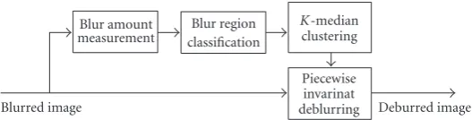
Recently, the piecewise shift invariant model has been applied to the LSV image restoration [7]. The image is firstly segmented into the blurred and unblurred regions, and the RL algorithm is performed only to the blurred region by using the estimated PSF. However, this technique is applicable to the image of a single blurred object and unblurred background. In order to apply the proposed LSI deblurring technique to more general LSV image deblurring problem, we develop a piecewise shift invariant deblurring algorithm as shown in Figure 8. In our method, image segmentation method is employed to divide the image into different regions that can be considered as the LSI model. To segment the image, the amount of blur is calculated by the no-reference blur metric [12]. Since motion blur spreads the edges of the image, the length of the spread edge is relatively proportional to the amount of blur. After applying the edge operator to the blurred image, the length of spread edge is measured at every edge pixel. Pixels belonging to the edges and their spread, that is, the edgewidth mask inSection 3, are considered to be blurred pixels. Then,K-median clustering [16] with the proposed distance metric is applied to divide the blurred pixels into different regions. Within the blurred pixels, three distances including the distance of blur amount Db, the distance of pixel valueDp, and the distance of pixel position Dd are defined to measure the similarity between two pixels,x1andx2, as follows:
Db(x1,x2)= |B(x1)−B(x2)|,
Dp(x1,x2)= |I(x1)−I(x2)|,
Dd(x1,x2)= x1−x22,
(15)
whereB,I, and · 2represent the estimated blur amount, the pixel value, and the L-2 norm, respectively. Note that the blur amount of each pixel represents the edgewidth [12] as explained in theSection 3.
A scaled distance,Ds(x1,x2), used forK-median cluster-ing, is defined as a weighted sum of the three distances:
Ds(x1,x2)=α1Db(x1,x2) +α2Dp(x1,x2) +α3Dd(x1,x2). (16)
Blurred image Blur amount measurement Blur region classification K-median clustering Piecewise invarinat
deblurring Deburred image Figure8: Shift variant deblurring process.
6. Experimental Results
6.1. LSI PSF Estimation Accuracy. In all of the experiments of the proposed PSF estimation, we locally spread the PSF using the four directional spreading operators defined inSection 2. In order to evaluate the performance of the proposed LSI PSF estimation, the test images,Lena,Airplane,Barbara, and
Peppers, were degraded by applying the sample PSFs shown inFigure 9. Each sample PSF,hs, was obtained by combining the uniform motion blur and the random blur as follows:
hs=h0∗hr, (17)
where h0 represents the uniform motion blur defined in (11). In order to introduce a randomness of the PSF, the random blur,hr, is combined toh0. Here,hr is in a form of N×Nmatrix whose coefficients are randomly chosen within a range of [0, 1) while satisfying (10).
Then, the degraded images are used as initial estimates of iterative PSF estimation process. For the initialization of the PSF, the length and the direction of the linear motion blur are estimated from the blurred image [7].Figure 10shows PSF estimation results onAirplaneimage blurred by the PSF in Figure 9(a). As can be seen from Figures 10(b), 10(c), and10(d), the shape and the size of the PSF are efficiently estimated.
To evaluate quantitatively the performance of the pro-posed PSF estimation method, the quality of deblurred images of the proposed method and the conventional method is compared. Since we have original images, the ISNR [11] can be used for the quantitative measurement of the quality of the deblurred image which is defined as
ISNR=10 log
⎧ ⎪ ⎨ ⎪ ⎩
(x,y)∈Sf
f(x,y)−g(x,y)2
(x,y)∈Sf
f(x,y)−fx,y2
⎫ ⎪ ⎬ ⎪
⎭, (18)
where f, g, f, and Sf denote the original image, the blurred image, the deblurred image, and the image support, respectively. Since the ISNR increases as the quality improves, the best deblurred image is the one that has the highest ISNR.
Table 1 shows the ISNR comparison results. All of the deblurred results were obtained by 10 iterations of the accelerated RL algorithm. Since the proposed algorithm estimates the PSF from the image itself, the ISNR results were dependent on the image features. However, the results showed that the overall ISNRs of the proposed method approached those of the ideal case where the original PSF was used. From these ISNR results, we can conclude that
the proposed algorithm can estimate the PSF with a high accuracy.
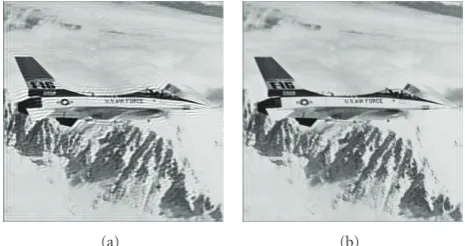
In Figure 11, the normalized cost function obtained by using Figure 9(a) and Airplane image is illustrated, where λ is chosen as 0.5. As explained in Section 4, if a certain directional spreading reduces the cost function, the test of that direction is repeated. Otherwise, the remaining directions are tested. The proposed algorithm terminates when all the spreading operators are used. Here, the final PSF shown inFigure 10(c)was achieved after 40 updates of the PSF. Then, the accelerated RL deconvolution is applied with the estimated PSF. The original and its corresponding blurred images are given in Figures 4(a) and 4(b), and the restoration result inFigure 12shows that the proposed method effectively restores the image without excessive restoration artifacts.
Next, we examined the performance of the proposed LSI image restoration algorithm on a real-blurred image. The test image shown in Figure 13(a) was taken with a high-end DSLR with enough exposure time for capturing the image without excessive noise. Since the image was captured with the global horizontal motion of the camera, the blur inFigure 13(a)was assumed shift invariant. The restoration result shown inFigure 13(b)demonstrates that the proposed algorithm is applicable to the real-blurred image when the PSF can be considered as the LSI.
0 0.05 0.1
P
o
int
spr
ead
function
−4
0
4
X −4
0 4
Y
(a)
0 0.05 0.1
P
o
int
spr
ead
function
−6 −3
0 3
6
X −4
0 4
Y
(b)
0 0.03 0.06
P
o
int
spr
ead
function
−4
0
4
X −5
0 5
Y
(c)
0 0.02 0.04
P
o
int
spr
ead
function
−2
0
2
X −8
−4 0 4
8
Y
(d)
Figure9: Four sample PSFs with the following parameters. (a)L=9,θ=135◦, andN =3. (b)L=11,θ=30◦, andN =3. (c)L=7,
θ=60◦, andN=5. (d)L=13,θ=90◦, andN=5.
Table1: ISNR(dB) comparison of deblurred results.
PSF Image
Original Estimated Lena Airplane Barbara Peppers
PSF inFigure 9(a)
by [7] 1.21 0.55 1.65 1.32
by the proposed method 3.19 2.16 2.72 3.11
PSF inFigure 9(a) 3.57 2.82 3.05 4.88
PSF inFigure 9(b)
by [7] 1.89 2.93 3.27 3.18
by the proposed method 3.36 3.28 3.71 4.55
PSF inFigure 9(b) 4.19 3.62 4.12 5.02
PSF inFigure 9(c)
by [7] 0.37 0.72 0.58 0.42
by the proposed method 2.45 3.00 2.83 2.94
PSF inFigure 9(c) 2.79 3.29 3.01 4.12
PSF inFigure 9(d)
by [7] 0.27 0.61 0.83 1.35
by the proposed method 1.89 2.52 1.40 2.79
PSF inFigure 9(d) 2.35 2.69 2.14 3.36
and nonblurred regions, the quality of the deblurred image shown in Figure 14(e) is not satisfactory. The proposed segmentation-based piecewise invariant approach visually produces a better result as shown inFigure 14(f). Since the original image is given in this simulation, the ISNR can
0 0.05 0.1
P
o
int
spr
ead
function
−3
0
3
X −3
0 3
Y
(a)
0 0.05 0.1
P
o
int
spr
ead
function
−6 −3
0 3
6
X −6
−3 0
3 6
Y
(b)
0 0.05 0.1
P
o
int
spr
ead
function
−5
0
5
X −5
0 5
Y
(c)
−0.04
−0.02
−50 0.02 0.04
P
o
int
spr
ead
function
0 5
X
−5 0
5
Y
(d)
Figure10: PSF estimation results usingAirplaneimage and the sample PSF inFigure 9(a). (a) Initial PSF estimated by [7]. (b) Estimated
PSF after 20 updates. (c) Estimated PSF after 40 updates. (d) Estimation error between Figures9(a)and10(c).
Table2: Quantitative evaluation of deblurred results in real blurred images.
Image Algorithm PMOS
Miniature
[7]’s 77.01
Proposed K=5 78.37
K=10 78.31
K=20 82.10
K=30 82.22
Doll
[7]’s 76.34
Proposed K=5 78.42
K=10 78.88
K=20 79.87
K=30 80.59
For the sake of implementation on image deconvolution, a rectangular segment is preferred instead of an arbitrary shaped segment. Therefore, we construct a rectangular block of minimum size for each segment. For each pixel of the segment, the minimum and the maximum pixel coordinates of the horizontal axis and the vertical axis are used to obtain the rectangular block as shown in Figure 14(d). Then, the
0.92 0.94 0.96 0.98 1
Co
st
fu
n
ct
ion
10 20 30 40
Number of updates
Figure11: Cost function result onAirplaneimage blurred by the
PSF inFigure 10(a).
(a) (b)
Figure12: Restoration results of numerically blurred image where the PSF is estimated after 40 updates. (a) Restored image by using
the conventional algorithm [7]. (b) Restored image by using the
proposed.
the magnified regions of restoration results in Figures14(g)–
14(l), we can see that the proposed method outperforms the conventional method.
Next, we applied the proposed algorithm to the real blurred images also captured with a high-end DSLR. The
Miniatureimage shown inFigure 15(a)was taken under 150 lux with shutter speed of 1/20 (sec) and blurred by a camera shake during the exposure time. In this high-resolution image whose spatial resolution is 1280 by 1024, the PSF of the whole image cannot be assumed to be shift invariant. Since the number of segments is not known in advance, a relatively large number should be used. We set K as 20 in this experiment. Other experimental parametersα1,α2, and α3are set as 3, 2, and 1, respectively.Figure 15(b)shows the segmentation result of the proposed method. In this figure, different luminance indicates a different segment. Since smooth regions are not affected by blur, those regions whose luminance is zero are not included in the segmentation. Each segment is deblurred by the aforementioned technique, and final result is compared with the result of the conventional piecewise shift-invariant approach [7]. From the magnified
(a) (b)
Figure13: Restoration results of real-blurred image. (a) Test image. (b) Restoration result of the proposed method, where the final PSF is achieved after 27 updates.
region of each result shown in Figures15(c)–15(f), we can subjectively compare the performances of the results.
Figure 16 shows another experimental result with a different experimental condition. TheDollimage shown in
Figure 16(a)was taken under 180 lux with shutter speed of 1/20 (sec) and blurred by a horizontal motion of camera during the exposure time. In the experiment, the same experimental parameters used inFigure 15were maintained. As can be seen inFigure 16(b), blurred regions are separated, so each segment can be deblurred by its own estimated PSF. From the magnified region of each result shown in Figures
16(c)–16(f), we can also subjectively see the superiority of the proposed method. Note that even though the image is simply blurred by a global horizontal motion of the camera, more improved quality can be achieved by the proposed PSF estimation and piecewise LSI restoration.
We also quantitatively measured the performance of the proposed algorithm for the real blurred images. Since the original image is not given in this general restoration prob-lem, we examined a no-reference (NR) quality assessment (QA) [18] to compare the performances of the proposed and conventional algorithms. In [18], natural scene statistics are blindly measured and the quality is expressed by the predicted mean opinion scores (PMOSs), where the higher PMOS represents the better quality. The PMOS results in
Table 2demonstrate that the proposed algorithm quantita-tively performs better than the conventional algorithm.
To examine the effect of the number of segment, the results with various K are also given in Table 2. As can be seen, the performance is gradually improved asK increases untilK reaches a sufficient number, which is 20. Note that Kis dependent on the type of image blur. ForFigure 16(a), which is blurred by a horizontal camera motion, a relatively lowKprovides comparable result with the results with high K. However, for an image blurred by a camera shake such asFigure 15(a), a highKis preferred to provide a sufficient quality of the resultant image.
7. Conclusion
(a) (b)
(c) (d)
(e) (f)
(g) (j)
(h) (i) (k) (l)
Figure14: Restoration results on simulated shift variant blur images [7]. (a) Original image. (b) Blurred image. (c) Segmentation result. (d)
Segmentation result with rectangular block. (e) Restoration result of [6]. (f) Restoration results of the proposed method. (g)–(i) Magnified
(a) (b)
(c) (d) (e) (f)
Figure15: Comparison of restoration results onMiniatureimage. (a) Blurred image. (b) Segmentation result. (c)-(d) Magnified region of
the deblurred image obtained by [7]. (e)-(f) Magnified region of the deblurred image obtained by the proposed algorithm.
(a) (b)
(c) (d) (e) (f)
Figure16: Comparison of restoration results onDollimage. (a) Blurred image. (b) Segmentation result. (c)-(d) Magnified region of the
deblurred image obtained by [7]. (e)-(f) Magnified region of the deblurred image obtained by the proposed algorithm.
directional spreading operator is applied only when the update of the PSF reduces the cost function, the amount of blur can be decreased without excessive restoration artifacts in the restored image. Piecewise shift invariant approach with the proposed image segmentation method is applied to deal with the LSV PSF. Throughout the experiments, the proposed PSF estimation algorithm can efficiently estimate the PSF when the parametric model of the PSF is inaccurate.
The generalization of the LSI algorithm to the LSV shows relatively better performance in comparison with the con-ventional algorithm.
methods need to be considered. In the future, we plan to extend our approach to remove motion blur of fast moving objects using video sequences.
Acknowledgment
This research was supported by Seoul Future Contents Convergence (SFCC) Cluster established by Seoul R&BD Program.
References
[1] A. K. Katsaggelos, “Iterative image restoration algorithms,” Optical Engineering, vol. 28, no. 7, pp. 735–748, 1989. [2] D. B. Gennery, “Determination of optical transfer function by
inspection of frequency-domain plot,”The Optical Society of
America, vol. 63, pp. 1571–1577, 1973.
[3] R. L. Lagendijk, J. Biemond, and D. E. Boekee, “Identification and restoration of noisy blurred images using the
expectation-maximization algorithm,” IEEE Transactions on Acoustics,
Speech, and Signal Processing, vol. 38, pp. 1180–1191, 1990. [4] G. Pavlovi´c and A. M. Tekalp, “Maximum likelyhood
paramet-ric blur identification based on a continuous spatial domain
model,”IEEE Transactions on Image Processing, vol. 1, pp. 496–
504, 1992.
[5] D. L. Tull and A. K. Katsaggelos, “Iterative restoration of
fast-moving objects in dynamic image sequences,” Optical
Engineering, vol. 35, no. 12, pp. 3460–3469, 1992.
[6] Y.-L. You and M. Kaveh, “A regularization approach to joint
blur identification and image restoration,”IEEE Transactions
on Image Processing, vol. 5, pp. 416–428, 1996.
[7] A. Levin, “Blind motion deblurring using image statistics,” inAdvances in Neural Information Processing Systems (NIPS), 2006.
[8] J. Bardsley, S. Jefferies, J. Nagy, and R. Plemmons, “Blind
iterative restoration of images with spatially-varying blur,” Optics Express, vol. 14, pp. 1767–1782, 2006.
[9] L. Bar, N. Sochen, and N. Kiryati, “Variational pairing of image
segmentation and blind restoration,” inProceedings of the 8th
European Conference on Computer Vision (ECCV ’04), Prague, Czech Republic, May 2004.
[10] P. A. Jansson,Deconvolution of Image and Spectra, Academic
Press, San Diego, Calif, USA, 1997.
[11] K. L. May, T. Stathaki, and A. K. Katsaggelos, “Spatially
adaptive intensity bounds for image restoration,”EURASIP
Journal on Applied Signal Processing, vol. 2003, no. 12, pp. 1167–1180, 2003.
[12] P. Marziliano, F. Dufaux, S. Winkler, and T. Ebrahimi, “A
no-reference perceptual blur metric,” in Proceedings of the
International Conference on Image Processing (ICIP ’02), vol. 3, pp. 57–60, Rochester, NY, USA, September 2002.
[13] J. Canny, “A computational approach to edge detection,”IEEE
Transactions on Pattern Analysis and Machine Intelligence, vol. 8, pp. 679–698, 1986.
[14] D. S. C. Biggs and M. Andrews, “Acceleration of iterative image
restoration algorithms,”Applied Optics, vol. 36, no. 8, 1997.
[15] M. K. Ozkan, A. M. Tekalp, and M. I. Sezan,
“POCS-based restoration of space-varying blurred images,” IEEE
Transactions on Image Processing, vol. 3, no. 4, pp. 450–454, 1994.
[16] C. W. Therrien,Decision Estimation and Classification, IEEE
Wireless Communications, John Wiley & Sons, New York, NY, USA, 1989.
[17] R. C. Gonzalez and R. E. Woods, Digital Image Processing,
Prentice-Hall, Upper Saddle River, NJ, USA, 2002.