Volume 2006, Article ID 84614, Pages1–29 DOI 10.1155/ASP/2006/84614
Low-Cost Super-Resolution Algorithms Implementation over
a HW/SW Video Compression Platform
Gustavo M. Callic ´o,1Rafael Peset Llopis,2Sebastian L ´opez,1Jos ´e Fco. L ´opez,1Antonio N ´u ˜nez,1 Ramanathan Sethuraman,3and Roberto Sarmiento1
1The University of Las Palmas de Gran Canaria, Institute for Applied Microelectronics (IUMA), Tafira Baja, 35017, Spain 2Philips Consumer Electronics, SFJ-6, P.O. Box 80002, 5600 JB, The Netherlands
3Philips Research Laboratories, WDC 3.33, Professor Holstlaan 4, 5656 AA Eindhoven, The Netherlands
Received 1 December 2004; Revised 5 July 2005; Accepted 8 July 2005
Two approaches are presented in this paper to improve the quality of digital images over the sensor resolution using super-resolution techniques: iterative super-super-resolution (ISR) and noniterative super-super-resolution (NISR) algorithms. The results show important improvements in the image quality, assuming that sufficient sample data and a reasonable amount of aliasing are avail-able at the input images. These super-resolution algorithms have been implemented over a codesign video compression platform developed by Philips Research, performing minimal changes on the overall hardware architecture. In this way, a novel and feasible low-cost implementation has been obtained by using the resources encountered in a generic hybrid video encoder. Although a specific video codec platform has been used, the methodology presented in this paper is easily extendable to any other video en-coder architectures. Finally a comparison in terms of memory, computational load, and image quality for both algorithms, as well as some general statements about the final impact of the sampling process on the quality of the super-resolved (SR) image, are also presented.
Copyright © 2006 Hindawi Publishing Corporation. All rights reserved.
1. INTRODUCTION
Here are two straightforward ways to increase sensor resolu-tion. The first one is based on increasing the number of light sensors and therefore the area of the overall sensor, result-ing in an important cost increase. The second one is focused on preserving the overall sensor area by decreasing the size of the light sensors. Although this size reduction increases the number of light sensors, the size of the active pixel area where the light integration is performed decreases. As fewer amounts of light reach the sensor it will be more sensitive to the shot noise. However, it has been estimated that the min-imum photo-sensors size is around 50μm2[1], a limit that has already been reached by the CCD technology. A smart so-lution to this problem is to increase the resoso-lution using algo-rithms such as the super-resolution (SR) ones, wherein high-resolution images are obtained using low-high-resolution sensors at lower costs. Super-resolution can be defined as a technique that estimates a high-resolution sequence by using multiple observations of the scene using lower-resolution sequences. In order to obtain significant improvements in the result-ing SR image, some amount of aliasresult-ing in the input low-resolution images must be provided. In other words, if all the high-frequency information has been removed from the
input images (for instance by using lenses with optical low-pass filter effect), it will be impossible to recover the edge de-tails contained in the high frequencies. Some of the most im-portant applications of SR are as follows.
(i) Still-image improvement [1–4], where several images from the same scene are obtained and used to con-struct a higher-resolution image.
(ii) Analog video frame improvement [5,6]. Due to the low quality of analog video frames, they are not nor-mally suitable to directly perform a printed-copy dig-ital photography. The quality of the image is in-creased using several consecutive frames combined in a higher-resolution image by using SR algorithms. (iii) Surveillance systems [7], where SR is used to increase
the quality in video surveillance systems, using such recorded sequences as forensic digital video, and even to be admitted as evidence in the courts of law. SR im-proves night vision systems when images have been ac-quired with infrared sensors [8] and helps in the face recognition process for security purposes [9].
(v) Medical image acquisition [11]. Many medical types of equipment as the computer-aided tomography (CAT), the magnetic resonance images (MRI), or the echogra-phy or ultrasound images allow the acquisition of sev-eral images, which can be combined in order to obtain a higher-resolution image.
(vi) Improvement of images from compressed video [12– 15]. For example, in [16] the images high-frequency information recovery, lost in the compression process, is addressed. The missing data are incorporated from transform-domain quantization information obtained from the compressed video bit stream. An excellent survey of SR algorithms from compressed video can be found in [17].
(vii) Improvement of radar images [18,19]. In this case SR allows a clearer observation of details sometimes crit-ical for air or maritime security [20] or even for land observations [21–24].
(viii) Quality improvement of images obtained from the outer space. An example is exposed in [4] with images taken by the Viking satellite.
(ix) Image-based rendering (IBR) of 3D objects uses cam-eras to obtain rich models directly from the real-world data [26]. SR is used to produce high-resolution scene texture from an omnidirectional image sequence [26,27].
This paper addresses low-cost solutions for the imple-mentation of SR algorithms on SOC (system-on-chip) plat-forms in order to achieve high-quality image improvements. Low-cost constrains are accomplished by reusing a video coder, rather than developing a specific hardware. This en-coder can be used either in the compression mode or in the SR mode as an added value to the encoder. Due to this rea-son, SR is used in the video encoder as a smart way to per-form image zooming of regions of interest (ROI) without us-ing mechanical parts to move the lenses, thus savus-ing power dissipation. It is important to remark that although the SR algorithms presented in this paper have been implemented on an encoder architecture developed by Philips Research, the same SR algorithms can be easily adapted to other hybrid video encoder platforms.
The SR approaches that will be depicted consist of gather-ing information from a set of images in the spatial-temporal domain in order to integrate all the information (when pos-sible) in a new quality-improved super-resolved image. This set is composed of several images, where small spatial shifts have been applied from one image to the other. This is achieved by recording a video sequence at high frame rates with a hand-held camera.
The reconstruction problem using SR can be defined as the objective of reconstructing an image or video sequence with a higher quality or resolution from a finite set of lower-resolution images taken from the same scene [28, 29], as shown inFigure 1. This set of low-resolution images must be obtained under different capturing conditions of the image, from different spatial positions, and/or from different cam-eras. This reconstruction problem is an aspect of the most general problem of sensor fusion.
Pixels adjustment
Super-resolution
Low-resolution observed images
Images acquisition Reconstruction
process
Reconstructed image Original image
Figure 1: Model of the reconstruction process using
super-res-olution.
The rest of the paper is organized as follows. Firstly, the most important publications directly related to this work are reviewed, followed by a brief description of the hybrid video compression architecture where the developed SR algorithms have been mapped. In the second section the bases of the ISR algorithms are established while inSection 3the mod-ifications needed to be implemented onto the video encoder are described. InSection 4the experimental setup to eval-uate the quality of the iterative and noniterative algorithms is presented, and based on it, a set of experiments is devel-oped inSection 5in order to assess the correct behavior of the ISR algorithm, showing as a result an important increase in the super-resolved output images. As far as an iterative be-havior seriously jeopardizes a real-time implementation, in Section 6a novel SR algorithm is described, where the pre-vious iterative feature has been removed. In the same sec-tion, the adjustments carried out in the architecture in or-der to obtain a feasible implementation are explained, while Section 7shows the results achieved with this noniterative al-gorithm. In Section 8the advantages and drawbacks of the described ISR and NISR algorithms are compared and finally, inSection 9, the most remarkable results of this work are pre-sented.
1.1. Super-resolution algorithms
problem of registration and restoration (the registration im-plies estimating the relative shifts among the observations and the restoration implies the estimation of samples on a uniform grid with a higher sampling rate). The restora-tion stage is actually an interpolarestora-tion problem dealing with nonuniform sampling. From the Huang and Tsay proposal until the present days, several research groups have devel-oped different algorithms for this task of reconstruction, ob-tained from different strategies or analyses of the problem.
The great advances experimented by computer technol-ogy in the last years have led to a renewed and growing inter-est in the theory of image rinter-estoration. The main approaches are based on nontraditional treatment of the classical restora-tion problem, oriented towards new restorarestora-tion problems of second generation, and the use of algorithms that are more complex and exhibit a higher computational cost. Based on the resulting image, these new second-generation algo-rithms can be classified into problems of an image restora-tion [30,33–36], restoration of an image sequence [37–40], and reconstruction of an image improved with SR [41–47]. This paper is based on the last mentioned approach, both for the reconstruction of static image as for the reconstruction of image sequences with SR improvements.
The classical theory of image restoration from blurred images and with noise has caught the attention of many re-searchers over the last three decades. In the scientific liter-ature, several algorithms have been proposed for this clas-sical problem and for the problems related to it, contribut-ing to the construction of a unified theory that comprises many of the existing restoration methods [48]. In the im-age restoration theory, mainly three different approaches ex-ist that are widely used in order to obtain reliable restoration algorithms: maximum likelihood estimators (MLE) [48–50], maximum a posteriori (MAP) probability [48–51], and the projection onto convex sets (POCS) [52].
An alternative classification [53] based on the process-ing approach can be made, where the work on SR can be di-vided into two main categories: reconstruction-based meth-ods [46,54] and learning-based methods [55–57]. The theo-retical foundations for reconstruction methods are nonuni-form sampling theorems, while learning-based methods em-ploy generative models that are learned from samples. The goal of the former is to reconstruct the original (supersam-pled) signal while that of the latter is to create the signal based on learned generative models. In contrast with recon-struction methods, learning-based SR methods assume that corresponding low-resolution and high-resolution training image pairs are available. The majority of SR algorithms be-long to the signal reconstruction paradigm that formulates the problem as a signal reconstruction problem from multi-ple sammulti-ples. Among this category are frequency-based meth-ods, Bayesian methmeth-ods, back-projection (BP) methmeth-ods, pro-jection onto convex set (POCS) methods, and hybrid meth-ods. From this second classification, this paper is based on the reconstruction-based methods, as it seeks to reconstruct the original image without making any assumption about the generative models and assuming that only the low-resolution images are available.
The problem of a specific image reconstruction from a set of lower-quality images with some relative movement among them is known as the static SR problem. On the other side is the dynamic SR problem, where the objective is to obtain a higher-quality sequence from another lower-resolution se-quence, seeking that both sequences have the same length. These two problems also can be denominated as the SR prob-lem for static images and the SR probprob-lem for video, respec-tively [58]. The work presented in this paper only deals with static SR as the output sequences do not have the same length of the input low-resolution sequences.
Most of the proposed methods mentioned above lack fea-sible implementations, leaving aside the more suitable pro-cess architectures and the required performances in terms of speed, precision, or costs. Although some important optimi-sation effort has been done [59], most of the previous SR approaches demand a huge amount of computation, and for this reason, in general they are not suitable for real-time ap-plications. Until now, none of them have been implemented over a feasible hardware architecture. This paper addressed this fact and offers a low-cost solution. The ISR algorithm exposed in this paper is a modified version of [60], adapted to be executed inside a real video encoder, that is, restricting the operators needed to those that can be found in such kind of platforms. New operator blocks to perform the SR process have been implemented inside the existing coprocessors in order to minimize the impact on the overall architecture, as will be demonstrated in the next sections.
1.2. The hybrid video encoder platform
All the algorithms described in this paper have been imple-mented in an architecture developed by Philips Research. This architecture is shown in Figure 2. The software tasks are executed on an ARM processor and the hardware tasks are executed on the very long instruction word (VLIW) pro-cessors (namely, pixel processor, motion estimator processor, texture processor, and stream processor). The pixel processor (PP) communicates with the pixel domain (image sensor or display) and performs input lines to macroblock (MB) con-versions. The motion estimator processor (MEP) evaluates a set of candidate vectors received from the software part and selects the best vector for full-, half-, and quarter-pixel refinements. The output of the MEP consists of motion vectors, sum-of-absolute-difference (SAD) values, and tex-ture metrics. This information is processed by the general-purpose embedded microprocessor ARM to determine the encoding approach for the current MB.
The texture processor (TP) performs the MB encoding and stores the decoded MBs in the loop memory. The output of the TP consists of variable-length encode (VLE) codes for the discrete cosine transform (DCT) coefficients of the cur-rent MB. Finally, the stream processor (SP) packs the VLE-coded coefficients and headers generated by the TP and the ARM processor, respectively.
through a bridge. Images that will be processed by the ISR and NISR algorithms come from the data bus.
2. ITERATIVE SUPER-RESOLUTION ALGORITHMS
In this section the bases for the formation of super-resolved images starting from lower-resolution images are exposed. For this purpose, if f( ˘x, ˘y,t) represents the low-resolution input image, and it is assumed that all the input subsystem effects (lenses filtering, chromatic irregularities, sample dis-tortions, information loss due to format conversions, system blur, etc.) are included inh(x,y), the input to the iterative algorithm is obtained by the two-dimensional convolution expressed as
g(x,y,t)= f( ˘x, ˘y,t)∗ ∗h(x,y), (1)
where a lineal behavior for all the distortion effects has been supposed. Denoting SR( ˘x, ˘y) as the SR algorithm, the image obtainedS( ˘x, ˘y,t) after applying this algorithm is as follows:
S( ˘x, ˘y,t)=g(x,y,t)∗ ∗SR( ˘x, ˘y), (2)
where (x,y) are the spatial coordinates in the low-resolution grid, ( ˘x, ˘y) are the spatial coordinates in the SR grid, and “t” represents the time when the image was acquired. These rela-tionships are summarized inFigure 3(a)concerning the real system and are simplified inFigure 3(b).
The algorithm characterized by SR( ˘x, ˘y) starts supposing that a number of “p” low-resolution images of sizeN×M
pixels are available asg(x,y,ti), where “ti” denotes the
sam-pling time of the image. The possibility of increasing the size of the output image in every direction on a predefined amount, called scale factor (SF), has been considered. There-fore, the output image has a size of SF·N×SF·M. As the algorithm refers to only the last “p” images, from now on the index “l”, defined asl=imodp, will be used to refer to the images inside the algorithm’s temporal window (Figure 4). Thus, the memory imagegl(x,y) is linked tog(x,y,ti) as fol-lows:
g
l(x,y)=g
x,y,ti
l =imodp. (3)
In this way, ¯gl(x,y) represents the average input image, as given in (4), which is used as the first reference in the fol-lowing steps:
¯
g(x,y)=1
p p−1
l=0
1
N·M·
N−1
i=0
M−1
j=0
g
l(i,j)
, ∀x,y. (4)
The average error for the first iteration is then obtained by computing the differences between this average image and each of the input images, as shown in (5), where the super-script denotes the iteration number (first iteration in this case):
el(x,y)(1)=g
l(x,y)−g¯(x,y), l=0,. . ., (p−1). (5)
This error must be transformed to high-resolution coor-dinates by means of a nearest-neighbor replication interpola-tor (6) of size SF. It is essential to use this type of interpolainterpola-tor as it will preserve the necessary aliasing required for the SR process. InSection 5, the undesirable effect of using a bilinear interpolator will be shown:
el( ˘x, ˘y)(1)=upsampleel(x,y)(1), SF, l=0,. . ., (p−1). (6)
Once the upsample process has been completed, the error must be adjusted to the reference frame by shifting the error imageΔδl(x,y)(1)(fr2ref)andΔλl(x,y)(1)(fr2ref)amounts in the hor-izontal and vertical coordinates, respectively, where (fr2ref) means that the displacement is computed from every frame to the reference and (ref2fr) means that the displacement is computed from the reference to every frame. In principle, these displacements are applied to every pixel individually, depending upon the employed motion estimation technique. As far as these displacements will be used in high resolution, they must be properly scaled by SF as shown:
Δδl( ˘x, ˘y)=SF·Δδl(x,y),
Δλl( ˘x, ˘y)=SF·Δλl(x,y). (7)
When all the errors have been adjusted to the reference, they are averaged, taking this average as the first update of the SR image, as shown:
S0( ˘x, ˘y)(1)
= 1p ·
p−1
l=0
el
˘
x+Δδl( ˘x, ˘y)(fr2ref)(1) , ˘y+Δλl( ˘x, ˘y) (1) (fr2ref)
(1)
.
(8)
Equation (8) reflects the result of the first iteration, where
S0( ˘x, ˘y)(1)is the first version of the SR image, corresponding tot=t0, being upgraded with each iteration. Thenth iter-ation begins obtaining a low-resolution version of this im-age by decimation, followed by the computation of the dis-placements between every one of these inputs images and this decimated image and vice versa, that is, between the deci-mated image and the input images. In this way, the displace-ments of thenth iteration will be available:Δδl(x,y)((fr2ref)n) ,
Δλl(x,y)(fr2ref)(n) ,Δδl(x,y)((ref2fr)n) , andΔλl(x,y)((ref2fr)n) . The low-resolution version of the image obtained in high low-resolution is given by (9).
S0(x,y)(n)=downsampleS0( ˘x, ˘y)(n−1), SF. (9)
The downsample operation is defined in the following where only pixels in certain coordinates given by SF are kept:
g(x,y)=downsamplef( ˘x, ˘y), SF,
g(x,y)= f(SF·x, SF·y). (10)
Pixel
processor Bridge
Motion estimator processor
Texture processor
Data-bus Stream processor Ctrl-bus
Image memory
BCU BCU Outside
communications ARM
ARM memory
Figure2: Architecture for the multistandard video/image codec developed in Philips Research.
G R G R
B G B G
G R G R
B G B G
G R G R
f(x, y, t)
h(x, y)
Lenses Sensor DSP
RGB g(x, y, t)
YCbCr 4 : 2 : 0
S( ˘x,y, t˘ ) SR( ˘x,y˘)
Hybrid video compressor
Input subsystem Super-resolution subsystem CP CP CP
μP RAM
(a)
f(x, y, t) h(x, y) g(x, y, t) SR( ˘x,y˘) S( ˘x,y, t˘ ) (b)
Figure3: (a) Scheme of the real overall system and (b) the simplified model, together with the used terminology.
I=0 I=1 I=2 I=3 I=0 I=1
g¼
0(x, y, t) g
¼
1(x, y, t) g
¼
2(x, y, t) g
¼
3(x, y, t) g
¼
0(x, y, t) g
¼
1(x, y, t)
i=0 i=1 i=2 i=3 i=4 i=5
g(x, y, t0) g(x, y, t1) g(x, y, t2) g(x, y, t3) g(x, y, t4) g(x, y, t5)
t0 t1 t2 t3 t4 t5
t
displacementsΔδl(x,y)(ref2fr)(n) andΔλl(x,y) (n)
(ref2fr), converting them to low-resolution and getting the error with respect to every input image, as shown:
el(x,y)(n)=g
l(x,y)
−S0
x+Δδl(x,y)(ref2fr)(n) , y+Δλl(x,y) (n) ref2fr
(n) ,
l=0,. . ., (p−1). (11)
This low-resolution error image must be transformed again into a high-resolution one through interpolation and compensate for its motion again towards the reference. The average of these “p” errors constitutes thenth incremental update of the high-resolution image, as shown:
S0( ˘x, ˘y)(n)=S0( ˘x, ˘y)(n−1)+ 1
p
·
p−1
l=0
el
˘
x+Δδl( ˘x, ˘y)(fr2ref)(n) , ˘y+Δλl( ˘x, ˘y) (n) (fr2ref)
(n)
.
(12)
The convergence is reached when the changes in the av-erage error are negligible, that is, when the variance of the average error is below a certain threshold determined in an empirical procedure.
Once the SR image is obtained for timet0with the first “p” images, the process must be repeated with the next “p” images to obtain the next SR image using a previously es-tablished number of iterations or iterating until convergence is reached. To obtain an SR image implies the use of “p” low-resolution images, hence, at instant ti, the SR image
k=integer(i/p) is generated. In such case, (11) must be gen-eralized to
Sk( ˘x, ˘y)(n)=Sk( ˘x, ˘y)(n−1)+ 1
p
·
p−1
l=0
elx˘+Δδl( ˘x, ˘y)((fr2ref)n) , ˘y+Δλl( ˘x, ˘y)(fr2ref)(n) (n).
(13)
This equation shows the SR image at instantkas a com-bination of “p” low-resolution images after “n” iterations.
3. MODIFICATIONS FOR THE IMPLEMENTATION ON A VIDEO ENCODER
3.1. Algorithm modifications
The modifications to the ISR algorithm previously presented are intended to adapt the algorithm in terms of basic actions that are easily implemented on a video encoder, as will be detailed in this section. First of all, instead of starting with an average image as indicated in (4) several experiments carried out have demonstrated that it is faster and easier to start with an upsampled version of the first low-resolution input image. Therefore, the final SR image will be aligned with the first image, whose motion is well known.
The straightforward way in a video encoder to determine the displacements between pictures is by using the motion estimator, which is normally used to code interpictures of typeP orBin many video coding standards such as MPEG or H.26x. Furthermore, as the displacements computation is one of the most sensitive steps in the ISR algorithm, as well as in all the SR algorithms found in the literature, it has been decided to use a motion estimator with a quarter-pixel pre-cision for this task. Consequently, the motion compensator must be also prepared to work with the same precision in order to displace a picture. The main drawback is that the ISR algorithm presented is intended to work on a pixel ba-sis, while the motion estimator and compensator of the com-pressor work on a block basis. This mismatch produces qual-ity degradation when the motion does not match the block sizes, that is, when the object is smaller that the block size or when more than one moving object exist inside the block.
Another problem found in order to map the ISR algo-rithm into the video encoder architecture is derived from the fact that the addition of twoN-bit numbers produces an
N+ 1 bit number. Every pixel inside the encoder architecture is represented as an 8- bit number. Inside the co-processors, the pixel values are processed performing several additions, and for this reason the precision of the adders has been in-creased. On the other hand the results must be stored in an 8- bit image memory. For video compression, this precision loss is not a significant problem, but when reusing the same architecture for general image processing, the limitation of storing the intermediate results in 8- bit memories becomes an important issue. Due to that, the following solutions have been adopted [61]:
(i) implement as many arithmetic operations as possible inside the coprocessor, increasing the precision; (ii) rearrange the arithmetic operations in such a way
that, when storing the intermediate results, these are bounded, as close as possible, to 8- bit numbers.
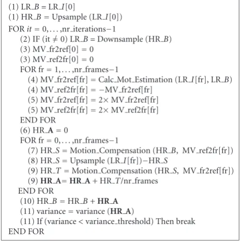
(1) LRB=LRI[0]
(1) HRB=Upsample (LRI[0]) FORit=0,. . .,nr iterations−1
(2) IF (it=0) LRB=Downsample (HRB) (3) MV fr2ref[0]=0
(3) MV ref2fr[0]=0 FOR fr=1,. . .,nr frames−1
(4) MV fr2ref[fr]=Calc Mot Estimation (LRI[fr], LRB) (4) MV ref2fr[fr]= −MV fr2ref[fr]
(5) MV fr2ref[fr]=2×MV fr2ref[fr] (5) MV ref2fr[fr]=2×MV ref2fr[fr] END FOR
(6) HRA=0
FOR fr=0,. . .,nr frames−1
(7) HRS=Motion Compensation (HRB, MV ref2fr[fr])
(8) HRS=Upsample (LRI[fr])−HRS
(9) HRT=Motion Compensation (HRS, MV fr2ref[fr])
(9)HR A=HR A+ HRT/nr frames
END FOR
(10) HRB=HRB+HR A
(11) variance=variance (HR A)
(11) If (variance<variance threshold) Then break END FOR
Algorithm1: Pseudocode of the ISR algorithm implemented on the video encoder.
(1) Initially, the first low-resolution image is stored in LR B, used as the low-resolution version of the super-resolved image that will be stored in HRB. The super-resolved image HRBis initialized with an upsampled ver-sion of the first low-resolution image.
(2) The iterative process starts obtaining LRBas a down-sampled version of the super-resolved image in HR B, except for the first iteration, where this assignation has been already made.
(3) The motion vectors from the frame being processed to the reference frame are set to zero for frame zero, as the frame zero is now the reference.
(4) The remaining motion vectors are computed between the other low-resolution input frames and the low-resolution version of the super-resolved image, named LR B(the refer-ence). Instead of computing again the inverse motion, that is, the motion between the reference and every low-resolution frame, the approximation of considering this motion as the inverse of the previous computed motion is made. Firstly, a great amount of computation is saved due to the men-tioned approximation, and secondly, as far as the motion is computed as a set of translational motion vectors in hori-zontal and vertical directions, the model is mathematically consistent.
(5) As the motion vectors are computed in the low-resolution grid, they must be properly scaled to be used in the high-resolution grid.
(6) The accumulative image HRAis set to zero prior to the summation of the average shifted errors. These average errors will be the update to the super-resolved image through the iterative process.
(7) Now the super-resolved image HRBis shifted to the position of every frame, using the motion vectors previously computed for every frame.
(8) In such a position, the error between the current frame and the super-resolved frame in the frame position is computed.
(9) The error image is shifted back again to the super-resolved image position, using the motion vectors previously computed and these errors are averaged in HR A.
(10) The super-resolved image is improved using the av-erage of all the errors between the previous super-resolved and the low-resolution frames, computed in the frame posi-tion and shifted to the super-resolved image posiposi-tion, as an update to the super-resolved image.
(11) If the variance of the update is below a certain threshold, then very few changes will be made in the super-resolved image. In this case, continuing the iterative process makes no sense and therefore it is preferable to abort the pro-cess.
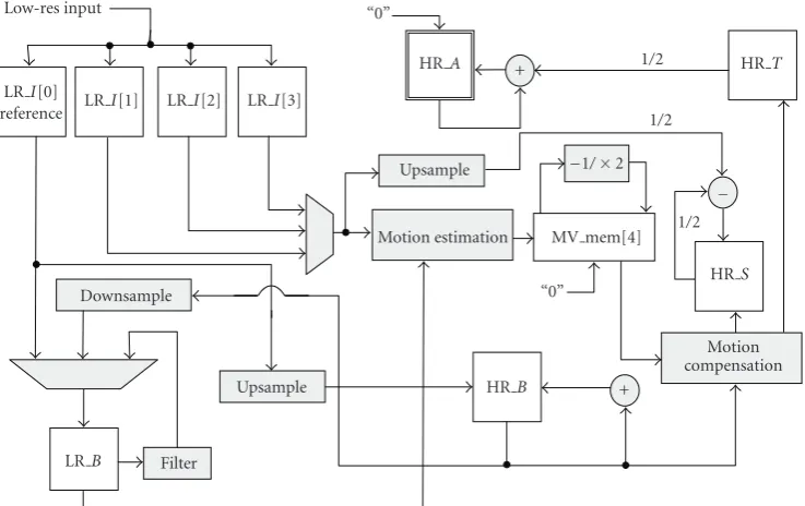
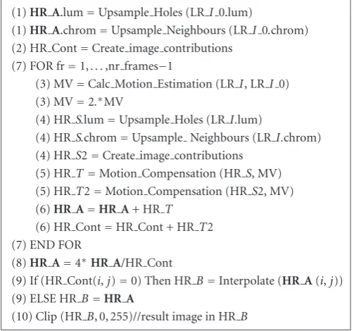
(12) Anyhow, the iterative process will stop when the maximum number of preestablished iterations is reached. Figure 5shows the ISR algorithm data flow, using the mem-ories and the resources available in the hybrid video encoder platform. The previous step numbers have been introduced between parentheses as labels at the beginning of the appro-priate lines for clearness. The memoryHRAis in boldface to remark the different bit width when compared to the other image memories.
LRB Filter
Upsample HRB +
Motion compensation Downsample
HRS “0”
1/2 MV mem[4] Motion estimation
Upsample 1/2
1/2
1/2 HRT
HRA +
“0”
LRI[0]
reference LRI[1] LRI[2] LRI[3] Low-res input
Figure5: ISR algorithm data flow.
Table1: Memory requirements of the ISR algorithm as a function of the number of the input image macroblocks.
Label ISR algorithm memory
Luminance (bits) Chrominance (bits) Total (bits)
HR A (2·MB x·2·MB y·16·16·9) (2·MB x·2·MB y·8·8·2·9) 13, 824·MB x·MB y
HRB (2·MB x·2·MB y·16·16·8) (2·MB x·2·MB y·8·8·2·8) 12, 288·MB x·MB y
HRS (2·MB x·2·MB y·16·16·8) (2·MB x·2·MB y·8·8·2·8) 12, 288·MB x·MB y
3-stripe HR (2·3·2·MB y·16·16·8) (2·3·2·MB y·8·8·2·8) 36, 864·MB y
LRB (MB x·MB y·16·16·8) (MB x·MB y·8·8·2·8) 3, 072·MB x·MB y
LRI[0] (MB x·MB y·16·16·8) (MB x·MB y·8·8·2·8) 3, 072·MB x·MB y
LRI[1] (MB x·MB y·16·16·8) (MB x·MB y·8·8·2·8) 3, 072·MB x·MB y
LRI[2] (MB x·MB y·16·16·8) (MB x·MB y·8·8·2·8) 3, 072·MB x·MB y
LRI[3] (MB x·MB y·16·16·8) (MB x·MB y·8·8·2·8) 3, 072·MB x·MB y
MV mem[0] (MB x·MB y·8) 0 8·MB x·MB y
MV mem[1] (MB x·MB y·8) 0 8·MB x·MB y
MV mem[2] (MB x·MB y·8) 0 8·MB x·MB y
MV mem[3] (MB x·MB y·8) 0 8·MB x·MB y
Total (bits) MB y·(35, 872·MB x+ 24, 576) MB y·(17, 920·MB x+ 12288) MB y·(53, 792 MB x+ 36, 864)
is the inverse of the motion between the frame and the ref-erence, increasing in this way the real motion consistency. It is interesting to highlight that the presence of aliasing in the low-resolution input images largely decreases the accuracy of the motion vectors. Due to this reason a spatial lowpass filter of order three has been applied to the input images prior to performing the motion estimation.
3.2. Implementation issues
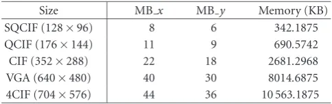
Table 1summarizes the memory requirements that the im-plementation of the ISR algorithm demands for nr frames
=4 and SF=2 as a function of the input MBs. The number
Table2: Memory requirements of the ISR algorithm for different sizes of the input image.
Size MBx MB y Memory (KB)
SQCIF (128×96) 8 6 342.1875
QCIF (176×144) 11 9 690.5742
CIF (352×288) 22 18 2681.2968
VGA (640×480) 40 30 8014.6875
4CIF (704×576) 44 36 10 563.1875
the total number of bits. The remaining memories will be multiplied by 8- bit per pixel. These requirements include four input memories as the number of frames to be com-bined has been settled upon as four. Also, a buffer containing three rows of macroblocks for reading the input images, as part of the encoder memory requirements, has been included [64]. These memory requirements also take into account the chrominance and the additional bit of HR A. The total mem-ory requirements, as a function of the number of MBs, is MB y·(6724·MB x+ 4608), expressed in bytes. Table 2 summarizes the memory requirements for the ISR algorithm with the most common input sizes. It must be mentioned that the size of the output images will be doubled in every di-rection, thus having a super-resolved image four times larger. To perform the upsample and downsample operations, it is necessary to include upsampling and downsampling blocks in hardware, being in charge of performing these op-erations on an MB basis. A hardware implementation is de-sirable as the upsample/downsample processes are very in-tensive computational tasks in the sense that they are per-formed on the entire image MBs. A software implementa-tion of these blocks could compromise the real-time per-formance, and for this reason these two tasks have been in-cluded in the texture processor. Upsampling is performed by nearest-neighbor replication from an (8×8)-pixel block to a (16×16)-pixel MB. Downsampling is achieved by picking one pixel from every set of four neighbor pixels, obtaining an 8×8 block from a 16×16 MB.
The motion estimation and motion compensation tasks are performed using the motion estimator and the motion compensator coprocessors. These coprocessors have been modified to work in quarter-pixel precision because, as it was previously established, the accuracy of the computed displacements is a critical aspect in the ISR algorithm. The arithmetic operations such as additions, subtractions, and arithmetic shifts are implemented on the texture processor. Finally, the overall control of the ISR algorithm is performed by the ARM processor which was shown inFigure 2.
4. EXPERIMENTAL SETUP
A large set of synthetic sequences have been generated with the objective of assessing the algorithm itself, independently of the image characteristics, and to enable the measurement of reliable metrics. These sequences share the following char-acteristics. Firstly, in order to isolate the metrics from the im-age peculiarities, the same frame has been replicated all over the sequence. Thus, any change in the quality will only be due
to the algorithm processing and not to the image entropy. Secondly, the displacements have been randomly generated, except for the first image of the low-resolution input set, used as the reference for the motion computation, where a null displacement is considered. This frame is used as the refer-ence in the peak signal-to-noise ratio (PSNR) computation. Finally, in order to avoid the border effects when shifting the frame, large image formats together with a later removal of the borders have been used in order to compute reliable qual-ity metrics.Figure 6depicts the experimental setup to gener-ate the test sequences [65].
The displacements introduced in the VGA images in pixel units are reflected in the low-resolution input pictures di-vided by four, that is, in quarter-pixel units. As this is the precision of the motion estimator, the real (artificially intro-duced) displacements and the ones delivered by the motion estimator are compared, in order to assess the goodness of the motion estimator used to compute the shifts among im-ages. Several sets of 40 input frames from 40 random mo-tion vectors have been generated. These synthetic sequences are used as the input for the SR process. The ISR algorithm initially performs 80 iterations over every four-input-frame set. The result is a ten-frame sequence, where each SR output frame is obtained as the combination of four low-resolution input frames.
Figure 7(a)shows the reference picture Kantoor together with the subsampled sequences that constitute the input low-resolution sequence (b), and the nearest-neighbor (c) and bilinear interpolation images (d) obtained from the first low-resolution frame (frame with zero motion vec-tor).Figure 8(a)shows the reference picture Krant together with the subsampled sequences that constitute the input low-resolution sequence (b) and the nearest-neighbor (c) and bilinear interpolations (d) obtained from the first low-resolution frame (frame with zero motion vector).
The pictures obtained with the SR algorithms are always compared to the ones obtained with the bilinear and nearest-neighbor replication interpolations in terms of PSNR. In this work, the quality of the SR algorithms are compared with the bilinear and nearest-neighbor interpolation algorithms as they suppose an alternative way to increase the image res-olution without the complexity that SR implies. The main difference between interpolation and SR is that the later adds new information from other images while the former only uses information from the same picture. The PSNR obtained with interpolation methods represents a lower bound in the sense that a PSNR above the interpolation level implies SR improvements.
Space domain PSNR Peak signal-to-noise ratio
1/2 pixel
.hvga HVGA 320240
Result
SRA tmn
2 Reference
.hvga HVGA 320240
1/2 pixel
Decimate
1/2
1/4 pixel 1/4
.qvga QVGA 160120 Subsample .vga
VGA 640480
Move
History.log Pixel shifts
.vga
VGAshift
640480
Figure6: Experimental setup for the test sequence generation.
(a) (b) (c) (d)
Figure7: (a) Reference Kantoor picture, (b) the low-resolution input sequence derived from it, (c) the nearest-neighbor, and (d) bilinear
interpolations.
(a) (b) (c) (d)
Figure8: (a) Reference Krant picture, (b) the low-resolution input sequence derived from it, (c) the nearest-neighbor, and (d) bilinear
10 9 8 7 6 5 4 3 2 1 0
Input low-resolution
Output high-resolution
8
Input low-resolution
11 10 9 8 7 6 5 4 3 2 1 0
Output high-resolution
9
2 1 0
Input low-resolution Output high-resolution
0 3
2 1 0
Input low-resolution Output high-resolution
1
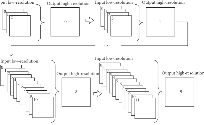
Figure9: Incremental test for assessing the SR algorithms.
1 61 121 181 241 301 361 421 481 541 601 661 721 781 Iterations
19 21 23 25 27 29 31 33 35
PSNR
(dB)
7 9
0 1 c.6 8 c.5
c.2 c.2 a a a a a c.1
2 3 4 5 6
PSNR luminance using SR
PSNR luminance using nearest-neighbor interpolation PSNR luminance using bilinear interpolation
Figure10: Luminance PSNR for 80 iterations of the Kantoor
se-quence combining 4 input frames. The output sese-quence has 10 frames.
the first frame of the Krant sequence in order to generate the low-resolution input image set, from which the super-resolved image zero is obtained. After that, a new vector is added to the previous set and these four vectors are applied again to the frame 0 of Krant to generate the super-resolved image one, based on four input low-resolution images. This process is repeated until a super-resolved image based on 12 low-resolution input frames is generated. In total, a number of 3 + 4 + 5 +· · ·+ 12=75 low-resolution frames have been used as inputs to the SR algorithms in order to generate 10 output frames.
5. ISR ALGORITHM RESULTS
In this section the test procedures exposed in the previous section have been applied to the ISR algorithm. Figure 10
shows the luminance PSNR evolution of each frame for the Kantoor sequence during the iterative process. From this chart, it is noticeable that for certain frames (frames 2 to 6) the quality rises up to a maximum value as the number of iterations increases, while for the other frames, the quality starts to rise and after a few iterations it drastically drops. The reason for this unexpected result is that the displacements were randomly generated and so, the samples presented in each frame are randomly distributed. If the samples contain all the original information (fragmented over the four input frames) then the SR process will be able to properly recon-struct the image. If some data is missing in the sampling task, then the SR process will try to adapt the SR image to the available input set, including the missing data that has been set to zero values. Higher or lower PSNR values will be obtained depending on the missing data, decreasing be-low the interpolation level (frames 7 and 9) when the avail-able data is clearly insufficient. In such cases, the ISR algo-rithm tries to match the available information to the miss-ing information within the SR frame, producmiss-ing undesirable artefacts when there is a lack of information. These artefacts cause the motion-vector field between the low-resolution version of the SR image and the low-resolution inputs to get worse with the number of iterations due to the error feed-back.
d: d.1: d.2: d.3: d.4:
c: c.1: c.2: c.3:
c.4: c.5: c.6:
b: b.1: b.2: b.3: b.4:
a:
Figure11: SR frame classification depending on the available
sam-ples.
1 61 121 181 241 301 361 421 481 541 601 661 721 781 Iterations
19 21 23 25 27 29 31 33 35
PSNR
(dB)
ISR PSNR luminance using nearest-neighbor interpolation PSNR luminance using bilinear interpolation
PSNR luminance using nearest-neighbor interpolation ISR PSNR luminance using bilinear interpolation
Figure12: Luminance PSNR for 80 iterations of the Kantoor
se-quence using nearest-neighbor and bilinear interpolations for the upsampling process.
As discussed inSection 2,Figure 12shows the PSNR of the Kantoor sequence luminance when the upsampling has been implemented using a nearest-neighbor interpolator or a bilinear interpolator. In the second case, the quality of the se-quence is lower due to the aliasing removal of the bilinear in-terpolator. Therefore, for this application a nearest-neighbor interpolator that keeps substantial amounts of aliasing across the SR process is required.
InFigure 13can be seen the average error of the motion-vector field, computed as the absolute difference between the
1 55 109 163 217 271 325 379 433 487 541 595 649 703 757 Iterations
0 2 4 6 8 10 12
Av
er
ag
e
er
ro
r
a a a a a
c.2 c.2
0 1 2 3 4 5 6 7 8 9
c.6 c.1 c.5
Figure13: Average error of the motion-vector field for 80 iterations
of the Kantoor sequence.
real motion vectors and the motion-vectors obtained by the motion estimator. The error is averaged between the hori-zontal and vertical coordinates and among all the frames. Equations (14) summarize the motion-vector error as it has been computed in this paper, where “p” is the num-ber of frames to be combined; “MB x” and “MB y” are the number of MBs in the horizontal and vertical direc-tions, respectively, and depend on the size of MB upon which the motion estimator is based; “mv·x(l)[mv x, mv y]” is the motion vector computed for the MB located at (mb x,mb y) of frame “l” in the horizontal coordinate and “mv·y(l)[mv x, mv y]” is the counterpart in the vertical coordinate. After the errors in the horizontal (error x) and vertical (error y) directions have been computed, they are averaged in a single number (error). It is clear how the er-ror decreases with the iterations for images of type “a.” For the “c.2” and “c.1” image types, the motion error drops in the beginning but it rises after a few iterations. For “c.6” and “c.5” image types, the motion error increases from the first iteration:
errorx= 1p·
p−1
l=0
1 MB x·MB y
·
MBy−1
mb y
MBx−1
mbx=0
mv·x(l)[mb x, mb y]
−mv real·x(l)[mb x, mb y] ,
error y= 1p·
p−1
l=0
1 MB x·MB y
·
MBy−1
mb y MBx−1
mbx=0
mv·y(l)[mb x, mb y]
−mv real·y(l)[mb x, mb y] , error=errorx+ error y
2 .
(14)
(a1) (b1) (a2) (b2)
Figure14: Kantoor frame number 4 of “a-type” in (a1) the spatial domain and in (b1) the frequency domain in magnitude, with their
associated errors ((a2) and (b2), resp.).
(a1) (b1) (a2) (b2)
Figure15: Krant frame number 4 of “a-type” in (a1) the spatial domain and in (b1) the frequency domain in magnitude, with their
associated errors ((a2) and (b2), resp.).
a reasonable tradeoffbetween quality and computation effort for the average cases.
If all input data are available, a maximum PSNR of 34.56 dB for frame number 4 (“a-type”) is reached for the Kantoor sequence and 37.59 dB for the Krant sequence. Figure 14shows the spatial- and frequency-domain images for Kantoor frame number 4 after 80 iterations together with the associated errors with respect to the reference, and Figure 15shows the same for frame 4 of the Krant sequence. It is clearly appreciated that the low frequencies, located in the central part of image, exhibit lower errors than the high frequencies. The reconstruction process tries to recover as much high-resolution frequencies as possible, but the low-frequency information is easier to recover, mainly be-cause almost all of such information is present prior to the SR reconstruction process.
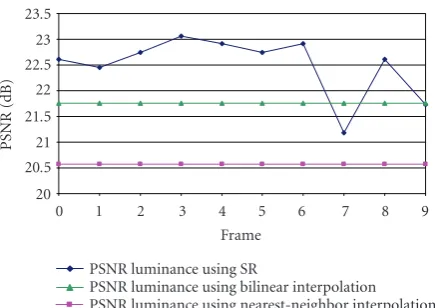
Figure 16shows the PSNR for the Kantoor sequence but by limiting the number of iterations to eight. It is easy to see that finally all the frames but one exhibit PSNR above the in-terpolation levels. Only frame 7 of type “c.6” is below such levels, whereas frame 9 of type “c.5” is just at the interpola-tion level.
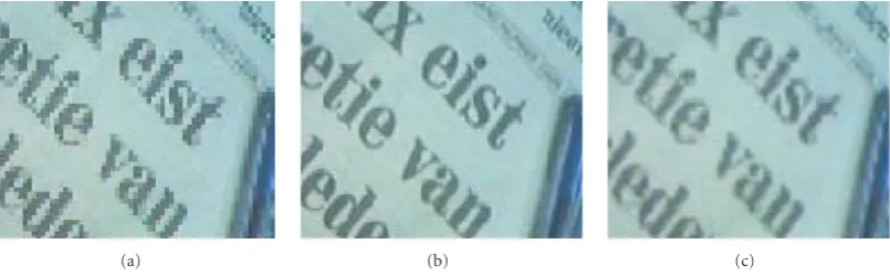
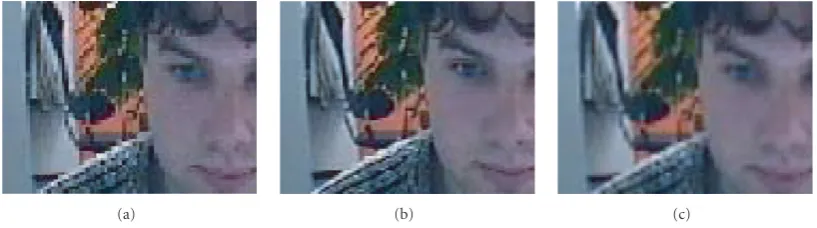
Figures17and18show some enlarged details of the Kan-toor and Krant sequences, respectively, after 80 iterations combining 4 low-resolution frames per SR output frame. In both cases, (a) is the nearest-neighbor interpolation, (b) is the SR image, and (c) is the bilinear interpolation, and also in both cases an important recovery of the high-frequency details is noticeable, as the edge recovery reveals.
Finally, the incremental test described inFigure 9was ap-plied to the ISR algorithm using the Krant sequence. Initially,
0 1 2 3 4 5 6 7 8 9
Frame 20
20.5 21 21.5 22 22.5 23 23.5
PSNR
(dB)
PSNR luminance using SR
PSNR luminance using bilinear interpolation PSNR luminance using nearest-neighbor interpolation
Figure16: PSNR of the luminance for frame 4 of the Kantoor
se-quence after 8 iterations.
(a) (b) (c)
Figure17: Enlarged details of the Kantoor sequence for frame number 4 after 80 iterations, combining 4 low-resolution frames per SR
frame. Image (a) is the nearest-neighbor interpolation, image (b) is the SR image combining 4 low-resolution input frames, and image (c) is the bilinear interpolation of the input image.
(a) (b) (c)
Figure18: Enlarged details of the Krant sequence for frame number 4 after 80 iterations, combining 4 low-resolution frames per SR frame.
Image (a) is the nearest-neighbor interpolation, image (b) is the SR image combining 4 low-resolution input frames, and image (c) is the bilinear interpolation of the input image.
represented inFigure 20is obtained. In the two cases (8 and 80 iterations), both the final and the maximum PSNR values are shown.
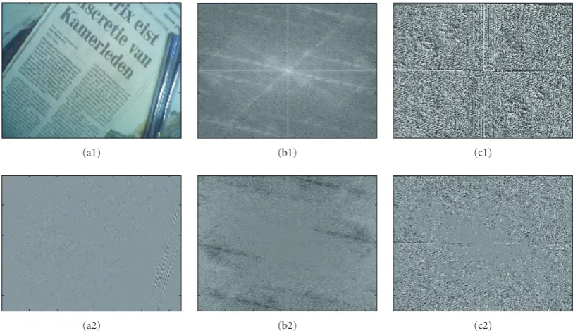
InFigure 21the SR frame number 9 is shown, as a result of the combination of 12 low-resolution frames. Image (a1) is the SR frame in the spatial domain, and (a2) is the error image when compared with the original one. Major errors are located in the edge zones, that is, in the high frequencies. The bidimensional Fourier transform in magnitude is shown in (b1) and the error image is in (b2). As expected, the cen-tral zone of the magnitude, corresponding to the lower spa-tial frequencies, exhibits the lower errors. The phase of the image is shown in (c1) together with the associated error in the frequency domain (c2). Once again, the error is mini-mal in the lower-frequency zones. Three enlarged details of the pencils of the Krant frame are shown inFigure 22: (a) the nearest-neighbor interpolation, (b) the SR image, and (c) the bilinear interpolation of the input low-resolution sequence.
6. NONITERATIVE SUPER-RESOLUTION
Although the iterative version previously described offers very good image quality when mapped onto a hybrid video encoder, the challenge is to create a new type of algorithm
that, using the same resources, could operate in a single step, that is, a noniterative algorithm suitable for real-time appli-cations. The underlying idea is based on the following con-siderations:
(i) every new image adds fresh information that must be combined into a new high-resolution grid;
(ii) it is impossible to know “a priori” (for the SR algo-rithm scope) the position of the new data and whether or not they contribute with new information.
Based on these considerations, a novel noniterative super-resolution (NISR) algorithm has been developed. This algorithm performs its operations by considering the follow-ing steps.
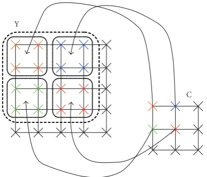
(1) Initially, the first low-resolution image is translated into a high-resolution grid, leaving the unmatched pixels to a zero value. This process will be named as “upsample holes.” As the size increases by a factor of two, both in the hori-zontal and vertical directions, the location and relationship among the pixels of high and low resolution are as shown in Figure 23.
1 39 77 115 153 191 229 267 305 343 381 419 457 495 533 571 609 647 685 723 761 799 Iterations
Combined frames
3 4 5 6 7 8 9 10 11 12
24 25 26 27 28 29 30 31 32 33 34
PSNR
(dB)
PSNR luminance using ISR
PSNR luminance using nearest-neighbor interpolation PSNR luminance using bilinear interpolation
24.48 25.18
29.54 28.68
29.84 29.11
30.45 29.77
31.24 30.34
31.46 30.76
31.88 31.07
32.54 32.51
32.78 32.72
32.81 32.71
32.90 32.78
Figure19: PSNR of the Krant sequence with 10 incremental output frames using the ISR algorithm with 80 iterations.
1 5 9 13 17 21 25 29 33 37 41 45 49 53 57 61 65 69 73 77 81 85 89 Iterations
Combined frames
3 4 5 6 7 8 9 10 11 12
25 26 27 28 29 30 31 32 33 34
PSNR
(dB)
PSNR luminance using SR
PSNR luminance using nearest-neighbor interpolation PSNR luminance using bilinear interpolation
26.53 25.88 29.54
28.68 29.84
29.06 30.45
29.73 31.24
30.34 31.46
30.81 31.88
31.21 32.57
32.80 32.83 32.90
Figure20: PSNR of the Krant sequence with 10 incremental output frames using the ISR algorithm and 8 iterations.
neighbours in the high-resolution grid. As several low-resolution images are initially combined in a grid 2-by-2 times bigger, an initial contribution of 4, for (1/2)-pixel pre-cision in low resolution, will be enough in order to keep contributions as integer values. If the resolution of the mo-tion estimator is increased or the momo-tion estimamo-tion is per-formed in high resolution, higher values will be necessary. These contributions are expressed over the high-resolution grid. The contributions of the image inFigure 23are shown in the left part ofFigure 24(b), pointing out that the original pixels have maximum contribution (four) while the rest have zero value.
(3) The relative displacements between the next input image and the first image, considered as the reference one, are estimated. These displacements are stored in a memory, as they will be used later on.
(4) Steps (1) and (2) are applied to the new input im-age, that is, it is adapted to the high-resolution grid, leaving
the missing pixels to zero and generating the initial contribu-tions.
(5) In this step, both the new image over the high-resolution grid and its associated contributions are motion compensated towards the reference image. The real contribu-tions of the new pixels to the high-resolution reference image will be reflected in the compensated contributions.
(6) The arithmetical addition between the initial image and the compensated images is performed. The same process is completed with initial and compensated contributions. This summation assures further noise reduction in the re-sulting image.
(7) Steps (3) to (6) are applied to the next incoming im-ages.
(a1) (b1) (c1)
(a2) (b2) (c2)
Figure21: Super-resolved image after combining 12 low-resolution frames in (a1) the spatial domain, in (b1) the magnitude frequency
domain, and in (c1) the phase frequency domain, together with their associated errors ((a2), (b2), and (c2)) for the Krant sequence.
(a) (b) (c)
Figure22: Enlarged details of the nearest-neighbor interpolation of (a) the input image, (b) the SR image after combining 12 low-resolution
input frames, and (c) the bilinear interpolation of the input image for the Krant sequence.
high-resolution image is adjusted depending on the contri-butions, as it is indicated in (15), whereNis the number of frames to be combined, SR(i,j) is the SR image, LR Iis the low-resolution input image and contributions represents the contributions memory.
SR(i,j)=N
·
N
fr=1Motion Compensate
Upsample HolesLR I[fr] N
fr=1Motion Compensate
contributions[fr] . (15)
Assigning to the accumulative memory HR A a length of 12 bits, 16 frames can be safely stored in it. In the worst case, an accumulation of a value of 255 will be performed, which multiplied by 16 gives 4080, fitting in 12 bits.
(9) After the adjustment, it is possible that some pixel po-sitions remain empty, because certain popo-sitions from the
in-put image set did not add new information. This case will be denoted by a zero, both in the high-resolution image position and in the contributions. The only solution to this problem is to interpolate the zeroes with the surrounding informa-tion. However, the presence of a zero in the image does not necessarily implies that such value must be interpolated, be-cause zero is a possible and valid value in an image. Due to this reason, a pixel will be interpolated only if its final contri-bution is zero.
Table3: Memory requirements of the NISR as a function of the number of the input image macro-blocks.
Label NISR algorithm memory
Luminance (bits) Chrominance (bits) Total (bits)
HR A (2·MB x·2·MB y·16·16·12) (2·MB x·2·MB y·8·8·2·12) 18, 432·MB x·MB y
HRB (2·MB x·2·MB y·16·16·8) (2·MB x·2·MB y·8·8·2·8) 12, 288·MB x·MB y
HRS (2·MB x·2·MB y·16·16·8) (2·MB x·2·MB y·8·8·2·8) 12, 288·MB x·MB y
HRS2 (2·MB x·2·MB y·16·16·8) (2·MB x·2·MB y·8·8·2·8) 12, 288·MB x·MB y
HR Cont (2·MB x·2·MB y·16·16·8) (2·MB x·2·MB y·8·8·2·8) 12, 288·MB x·MB y
3-stripe HR (2·3·2·MB y·16·16·8) (2·3·2·MB y·8·8·2·8) 36, 864·MB y
LRI[0] (MB x·MB y·16·16·8) (MB x·MB y·8·8·2·8) 3, 072·MB x·MB y
LRI[1] (MB x·MB y·16·16·8) (MB x·MB y·8·8·2·8) 3, 072·MB x·MB y
MV mem[0] (MB x·MB y·8) 0 8·MB x·MB y
Total (bits) MB y·(49, 160·MB x+ 24, 576) MB y·(24, 576·MB x+ 12288) MB y·(73, 736 MB x+ 36, 864)
Lowresolution Highresolution
Figure 23: Mapping of the low-resolution pixels in the
high-resolution grid, leaving holes for the missing pixels.
Table4: Memory requirements of the NISR algorithm for different
sizes of the input image.
Size MBx MB y Memory (KB)
SQCIF (128×96) 8 6 459.0468
QCIF (176×144) 11 9 931.5966
CIF (352×288) 22 18 3645.3867
VGA (640×480) 40 30 10 936.1718
4CIF (704×576) 44 36 14 419.5468
video encoder. MemoryHRAis in boldface to remark the different bit width when compared to the other memories. The block-diagram has been divided into two different parts: on the left side is the zone dedicated to the image processing, which makes use of memories HR A, HRT, HRS, LRI 0, and LRI, besides storing the motion vectors in MV ref2fr. On the right side is the zone dedicated to the contributions processing, which makes use of memories HRS2, HRT2, and HR Cont. In order to clarify the relationships among them, the image data flow has been drawn in solid lines, the
Y
C
(a)
Luminance contributions:
4 0
0 0
Chrominance contributions:
4 4
4 4 (b)
Figure 24: (a) Mapping of the chrominance C to the
high-resolution grid by means of replicating the pixels and its relation-ship with the luminance Y. (b) Initial contributions of the lumi-nance and chromilumi-nance images.
contribution data flow in dotted lines, and the motion-vector flow in dashed lines. Moreover, the functions “upsample” and “motion compensation” have been superscripted with an asterisk to point out their different behaviors when they are executing in the SR mode.
6.1. Implementation issues
(1)HR A.lum=Upsample Holes (LRI 0.lum)
(1)HR A.chrom=Upsample Neighbours (LRI 0.chrom)
(2) HR Cont=Create image contributions
(7) FOR fr=1,. . .,nr frames−1
(3) MV=Calc Motion Estimation (LRI, LRI 0) (3) MV=2.∗MV
(4) HRS.lum=Upsample Holes (LRI.lum)
(4) HRS.chrom=Upsample Neighbours (LRI.chrom)
(4) HRS2=Create image contributions
(5) HRT=Motion Compensation (HRS, MV)
(5) HRT2=Motion Compensation (HRS2, MV)
(6)HR A=HR A+ HRT
(6) HR Cont=HR Cont + HRT2
(7) END FOR
(8)HR A=4∗HR A/HR Cont
(9) If (HR Cont(i,j)=0) Then HRB=Interpolate (HR A(i,j))
(9) ELSE HRB=HR A
(10) Clip (HRB, 0, 255)//result image in HRB
Algorithm2: Pseudocode of the NISR algorithm implemented on the video encoder.
Motion
estimation 2 MV ref2fr mv
Motion compensation
HRT2 LRI Upsample HRS
Motion compensation
Create contributions
HRT HRS2
Images +
HR Cont +
LRI 0
reference Upsample
HR A 4
Contributions HRB Interpolate
Figure25: NISR algorithm data flow.
Table 3summarizes the memory requirements that the NISR algorithm requests. Compared with the ISR it can be appreciated that now there are five high-resolution memo-ries instead of three, although the low-resolution and motion estimation memories have been reduced from four to two and from four to one, respectively.Table 4 summarizes the memory requirements of the NISR algorithm for the most common input sizes.
6.1.1. Adjustments in the motion compensator
Y
C
Figure26: Relationship between the chrominance and the
lumi-nance for sampling format YCbCr 4 : 2 : 0.
and due to the lower attention of the human eye to the bor-ders when compared with the centre of the images, this effect is negligible. However, to obtain SR improvements the artifi-cial introduction of nonexisting data results in quality degra-dation in the borders. The solution is to modify the motion compensator to fill the empty values with zeroes, so that the NISR algorithm has an opportunity to fill the holes with valid values coming from other images.
6.1.2. Adjustments in the chrominances
Due to the different sampling schemes used for the lumi-nance and the chromilumi-nance components, it is necessary to perform some modifications on the proposed NISR algo-rithm to obtain SR improvements also in the chrominance images.
First of all, for the chrominance pixels, the way to per-form the upsampling process cannot be the same as the one used with the luminance. This fact is reflected inFigure 26, where it can be seen how each chrominance pixel affects four luminance pixels. Therefore, when the chrominance high-resolution grid is generated, every pixel must be replicated four times in order to keep the chromatic coherence as shown inFigure 24(a).
For the same reason, the initial chrominance contribu-tions cannot be the same as the luminance ones. As there is no zero-padding, all the chrominance pixels must ini-tially have the same contribution weights, as is shown in Figure 24(b) where the initial contributions for the lumi-nance and the chromilumi-nances are presented.
7. NONITERATIVE RESULTS
In order to enable a suitable comparison between the ISR and the NISR algorithms, firstly the results of combining four low-resolution frames per output SR frame will be shown for both sequences. InFigure 27the PSNR resulting from apply-ing the NISR algorithm to the Kantoor sequence is shown
0 1 2 3 4 5 6 7 8 9
Frame 18
23 28 33 38 43 48 53
PSNR
(dB)
PSNR luminance using NISR
PSNR luminance using bilinear interpolation PSNR luminance using nearest-neighbor interpolation
Figure27: PSNR of the NISR when combining four low-resolution
images per frame for the Kantoor sequence.
0 1 2 3 4 5 6 7 8 9
Frame 20
25 30 35 40 45 50 55
PSNR
(dB)
PSNR luminance using NISR
PSNR luminance using bilinear interpolation PSNR luminance using nearest-neighbor interpolation
Figure28: PSNR of the NISR when combining four low-resolution
images per frame for the Krant sequence.
andFigure 28shows the SR results for the Krant sequence. As far as the introduced shifts have been the same for both sequences, they exhibit a very similar behavior. The first one has an average PSNR of 36.07 dB, while the second one has an average PSNR of 38.47 dB. The quality differences are due to the inherent nature of these two images: in the same con-ditions, a lower entropy image will always have higher PSNR. InFigure 29is shown the resulting frame number 4 in the case of the Kantoor sequence, as it exhibits the higher quality of the ten-frame sequence. As it was commented inSection 5, the error is again lower in the low-frequency region. Com-pared with the ISR algorithm, the error image for the NISR algorithm is more uniform both in the spatial and in the fre-quency domain for the same number of combined frames. A detailed observation of the same frame for the Krant se-quence offers the same results, as it can be seen inFigure 30. At the same time, some details of these last images contain-ing edges are shown both for Kantoor and Krant sequences in Figures31and32, respectively, increasing in both cases the perceptual quality.
(a1) (b1) (c1)
(a2) (b2) (c2)
Figure29: PSNR of the NISR when combining four low-resolution frames for the Kantoor sequence.
(a1) (b1) (c1)
(a2) (b2) (c2)
Figure30: PSNR of the NISR when combining four low-resolution frames for the Krant sequence.
The perceptual quality exhibits few variations after combin-ing 6 input frames, that is, when 34.57 dB is reached. In ad-dition, it can be seen that the largest increment in the quality (the greatest PSNR slope) takes place in the first four output frames. All the established facts lead to the conclusion that a NISR system can be limited to combine 5 or 6 input frames, depending on the available resources and the desired output quality.
(a) (b) (c)
Figure31: Enlarged detail of the Kantoor sequence with 10 output frames when four low-resolution frames are combined.
(a) (b) (c)
Figure32: Enlarged detail of the Krant sequence with 10 output frames when four low-resolution frames are combined.
3 4 5 6 7 8 9 10 11 12
Combined frames 24
26 28 30 32 34 36 38
PSNR
(dB)
PSNR luminance using SR
PSNR luminance using bilinear interpolation PSNR luminance using nearest-neighbor interpolation 27.69
29.21 32.56
34.57 35.82
35.79 36.56
37.62 38.08 38.45
24.48 25.18
Figure33: Incremental test of the Krant sequence with 10 output
frames.
phase spectral error (c2) follows the same trend. When com-paring these results with the ones shown inFigure 35(which have been obtained combining only 3 low-resolution frames) higher amounts of aliasing and consequently, higher error with respect with the original image, are perceived.
InFigure 36 an enlarged detail of the frame shown in Figure 34is shown, obtained as the gathering of 12 frames by the NISR algorithm. In (a) the nearest-neighbor interpo-lation is shown, in (b) the SR image and in (c) the bilinear in-terpolation. The quality improvement of the image, is clearly manifested, especially for those letters on the top right side of the super-resolved image.
8. ALGORITHMS COMPARISON
The two developed SR algorithms have been compared through three main features: the simulation time (measured in milliseconds), the obtained quality (measured in PSNR dB), and the memory requirements (measured in MB).
(a1) (b1) (c1)
(a2) (b2) (c2)
Figure34: Super-resolved frame after combining 12 low-resolution frames in (a1) the spatial domain, in (b1) the frequency domain in
magnitude, and in (c1) phase, together with their associated errors((a2), (b2), and (c2)).
(a1) (b1) (c1)
(a2) (b2) (c2)
Figure35: Super-resolved frame after combining 3 low-resolution frames in (a1) the spatial domain, in (b1) the frequency domain in
magnitude, and in (c1) phase, together with their associated errors ((a2), (b2), and (c2)).
With respect to the quality exhibited by each SR algo-rithm, it is interesting to remark that it is important to con-sider not only the absolute value of the PSNR achieved by the algorithm but also the quality increase with respect to the interpolation levels, as it represents the SR gain with re-spect to a cheaper and faster method to increase the image size. InFigure 38a comparison between the quality obtained