A Probabilistic Model for Learning Multi-Prototype Word Embeddings
Fei Tian†, Hanjun Dai∗, Jiang Bian‡, Bin Gao‡,Rui Zhang?, Enhong Chen†, Tie-Yan Liu‡
†University of Science and Technology of China, Hefei, P.R.China ∗Fudan University, Shanghai, P.R.China
‡Microsoft Research, Building 2, No. 5 Danling Street, Beijing, P.R.China
?Sun Yat-Sen University, Guangzhou, P.R.China
†[email protected],†[email protected],∗[email protected], ‡{jibian, bingao, tyliu}@microsoft.com,?[email protected]
Abstract
Distributed word representations have been widely used and proven to be useful in quite a few natural language processing and text mining tasks. Most of existing word embedding models aim at generating only one embedding vector for each individual word, which, however, limits their effectiveness because huge amounts of words are polysemous (such asbankandstar). To address this problem, it is necessary to build multi embedding vectors to represent different meanings of a word respectively. Some recent studies attempted to train multi-prototype word embeddings through clustering context window features of the word. However, due to a large number of parameters to train, these methods yield limited scalability and are inefficient to be trained with big data. In this paper, we introduce a much more efficient method for learning multi embedding vectors for polysemous words. In particular, we first propose to model word polysemy from a probabilistic perspective and integrate it with the highly efficient continuous Skip-Gram model. Under this framework, we design an Expectation-Maximization algorithm to learn the word’s multi embedding vectors. With much less parameters to train, our model can achieve comparable or even better results on word-similarity tasks compared with conventional methods.
1 Introduction
Distributed word representations usually refer to low dimensional and dense real value vectors (a.k.a. word embeddings) to represent words, which are assumed to convey semantic information contained in words. With the exploding text data on the Web and fast development of deep neural network technolo-gies, distributed word embeddings have been effectively trained and widely used in a lot of text mining tasks (Bengio et al., 2003) (Morin and Bengio, 2005) (Mnih and Hinton, 2007) (Collobert et al., 2011) (Mikolov et al., 2010) (Mikolov et al., 2013b).
While word embedding plays an increasingly important role in many tasks, most of word embedding models, which assume one embedding vector for each individual word, suffer from a critical limitation for modeling tremendous polysemous words (e.g. bank,left,doctor). Using the same embedding vec-tor to represent the different meanings (we will call prototypeof a word in the rest of the paper) of a polysemous word is somehow unreasonable and sometimes it even hurts the model’s expression ability.
To address this problem, some recent efforts, such as (Reisinger and Mooney, 2010) (Huang et al., 2012), have investigated how to obtain multi embedding vectors for the respective different prototypes of a polysemous word. Specifically, these works usually take a two-step approach: they first train single prototype word representations through a multi-layer neural network with the assumption that one word only yields single word embedding; then, they identify multi word embeddings for each polysemous word by clustering all its context window features, which are usually computed as the average of single prototype embeddings of its neighboring words in the context window.
Compared with traditional single prototype model, these models have demonstrated significant im-provements in many semantic natural language processing (NLP) tasks. However, they suffer from a This work is licenced under a Creative Commons Attribution 4.0 International License. Page numbers and proceedings footer are added by the organizers. License details:http://creativecommons.org/licenses/by/4.0/
crucial restriction in terms of scalability when facing exploding training text corpus, mainly due to the deep layers and huge amounts of parameters in the neural networks in these models. Moreover, the performance of these multi-prototype models is quite sensitive to the clustering algorithm and requires much effort in clustering implementation and parameter tuning. The lack of probabilistic explanation also refrains clustering based methods from being applied to many text mining tasks, such as language modeling.
To address these challenges, in this work, we propose a new probabilistic multi-prototype model and integrate it into a highly efficient continuous Skip-Gram model, which was recently introduced in the well-known Word2Vec toolkit (Mikolov et al., 2013b). Compared with conventional neural network language models which usually set up a multi-layer neural network, Word2Vec merely leverages a three-layer neural network to learn word embeddings, resulting in greatly decreased number of parameters and largely increased scalability. However, similar to most of existing word embedding models, Word2Vec also assumesone embedding for one word. We break this limitation by introducing a new probabilistic framework which employs hidden variables to indicate which prototype each word belongs to in the con-text. In this framework, the conditional probability of observing wordwOconditioned on the presence
of neighboring wordwI (i.e. P(wO|wI)) can be formulated as a mixture model, wheremixtures
corre-sponds towI’s differentprototypes. This is a more natural way to defineP(wO|wI), since it has taken the
polysemy of wordwI into consideration. After defining the model, we design an efficient
Expectation-Maximization (EM) algorithm to learn various word embedding vectors corresponding to each ofwI’s
prototypes. Evaluations on widely used word similarity tasks demonstrate that our algorithm produces comparable or even better word embeddings compared with either clustering-based multi-prototype mod-els or the original Skip-Gram model. Furthermore, as a unified way to obtain multi word embeddings, our proposed method can effectively avoid the sensitivity to the clustering algorithm applied by previous multi-prototype word embedding approach.
The following of the paper is organized as follows: we introduce related work in Section 2. Then, Section 3 describes our new model and algorithm in details and conducts a comparison in terms of complexity between our algorithm and the previous method. We present our experimental results in Section 4. The paper is concluded in Section 5.
2 Related Work
Since the initial work (Bengio et al., 2003), there have been quite a lot of neural network based models to obtain distributed word representations (Morin and Bengio, 2005) (Mnih and Hinton, 2007) (Mikolov et al., 2010) (Collobert et al., 2011) (Mikolov et al., 2013b). Most of these models assume that one word has only one embedding, except the work of Eric Huang (Huang et al., 2012), in which the authors propose to leverage global context information and multi-prototype embeddings to achieve performance gains in word similarity task. To obtain multi-prototype word embeddings, this work conducts clustering on a word’s all context words’ features in the corpus. The features are the embedding vectors trained previously via a three-layer neural network. Each cluster’s centroid is regarded as the embedding vector for each prototype. Their reported experimental results verify the importance of considering multi-prototype models.
Note that (Reisinger and Mooney, 2010) also proposes to deal with the word polysemy problem by assigning to each prototype a real value vector. However their embedding vectors are obtained through a tf-idf counting model, which is usually called as distributional representations (Turian et al., 2010), rather than through a neural network. Therefore, we do not regard their paper as very related to our work. The similar statement holds for other works on vector model for word meaning in context such as (Erk and Pad´o, 2008) (Thater et al., 2011) (Reddy et al., 2011) (Van de Cruys et al., 2011).
Our model is mainly based on the recent proposed Word2Vec model, more concretely, the continuous Skip-Gram model (Mikolov et al., 2013a) (Mikolov et al., 2013b). The continuous Skip-Gram model specifies the probability of observing the context words conditioned on the central wordwI in the
3 Model Description
In this section, we introduce our algorithm for learning multi-prototype embeddings in details. In partic-ular, since our new model is based on the continuous Skip-Gram model, we first make a brief introduction to the Skip-Gram model. Then, we present our new multi-prototype algorithm and how we integrate it into the Skip-Gram model. After that, we propose an EM algorithm to conduct the training process. We also conduct a comparison on the number of parameters between the new EM algorithm and the state-of-the-art multi-prototype model proposed in (Huang et al., 2012), which can illustrate the efficiency superior of our algorithm.
3.1 Multi-Prototype Skip-Gram Model
In contrast to the conventional ways of using context words to predict the next word or the central word, the Skip-Gram model (Mikolov et al., 2013b) aims to leverage the central word to predict its context words. Specifically, assuming that the central word iswI and one of its neighboring word iswO,
P(wO|wI)is modeled in the following way:
P(wO|wI) = exp(V T wIUwO)
∑w∈Wexp(VwTIUw)
, (1)
whereWdenotes the dictionary consisting of all words,Uw∈RdandVw∈Rdrepresent thed-dimensional
‘output’ and ‘input’ embedding vectors of wordw, respectively. Note that all the parameters to be learned are the input and output embedding vectors of all words, i.e. U={Uw|w∈W}andV ={Vw|w∈W}.
This corresponds to a three-layer neural network, in whichUandVdenote the two parameter matrices of the neural network. Compared with the conventional neural networks employed in the literature which yield at least four layers (including the look-up table layer), the Skip-Gram model greatly reduces the number of parameters and thus gives rise to a significant improvement in terms of training efficiency.
Our proposed Multi-Prototype Skip-Gram model is similar to the original Skip-Gram model in that it also aims to modelP(wO|wI)and uses two matrices (the input and output embedding matrices) as the
parameters. The difference lies in that given wordwI, the occurrence of wordwOis described as a finite
mixture model, in which each mixture corresponds to a prototype of wordwI. To be specific, suppose
that wordwhasNwprototypes and it appears in itshw-th prototype, i.e.,hw∈ {1,···,Nw}is the index of
w’s prototype. ThenP(wO|wI)is expanded as:
p(wO|wI) = NwI
∑
i=1P(wO|hwI=i,wI)P(hwI=i|wI) (2)
=
NwI
∑
i=1exp(UT wOVwI,i)
∑w∈Wexp(UwTVwI,i)
P(hwI =i|wI), (3)
whereVwI,i∈Rdrefers to the embedding vector ofwI’si-th prototype. This equation states thatP(wO|wI)
is a weighted average of the probabilities of observingwOconditioned on the appearance ofwI’s every
prototype. The probability P(wO|hwI =i,wI) takes the similar softmax form to equation (1) and the
weight is specified as a prior probability of wordwIfalls in its every prototype.
The general idea behind the Multi-Prototype Skip-Gram model is very intuitive: the surrounding words under different prototypes of the same word are usually different. For example, when the word bank refers to the side of a river, it is very possible to observe the corresponding context words such as river, water, and slope; however, when bank falls into the meaning of the financial organization, the surrounding word set is likely to be comprised of quite different words, such as money, account, and investment.
The probability formulation in (3) brings much computation cost because of the linear dependency of
|W|in the denominator∑w∈Wexp(UwTVwI,i). To address this issue, several efficient methods have been
Softmax Tree as an example, through a binary tree in which every word is a leaf node, word wO is
vector associated with thet-th node in the path from the root to the leaf nodewO. Substituting (4) into
(2) to replace the large softmax operator in (3) leads to a much more efficient probability form.
3.2 EM Algorithm
In this section, we describe the EM algorithm adopted to train the Multi-Prototype Skip-Gram model. Without loss of generality, we will focus on obtaining multi embeddings for a specified word w∈W with Nw prototypes. Wordw’s embedding vectors are denoted as Vw∈Rd×Nw. Suppose there are M
word pairs for training:{(w1,w),(w2,w),···,(wM,w)}, where all the inputs words (i.e., wordw) are the
same, and the set of output words to be predicted are denoted asX={w1,w2,···,wM}. That is,XareM
surrounding words ofwin the training corpus.
For ease of reference and without loss of generality, we make some changes to the notations in Section 3.1. We will use hm as the index of w’s prototype in the pair (wm,w), m∈ {1,2,···,M}. Besides,
is the t-th bit of the binary coding vector of word walong its corresponding path on the Hierarchical Softmax Tree.
With equation (5), the E-Step and M-Step are:
E-Step:
TheQfunction w.r.t. the parameters at thei-th iterationθ(i)is written as:
πk=∑ M m=1γˆm,k
M , k=1,2···,Nw. (8) We leave the detailed derivations for equation (6), (7), and (8) to the appendix of the paper. Then we discuss how we obtain the update of the embedding parametersUwm,tandVw,k. Note that the optimization
problem is non-convex, and it is hard to compute the exact solution of∂U∂wm,tQ =0 and∂∂VQw,k =0. Therefore, we use gradient ascent to optimize in the M-step. The gradients ofQfunction w.r.t. embedding vectors are given by:
∂Q
∂Uwm,t
=
∑
Nwk=1
ˆ
γm,kb(twm) 1−ς(bt(wm)UwTm,tVw,k)
Vw,k, (9)
∂Q
∂Vw,k = M
∑
m=1γˆm,kLwm
∑
t=1b(wm)
t 1−ς(bt(wm)UwTm,tVw,k)
Uwm,t. (10)
Iterating betweenE-StepandM-Steptill the convergence of the value of functionQmakes the EM algorithm complete.
In order to enhance the scalability of our approach, we propose a fast computing method to boost the implementation of the EM algorithm. Note that the most expensive computing operations in both the E-Step and M-Step are the inner product of the input and output embedding vectors, as well as the sigmoid function. However, if we take the Hierarchical Softmax Tree form as shown in Equation (4) to modelP(wm|hm=i,w), and perform only one step gradient ascent in M-Step, the aforementioned two
expensive operations in M-Step will be avoided by leveraging the pre-computed results in the E-Step. Specifically, since the gradient of the function f(x) =logς(x)is given by f0(x) =1−ς(x), the sigmoid
values computed in the E-Step to obtainP(wm|hm=i,w)(i.e. the termς(bt(wm)UwTm,tVw,k)in equation (5),
(9), and (10)) can be re-used to derive the gradients in the M-Step.
However, such enhanced computation method cannot benefit the second order optimization methods in the M-Step such as L-BFGS and Conjugate Gradient, since they usually rely on multiple iterations to converge. In fact, we tried these two optimization methods in our experiments but they have brought no improvement compared with simple one-step gradient ascent method.
3.3 Model Comparison
To show that our model is more scalable than the former multi-prototype model in (Huang et al., 2012) (We denote it as EHModel in the rest of the paper), we conduct a comparison on the number of parameters with respect to each of these two models in this subsection.
We usenembeddingandnwindowto denote the numbers of all word embedding vectors and context
win-dow words, respectively. It is clear thatnembeddings=∑w∈WNw. EHModel aims to compute two scores,
i.e., the local score and the global score, both with hidden layer node activations. We denote the hidden layer node number ashlandhgfor these two scores. The parameter numbers are listed in Table 1.
Model EHModel Our Model
#parameters dnwords+dnembeddings+ (dnwindow+1)hl+ (2d+1)hg dnwords+dnembeddings
Table 1: Comparison of parameter numbers of two models
Note that d in Table 1 denotes the embedding vector size. It can be observed that EHModel has (dnwindow+1)hl+ (2d+1)hgmore parameters than our model, which is mainly because EHModel has
one more layer in the neural network and it considers global context. In previous study (Huang et al., 2012),d,nwindow,hl, andhgare set to be 50, 10, 100, 100, respectively, which greatly increases the gap
4 Experiments
In this section, we will present our experimental settings and results. Particularly, we first describe the data collection and the training configuration we used in the experiments; then, we conduct a qualitative case study followed by quantitative evaluation results on a public word similarity task to demonstrate the performance of our proposed model.
4.1 Experimental Setup
Dataset: To make a fair comparison with the state-of-the-art methods, we employ a publicly available dataset, which is used in (Huang et al., 2012), to train word embeddings in our experiments. Particularly, this training corpus is a snapshot of Wikipedia at April, 2010 (Shaoul, 2010), which contains about 990 million tokens. We removed the infrequent words from this corpus and kept a dictionary of about 1 million most frequent words. Similar to Word2Vec, we removed pure digit words such as2014as well as about 100 stop words likehow,for, andwe.
Training Configuration: In order to boost the training speed, we take advantage of the Hierarchical Softmax Tree structure. More concretely, we use the Huffman tree structure, as introduced in Word2Vec, to further increase the training speed. All the embedding size, including both word embedding vectors and the Huffman tree node embedding vectors, are set to be 50, which is the same as the size used in (Huang et al., 2012). To train word embedding, we set the context window size as 10, i.e., for a wordw, 10 of the closest neighboring words toware regarded asws contexts. For the numbers of word prototypes, i.e.,Nwintroduced in Section 3.2, we set the top 7 thousand frequent words as multi-prototype words by
experience, with all of them having 10 prototypes (i.e.Nw=10).
During the training process, we used the same strategy to set the learning rate as what Word2Vec did. Specifically, we set the initial learning rate to 0.025 and diminished the value linearly along with the increasing number of training words. Our experimental results illustrate that this learning rate strategy can lead to the best results for our algorithm.
For the hyper parameters of the EM algorithm, we set the batch size to 1, i.e. M=1 in Section 3.2, since our experimental results reveal that smaller batch size can result in better experimental results. The reason is explained as the following. Our optimization problem is highly non-convex. Smaller batch size yields more frequent updates of parameters, and thus avoids trapping in local optima, while larger batch size, associated with more infrequent parameter updating, may cause higher probability to encounter local optima. In our experiments, we observe that only one iteration of E-Step and M-Step can reach the embedding vectors with good enough performance on the word similarity task, whereas increasing the iteration number just leads to slight performance improvement with much longer training time. Under the above configuration, our model runs about three times faster than EHModel.
4.2 Case Study
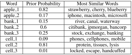
This section gives some qualitative evaluations of our model by demonstrating how our model can ef-fectively identify multi-prototype word embeddings on some specific cases. In Table 2, we list several polysemous words. For each word, we pick some of their prototypes learned by our model, including the prototype prior probability (i.e. πi introduced in Section 3.2) and three of the most similar words
with each prototype, respectively. The similarity is calculated by the cosine similarity score between the embedding vectors.
From the table we can observe some interesting results of the multi-prototype embedding vectors produced by our model:
• For a polysemous word, its different embedding vectors represent its different semantic meanings. For example, the first embedding vector of the wordapplecorresponds to its sense as a kind of fruit, whereas the second one represents its meaning as an IT company.
Word Prior Probability Most Similar Words apple 1 0.82 strawberry, cherry, blueberry apple 2 0.17 iphone, macintosh, microsoft bank 1 0.15 river, canal, waterway bank 2 0.6 citibank, jpmorgan, bancorp bank 3 0.25 stock, exchange, banking
cell 1 0.09 phones, cellphones, mobile cell 2 0.81 protein, tissues, lysis cell 3 0.01 locked, escape, handcuffed
Table 2: Most similar words with different prototypes of the same word
0.09) orprisoned(with probability 0.01). Note that the three prior probability scores ofcelldo not sum to 1. The reason is that there are some other embeddings not presented in the table which are found to have high similarities with the three embeddings. We do not present them due to the space limitation.
• By setting the prototype number to a fairly large value (e.g. Nw=10), the model tends to learn
more fine-grained separations of the word’s different meanings. For example, we can observe from Table 2 that the second and the third prototypes of the wordbankseem similar to each other as both of them denote a financial concept. However, there are subtle differences between them: the second prototype represents concrete banks, such as citibank and jpmorgan, whereas the third one denotes what is done in the banks, since it is most similar to the wordsstock,exchange, andbanking. We believe that such a fine-grained separation will bring more expressiveness to the multi-prototype word embeddings learned by our model.
4.3 Results on Word Similarity in Context Dataset
In this subsection, we give quantitative comparison of our method with conventional word embedding models, including Word2Vec and EHModel (Huang et al., 2012).
The task we perform is the word similarity evaluation introduced in (Huang et al., 2012). Word simi-larity tasks evaluate a model’s performance by calculating the Spearman’s rank correlation between the ranking of ground truth similarity scores (given by human labeling) and the ranking based on the simi-larity scores produced by the model. Traditional word simisimi-larity tasks such as WordSim353 (Finkelstein et al., 2001) and RG (Rubenstein and Goodenough, 1965) are not suitable for evaluating multi-prototype models since there is neither enough number of polysemous words in these datasets nor context infor-mation to infer the prototype index. To address this issue, a new word similarity benchmark dataset including context information was released in (Huang et al., 2012). Following (Luong et al., 2013), we use SCWS to denote this dataset. Similar to WordSim353, SCWS contains some word pairs (concretely, 2003 pairs), together with human labeled similarity scores for these word pairs. What makes SCWS different from WS353 is that the words in SCWS are contained in sentences, i.e., there are 2003 pairs of sentences containing these words, while words in WS353 are not associated with sentences. Therefore, the human labeled scores are based on the meanings of the words in the context. Given the presence of the context, the word similarity scores, especially those scores depending on polysemous words, are much more convincing for evaluating different models’ performance in our experiments.
Then, we propose a method to compute the similarity score for a pair of words{w1,w2}in the context
based on our model. Suppose that the context of a wordwis defined as all its neighboring words in a T+1 sized window, wherewis the central word in the window. We useContext1={c11,c12,···,c1T}and
Context2={c21,c22,···,c2T} to separately denote the context ofw1 andw2, where ct1andc2t are thet-th
context word ofw1andw2, respectively. According to Bayesian rule, we have that fori∈ {1,2,···,Nw1}:
P(hw1 =i|Context1,w1)∝P(Context1|hw1 =i,w1)P(hw1 =i|w1)
=
∏
Tt=1P(c 1
where P(c1
t|hw1 =i,w1) can be calculated by equation (4) and P(hw1 =i|w1) is the prior probability
we learned in the EM algorithm (equation (8)). The similar equation holds for wordw2 as well. Here
we make an assumption that the context words are independent with each other given the central word. Furthermore, suppose that the most likely prototype index for w1 givenContext1 is ˆhw1, i.e., we
de-note ˆhw1 =argmaxi∈{1,2,···,Nw1}P(hw1 =i|Context1,w1). Similarly, ˆhw2 is denoted as the corresponding
meaning forw2.
We calculate two similarity scores base on equation (11), i.e., MaxSim Score and WeightedSim Score: MaxSim(w1,w2) =Cosine(Vw1,hˆw1,Vw2,hˆw2), (12)
WeightedSim(w1,w2) =
Nw1
∑
i=1Nw2
∑
j=1P(hw1=i|Context1,w1)P(hw2 =j|Context2,w2)Cosine(Vw1,i,Vw2,j).
(13) In the above similarity scores,Cosine(x,y) denotes the cosine similarity score of vectorxandy, and Vw,i∈Rdis the embedding vector for the wordw’si-th prototype.
The detailed experimental results are listed in Table 3, where ρ refers to the Spearman’s rank cor-relation. The higher value ofρ indicates the better performance. The performance score of EHModel is borrowed from its original paper (Huang et al., 2012). For Word2Vec model, we use Hierarchical Huffman Tree rather than Negative Sampling to do the acceleration. OurModel Muses the MaxSim score in testing and ourModel Wuses the WeightedSim score. All of these models are run on the same aforementioned Wikipedia corpus, with the dimension of the embedding space to be 50.
From the table, we can observe that ourModel W(65.4%) outperforms the original Word2Vec model (61.7%), and achieves almost the same performance with the state-of-the-art EHModel (65.7%). Among the two similarity measures used in testing, the WeightedSim score performs better (65.4%) than the MaxSim score (63.6%), indicating that the overall consideration of all prototype probabilities are more effective.
Model ρ×100 Word2Vec 61.7
EHModel 65.7 Model M 63.6 Model W 65.4
Table 3: Spearman’s rank correlations on SCWS dataset.
5 Conclusion
In this paper, we introduce a fast and probabilistic method to generate multiple embedding vectors for polysemous words, based on the continuous Skip-Gram model. On one hand, our method addresses the drawbacks of the original Word2Vec model by leveraging multi-prototype word embeddings; on the other hand, our model yields much less complexity without performance loss compared with the former clustering based multi-prototype algorithms. In addition, the probabilistic framework of our method avoids the extra efforts to perform clustering besides training word embeddings.
For the future work, we plan to apply the proposed probabilistic framework to other neural network language models. Moreover, we would like to apply the multi-prototype embeddings to more real world text mining tasks, such as information retrieval and knowledge mining, with the expectation that the multi-prototype embeddings produced by our model will benefit these tasks.
References
Yoshua Bengio, R´ejean Ducharme, Pascal Vincent, and Christian Janvin. 2003. A neural probabilistic language model. InJournal of Machine Learning Research, pages 1137–1155.
Katrin Erk and Sebastian Pad´o. 2008. A structured vector space model for word meaning in context. In Proceed-ings of the Conference on Empirical Methods in Natural Language Processing, EMNLP ’08, pages 897–906, Stroudsburg, PA, USA. Association for Computational Linguistics.
Lev Finkelstein, Evgeniy Gabrilovich, Yossi Matias, Ehud Rivlin, Zach Solan, Gadi Wolfman, and Eytan Ruppin. 2001. Placing search in context: The concept revisited. InProceedings of the 10th international conference on World Wide Web, pages 406–414. ACM.
Eric H Huang, Richard Socher, Christopher D Manning, and Andrew Y Ng. 2012. Improving word representations via global context and multiple word prototypes. In Proceedings of the 50th Annual Meeting of the Associa-tion for ComputaAssocia-tional Linguistics: Long Papers-Volume 1, pages 873–882. Association for Computational Linguistics.
Minh-Thang Luong, Richard Socher, and Christopher D Manning. 2013. Better word representations with recur-sive neural networks for morphology.CoNLL-2013, 104.
Tomas Mikolov, Martin Karafi´at, Lukas Burget, Jan Cernock`y, and Sanjeev Khudanpur. 2010. Recurrent neural network based language model. InINTERSPEECH, pages 1045–1048.
Tomas Mikolov, Kai Chen, Greg Corrado, and Jeffrey Dean. 2013a. Efficient estimation of word representations in vector space. arXiv preprint arXiv:1301.3781.
Tomas Mikolov, Ilya Sutskever, Kai Chen, Greg S. Corrado, and Jeff Dean. 2013b. Distributed representations of words and phrases and their compositionality. In C.J.C. Burges, L. Bottou, M. Welling, Z. Ghahramani, and K.Q. Weinberger, editors,Advances in Neural Information Processing Systems 26, pages 3111–3119.
Andriy Mnih and Geoffrey Hinton. 2007. Three new graphical models for statistical language modelling. In
Proceedings of the 24th international conference on Machine learning, pages 641–648. ACM.
Andriy Mnih and Koray Kavukcuoglu. 2013. Learning word embeddings efficiently with noise-contrastive esti-mation. In C.J.C. Burges, L. Bottou, M. Welling, Z. Ghahramani, and K.Q. Weinberger, editors,Advances in Neural Information Processing Systems 26, pages 2265–2273.
Frederic Morin and Yoshua Bengio. 2005. Hierarchical probabilistic neural network language model. In Proceed-ings of the international workshop on artificial intelligence and statistics, pages 246–252.
Siva Reddy, Ioannis P Klapaftis, Diana McCarthy, and Suresh Manandhar. 2011. Dynamic and static prototype vectors for semantic composition. InIJCNLP, pages 705–713.
Joseph Reisinger and Raymond J Mooney. 2010. Multi-prototype vector-space models of word meaning. In
Human Language Technologies: The 2010 Annual Conference of the North American Chapter of the Association for Computational Linguistics, pages 109–117. Association for Computational Linguistics.
Herbert Rubenstein and John B Goodenough. 1965. Contextual correlates of synonymy. Communications of the ACM, 8(10):627–633.
Westbury C Shaoul, C. 2010. The westbury lab wikipedia corpus.
Stefan Thater, Hagen F¨urstenau, and Manfred Pinkal. 2011. Word meaning in context: A simple and effective vector model. InIJCNLP, pages 1134–1143.
Joseph Turian, Lev Ratinov, and Yoshua Bengio. 2010. Word representations: a simple and general method for semi-supervised learning. In Proceedings of the 48th Annual Meeting of the Association for Computational Linguistics, pages 384–394. Association for Computational Linguistics.
Tim Van de Cruys, Thierry Poibeau, and Anna Korhonen. 2011. Latent vector weighting for word meaning in context. InProceedings of the Conference on Empirical Methods in Natural Language Processing, EMNLP ’11, pages 1012–1022, Stroudsburg, PA, USA. Association for Computational Linguistics.
6 Appendix
6.1 Derivations for the EM Algorithm
According to the properties of conditional probability, we have
From equation (7), theQfunction is calculated as: Q(θ,θ(i)) =E[logP(X,Γ|Θ)|Θ(i)]
Then we give the derivations for π’s updating rule, i.e., equation (8). Note that for parametersπk,
k={1,2,···,Nw}, they need to satisfy the condition that∑Nk=w1πk=1. From equation (7) (or equivalently
equation (15)), the loss with regard toπis:
L[π]=
∑
Mwhereλ is the Language multiplier. Letting ∂L[π]
∂π =0, we obtain:
πk∝ M
∑
m=1γˆm,k. (17)
Further considering the fact that∑Nw
k=1∑Mm=1γˆm,k=M, we haveπk=∑ M m=1γˆm,k