A Beam-Search Decoder for Disfluency Detection
Xuancong Wang1,3 Hwee Tou Ng1,2Khe Chai Sim2 1NUS Graduate School for Integrative Sciences and Engineering 2Department of Computer Science, National University of Singapore 3Human Language Technology, Institute for Infocomm Research, Singapore [email protected], {nght, simkc}@comp.nus.edu.sg
Abstract
In this paper1, we present a novel beam-search decoder for disfluency detection. We first
pro-pose node-weighted max-margin Markov networks (M3N) to boost the performance on words belonging to specific part-of-speech (POS) classes. Next, we show the importance of measur-ing the quality of cleaned-up sentences and performmeasur-ing multiple passes of disfluency detection. Finally, we propose using the beam-search decoder to combine multiple discriminative models such as M3N and multiple generative models such as language models (LM) and perform multi-ple passes of disfluency detection. The decoder iteratively generates new hypotheses from current hypotheses by making incremental corrections to the current sentence based on certain patterns as well as information provided by existing models. It then rescores each hypothesis based on features of lexical correctness and fluency. Our decoder achieves an edit-word F1 score higher than all previous published scores on the same data set, both with and without using external sources of information.
1 Introduction
Disfluency detection is a useful and important task in Natural Language Processing (NLP) because spon-taneous speech contains a significant proportion of disfluency. The disfluencies in speech introduce noise in downstream tasks like machine translation and information extraction. Thus, the task of disfluency detection not only can help improve the readability of automatically transcribed speech, but also the performance of downstream NLP tasks.
There are mainly two types of disfluencies: filler words and edit words. Filler words include filled pauses (e.g., ‘uh’, ‘um’) and discourse markers (e.g., “I mean”, “you know”). They are insertions in spontaneous speech that indicate pauses or mark boundaries in discourse. Thus, they do not convey useful content information. Edit words are words that are spoken wrongly and then corrected by the speaker. For example, consider the utterance:
I want a flight
Edit z }| {
to Boston
Filler z }| {
uh I mean
Repair z }| {
to Denver
The phrase “to Boston” forms the edit region to be replaced by “to Denver”. The words “uh I mean” are filler words that serve to cue the listener about the error and subsequent correction. So, the cleaned-up sentence would be “I want a flight to Denver”, which is what the speaker originally intended to say. In general, edit words are more difficult to detect than filler words, and so edit word prediction accuracy is much lower. Thus, in this work, we mainly focus on edit word detection.
In Section 2, we briefly introduce previous work. In Section 3, we describe our improved baseline system that will be integrated into our beam-search decoder. Section 4 presents our beam-search decoder in detail. In Section 5, we describe our experiments and results. Section 6 gives the conclusion.
1The research reported in this paper was carried out as part of the PhD thesis research of Xuancong Wang at the NUS Graduate School for Integrated Sciences and Engineering.
This work is licensed under a Creative Commons Attribution 4.0 International Licence. Page numbers and proceedings footer are added by the organisers. Licence details:http://creativecommons.org/licenses/by/4.0/
2 Previous Work
Researchers have tried many models for disfluency detection. Johnson and Charniak (2004) proposed a TAG-based (Tree-Adjoining Grammar) noisy channel model, which showed great improvement over a boosting-based classifier (Charniak and Johnson, 2001). Maskey et al. (2006) proposed a phrase-level machine translation approach for this task. Liu et al. (2006) used conditional random fields (CRFs) (Laf-ferty et al., 2001) for sentence boundary and edit word detection. They showed that CRFs significantly outperformed maximum entropy models and hidden Markov models (HMM). Zwarts and Johnson (2011) extended this model using minimal expected F-loss oriented n-best reranking. Georgila (2009) presented a post-processing method during testing based on integer linear programming (ILP) to incorporate local and global constraints. In addition to textual information, prosodic features extracted from speech have been incorporated to detect edit words in some previous work (Kahn et al., 2005; Liu et al., 2006; Zhang et al., 2006). Zwarts and Johnson (2011) also trained extra language models on additional corpora, and compared the effects of adding scores from different language models as features during reranking. They reported that the language models gained approximately 3% in F1-score for edit word detection on the Switchboard development dataset. Qian and Liu (2013) proposed multi-step disfluency detection using weighted max-margin Markov networks (M3N) and achieved the highest F-score of 84.1% without using any external source of information. In this paper, we incorporate the M3N model into our beam-search decoder framework with some additional features to further improve the result.
3 The Improved Baseline System
Weighted max-margin Markov networks (M3N) (Taskar et al., 2003) have been shown to outperform CRF in (Qian and Liu, 2013), since it can balance precision and recall easily by assigning different loss penalty to different label misclassification pairs. In this work, we made use of M3N in expanding the search space and rescoring the hypotheses. To facilitate the integration of the M3N system into our decoder framework, we made several modifications that slightly improve the M3N baseline system. Our improved baseline system has two stages: the first stage is filler word prediction using M3N to detect words which can potentially be fillers, and the second stage is joint edit and filler word prediction using M3N. The output of the first stage is passed as features into the second stage. Both stages perform filler word prediction, since we found that joint edit and filler word detection performs better than edit word detection alone as edit words tend to co-occur with filler words, and the first-stage output can be fed into the second stage to extract additional features. We also augmented the M3N toolkit to support additional feature functions, allow weighting of individual nodes, and control the total number of model parameters.2
3.1 Node-Weighted and Label-Weighted Max-Margin Markov Networks (M3N)
A max-margin Markov network (M3N) (Taskar et al., 2003) is a sequence labeling model. It has the same structure as conditional random fields (CRF) (Lafferty et al., 2001) but with a different objective function. A CRF is trained to maximize the conditional probability of the true label sequence given the observed input sequence, while an M3N is trained to maximize the difference between the conditional probability of the true label sequence and the incorrectly predicted label sequence (i.e., maximizing the margin). Thus, we can regard M3N as a support vector machine (SVM) analogue of CRF (Suykens and Vandewalle, 1999).
The dual form of the training objective function of M3N is formulated as follows:
min α
1 2Ck
X
x,y
αx,y∆f(x,y)k22+
X
x,y
αx,yL(x,y)
s.t. X
y
αx,y= 1,∀x and αx,y≥0,∀x,y
(1)
wherexis the observed input sequence,y∈ Yis the output label sequence,αx,y are the dual variables
to be optimized, andC ≥ 0is the regularization parameter to be tuned. ∆f(x,y) =f(x,ye)−f(x,y¯) is the residual feature vector, whereeyis the true label sequence,y¯ is the predicted label sequence given the model, andf(x,y)is the feature vector. It is implemented as a sum over all nodes:
f(x,y) =X t
f(x,y, t) (2)
where tis the position index of the node in the sequence. Each component of f(x,y, t) is a feature function,f(x,y, t). For example,f(w0=‘so’, y0=‘F’, y−1=‘O’, t)has a value of 1 only when the word at nodetis ‘so’, the label at nodetis ‘F’ (filler word), and the label at node(t−1)is ‘O’ (outside edit/filler region, i.e., fluent). The maximum length of theyhistory (for this feature function, it is 2 since onlyy0 andy−1 are covered) is called theclique orderof the feature. L(x,y)is the loss function. A standard M3N uses an unweighted hamming loss, which is the number of incorrect nodes:
L(x,y) =X t
δ(yet,y¯t) whereδ(a, b) =
(
1, ifa=b
0, otherwise (3)
Qian and Liu (2013) proposed using label-weighted M3N to balance precision and recall by adjusting the penalty on false positives and false negatives, i.e.,v(yet,y¯t)in Eqn. 4. In this work, we further extend this technique to individual nodes to train expert models, each specialized in a specific part-of-speech (POS) class. Our loss function is:
L(x,y) =X t
uc(t)v(eyt,y¯t)δ(yet,y¯t) whereuc(t) =
(
Bc, if POS(t)∈Sc
1, otherwise (4)
whereBcis a factor which controls the extent to which the model is biased to minimize errors on specific nodes, POS(t)is the POS tag of the word at nodet, andScis the set of POS tags corresponding to that expert classc. We show that by integrating these expert models into our decoder framework, we can achieve further improvement.
3.2 Features
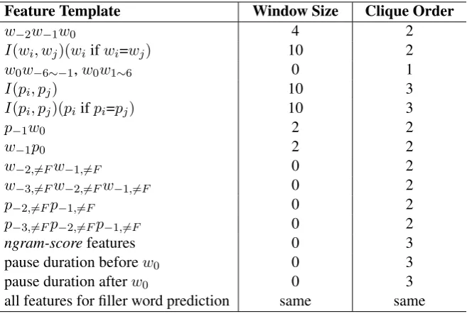
The feature templates for filler word and edit word prediction are listed in Table 1 and Table 2 re-spectively. wi refers to the word at the ith position relative to the current node; window size is the maximum number of words before and after the current word that the template covers, e.g., w−1w0 with a window size of 4 meansw−4w−3, w−3w−2, ..., w3w4; pi refers to the POS tag at the ith po-sition relative to the current node; wi∼j refers to any word from the ith position to the jth position relative to the current node; wi,6=F refers to the ith word (w.r.t. the current node) not being a filler word; the multi-pair comparison function I(a, b, c, ...) indicates whether each pair (a andb, b andc, and so on) are identical, for example, ifa = b 6= c = d, it will output “101” (‘1’ for being equal, ‘0’ for being unequal); and ngram-scorefeatures are the natural logarithm of the following probabilities:
P(w−3, w−2, w−1, w0),P(w0|w−3, w−2, w−1),P(w−3, w−2, w−1),P(h/si|w−3, w−2, w−1),P(w−3),
P(w−2),P(w−1),P(w0)(“h/si” denotes sentence-end). We use language models (LM) in two ways: individual n-gram scores as M3N features, and an overall sentence-level score for rescoring in our beam-search decoder. Our experiments show that this way of using LM gives the best performance.
Feature Template Window Size Clique Order
w0 4 1
w−1w0 4 2
I(wi, wj) 10 2
I(wi, wj, wi+1, wj+1) 10 2
p0 4 1
p−1p0 4 2
p−2p−1p0 4 2
I(pi, pj) 10 2
I(pi, pj, pi+1, pj+1) 10 2
[image:4.595.156.441.61.215.2]transitions 0 3
Table 1: Feature templates for filler word prediction
Feature Template Window Size Clique Order
w−2w−1w0 4 2
I(wi, wj)(wiifwi=wj) 10 2
w0w−6∼−1,w0w1∼6 0 1
I(pi, pj) 10 3
I(pi, pj)(piifpi=pj) 10 3
p−1w0 2 2
w−1p0 2 2
w−2,6=Fw−1,6=F 0 2
w−3,6=Fw−2,6=Fw−1,6=F 0 2
p−2,6=Fp−1,6=F 0 2
p−3,6=Fp−2,6=Fp−1,6=F 0 2
ngram-scorefeatures 0 3
pause duration beforew0 0 3
pause duration afterw0 0 3
all features for filler word prediction same same Table 2: Feature templates for edit word prediction
4 The Beam-Search Decoder Framework
4.1 Motivation
[image:4.595.136.465.246.467.2]disfluency detection to overcome these limitations.
POS Freq. (%) Edit F1 (%) PRP 25.5 92.33
DT 14.2 88.95
IN 10.4 84.45
VBP 8.3 86.88
RB 7.1 81.78
CC 4.6 86.76
BES 4.2 93.37
NN 3.4 52.30
VBD 3.1 86.51
VB 2.1 70.42
VBZ 1.9 79.70
[image:5.595.218.381.86.267.2]... ... ...
Table 3: Baseline edit F1 scores for different POS tags
4.2 General Framework
The goal of the decoder is to find the best hypothesis for a given input sentence w. A hypothesis h is a label sequence, one label for every word in the sentence. To find the best hypothesis, the decoder iteratively generates new hypotheses from current ones using a set ofhypothesis producersand rescores each hypothesis using a set ofhypothesis evaluators. For each hypothesis produced, the decoder cleans up the sentence by removing all the predicted filler words and edit words so that subsequent operations can act on the cleaned-up sentencew¯ if needed. Each hypothesis evaluator produces a scoref which measures the quality of the current hypothesis based on certain aspects of fluency specific to that hypoth-esis evaluator. The overall score of a hypothhypoth-esis is the weighted sum of the scores from all the hypothhypoth-esis evaluators:
score(h,w) =X i
λifi(h,w) (5)
The weights λis are tuned on the development set using minimum error rate training (MERT) (Och, 2003). The decoding algorithm is shown in Algorithm 1.
In our description, hi denotes the hypothesized label at theith position; wi denotes the word at the
ith position;|h|denotes the length of the label sequence;f
M3N(hi,w) denotes the M3N log-posterior probability of the label (at theith position of hypothesish) being the hypothesized label; fM3N(h,w)
denotes the normalized joint log probability of hypothesishgiven the M3N model (‘normalized’ means divided by the length of the label sequence);w¯ denotes the cleaned-up sentence;fLM(w¯) =fLM(h,w) denotes the language model score of the sentencew¯ (cleaned up according to hypothesish) divided by sentence length; and¯hdenotes the sub-hypothesis obtained by running M3N on the cleaned-up sentence with updated features. Note that a sub-hypothesis will have a shorter label sequence if some words are labeled as filler word or edit word in the parent hypothesis. We can obtain hfrom ¯hby inserting all predicted filler and edit words from the parent hypothesis into the sub-hypothesis so that its label sequence has the same length as the original sentence.
4.3 Hypothesis Producers
The goal of hypothesis producers is to create a search space for rescoring using various hypothesis eval-uators. Based on the information provided by the existing models and certain patterns where disfluencies may occur, we propose the following hypothesis producers for our beam-search decoder:
Algorithm 1
The beam-search decoding algorithm for a sentence. S: hypothesis stack;h: hypothesis;f: hypothe-sis evaluator score vector;Λ: hypothesis evaluator weight vector
INPUT: a sentencewwithN words
OUTPUT: a sequence ofN labels, from{E, F, O}
1: initialize hypothesish0,hi=‘O’∀i∈[1, N] 2: SA← {h0}, SB ← ∅
3: foriter= [1,maxIter]do 4: for eachhinSAdo
5: for eachproducerin hypothesisProducersdo 6: for eachh0inproducer(h)do
7: computef(h0,w)from hypothesisEvaluators
8: computescore(h0,w) =Λ>·f(h0,w)
9: SB←SB+{h0} 10: pruneSBaccording toscore 11: SA←SB, SB=∅
12: returnargmaxh{score(h,w)},h∈SA
phrases (up to 5 words) and their corresponding true labels by considering the most frequent incorrectly predicted phrases in the development set. During decoding, whenever such a phrase occurs in a sentence and its label is not the same as that in the dictionary, it is changed to that in the dictionary and a new hypothesis is produced. For example, if the phrase “you know” has occurred 1144 times and has been misclassified 31 times, out of which 9 times it should be ‘O’, then an entry “you know O||1144 31 9” will be added to the dictionary. If the original sentence contains “you know” and it is not labeled as O, a new hypothesis will be generated by labeling it as ‘O’.
Repetition: Whenever the ith word and the jth word (j > i) are the same, all words from theith position (inclusive) to thejthposition (exclusive) are labeled as edit words. For example, in “I want to be able to um I just want it more for multi-tasking”, three hypotheses are produced. The first hypothesis is produced by labeling every word in “I want to be able to um” as edit words since ‘I’ is repeated. The second hypothesis is produced by labeling every word in “want to be able to um I just” as edit words since ‘want’ is repeated. The third hypothesis is produced by labeling “to be able” as edit words since ‘to’ is repeated. The window size within which we search for repetitions is set to 12 (i.e.,j−i≤12), since the longest edit region (due to repetition) in the development set is of that size. We introduce this hypothesis producer because the baseline system tends to miss long edit regions, especially when very few words in the region are repeated. However, sometimes a speaker does change what he intends to say by aborting a sentence so that only the beginning few words are repeated, as in the above sentence.
Filler-word-marker: We trained an M3N model for filler word detection. Multiple passes of filler word detection on cleaned-up sentences can sometimes detect filler words that are missed in earlier passes. This hypothesis producer runs before every iteration starts. It performs filler word prediction and modifies the feature table by setting the filler-indicator feature to true so that subsequent operations see the updated feature. However, it does not remove filler words during the clean up process because some words are defined as both filler word and edit word simultaneously.
Edit-word-marker: We run our baseline M3N (the second stage) on the cleaned-up sentence and obtain theN-best hypotheses, i.e., the top N hypothesesh with max{fM3N(¯h,w¯)}. This producer essentially performs multiple passes of disfluency detection.
4.4 Hypothesis Evaluators
Our decoder uses the following hypothesis evaluators to select the best hypothesis:
texts (both filler words and edit words are removed). This score measures the fluency of the resulting cleaned-up sentence w.r.t. a fluent language model.
Disfluent language model score: This is the normalized language model score of the cleaned-up sen-tence, i.e., fdisfluentLM(w¯). A 4-gram language model is trained on the original training texts which contain disfluencies. This score measures the fluency of the resulting cleaned-up sentence w.r.t. a disflu-ent language model. These two LM scores provide contrastive measures because if a cleaned up sdisflu-entence still contains disfluencies, the disfluent LM will be preferred over the fluent LM.
M3N disfluent score: This is the normalized joint log probability score of the current hypothesish, i.e.,fM3N(h,w). This score measures how much the baseline M3N model favors the disfluency label assignment of the current hypothesis.
M3N fluent score: This is the normalized joint log probability score of labeling the entire cleaned-up sentence as fluent, i.e.,
fM3N(¯h=O,w¯) = |1¯h|
|¯h| X
i=1
fM3N(¯hi=‘O’,w¯) (6)
This score measures how much the baseline M3N model favors the cleaned-up sentence of the current hypothesis. It acts as a discriminative LM in measuring the fluency of the cleaned-up sentence. If the cleaned-up sentence contains disfluencies, this evaluator function will tend to give a lower score.
Expert-POS-classcdisfluent score: This is the normalized joint log probability score of the current hypothesishunder the expert M3N model for POS classcdynamically combined with the baseline M3N model, i.e.,
fc(h,w) = |h1|
|h| X
i=1
gc(hi,w), gc(hi,w) =
(
fM3N-c(hi,w)if POS(wi)∈Sc
fM3N(hi,w)if POS(wi)∈/Sc (7)
Training of the expert M3N models is described in Section 4.6. 4.5 Integrating M3N into the Decoder Framework
In most previous work such as (Liu et al., 2006) and (Qian and Liu, 2013) that performed filler and edit word detection using sequence models, the begin-inside-end-single (BIES) labeling scheme was adopted, i.e., for edit words (E), 4 labels are defined: E B (beginning of an edit region), E I (inside an edit region), E E (end of an edit region), and E S (single-word edit region). However, since our beam-search decoder needs to change the labels dynamically among filler words, edit words, and fluent words, it will be problematic if the label sequence has to conform to the BIES constraint especially when the posteriors are concerned. Thus, we use the minimal set of labels: E (Edit word), F (Filler word), O (Outside edit and filler region).
For the first-stage filler word detection, only ‘F’ and ‘O’ are used. To compensate for degradation in performance, we increase the clique order of features to 3. We found that increasing the clique order has a similar effect as using the BIES labeling scheme. For example, f(wi=‘so’, y0=‘E B’, t) means the previous word is not an edit, both the current word and the next word are edit words, i.e., the previous word, the current word, and the next word can be either O-E-E or F-E-E. So in our mini-mal labeling scheme, this feature will be decomposed intof(wi=‘so’, y−1=‘O’, y0=‘E’, y+1=‘E’, t)and
f(wi=‘so’, y−1=‘F’, y0=‘E’, y+1=‘E’, t), both having a higher clique order.
Our preliminary experiments show that by increasing the clique order of features while reducing the number of labels (keeping about the same total number of parameters), we can maintain the same per-formance. However, training takes a longer time.
4.6 POS-Class Specific Expert Models
the corresponding POS class. That is, M3N-Expert-POS-class-1 is trained to optimize performance on words belonging to POS-class-1. Nonetheless, it can still predict disfluency for words in other POS classes, except that the error rate may be higher because of the way training is biased.
Class POS tags Freq. (%) F1 range
1 RBS POS PDT NNPS HVS PRP$ BES PRP 33.5 92.3 – 100
2 MD EX CC DT VBP WP WRB 32.2 86.0 – 90.8
3 RB IN 16.7 82.8 – 83.8
4 TO VBD WDT RP JJS 5.1 80.0 – 82.1
5 VBZ VB VBN JJ 6.1 69.3 – 78.1
[image:8.595.254.345.594.650.2]6 VBG NN CD JJR UH NNS NNP XX RBR 3.2 42.1 – 64.2 Table 4: POS classes for expert M3N models and their baseline F1 scores
We split all POS tags into 6 classes, by first sorting all POS tags in descending order of their F1 scores. Next, for POS tags with higher F1 scores, we form larger classes (higher total proportion), and for POS tags with lower F1 scores, we form smaller classes. The POS classes are shown in Table 4. The algorithm dynamically selects posteriors from different M3N models, depending on the POS tag of the current word.
5 Experiments
5.1 Experimental Setup
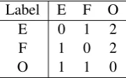
We tested all the systems on the Switchboard Treebank corpus (LDC99T42), using the same train/develop/test split as previous work (Johnson and Charniak, 2004; Qian and Liu, 2013). We removed all partial words and punctuation symbols to simulate the condition when automatic speech recognition (ASR) output is used. Our training set contains 1.3M words in 174K sentences; our development set contains 86K words in 10K sentences; and our test set contains 66K words in 8K sentences. The original system has high precision but low recall, i.e., the system tends to miss out edit words. The imbalance can be solved by setting a larger penalty for mis-labeling edits as fluent, i.e., 2 instead of 1 for the weighted hamming loss. We used the loss matrix, v(yet,y¯t), in Table 5 to balance precision and recall. We set the biasing factorBcto 2, for every classc. We also added two pause duration features (pause duration before and after the current word) from the corresponding Switchboard speech corpus (LDC97S62). We trained our acoustic model on the Fisher corpus and used it to perform forced alignment on the Switch-board corpus to obtain the word boundary time information for calculating pause durations. For the ngram-scorefeatures, we used the small 4-gram language model trained on the training set with filler words and edit words removed. All continuous features are quantized into 10 discrete bins using cumu-lative binning (Liu et al., 2006). We setmaxIterto 4 in Algorithm 1. The regularization parameterC
is set to 0.006, obtained by tuning on the development set.
Label E F O
E 0 1 2
F 1 0 2
O 1 1 0
Table 5: Weighted hamming loss,v(yet,y¯t)for M3N for both stages
5.2 Results
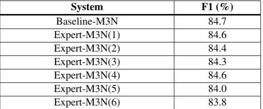
will sacrifice the overall performance on the entire data set especially on POS classes with lower baseline scores (see Table 7). But since we have several expert models, if we combine them, they can complement each other’s weakness and give an overall slightly better performance. The result also shows that the gain by training expert models decreases as the baseline performance on that POS class increases. For example, POS class 6 has the poorest baseline performance and the gain is 2.1%. This gain decreases gradually as we move up the table rows because the baseline performance gets better.
POS class Expert-M3N F1 Baseline-M3N F1
1 92.5 92.2
2 87.1 86.9
3 84.9 84.7
4 85.3 84.1
5 71.8 70.4
[image:9.595.163.437.154.254.2]6 57.3 55.2
Table 6: Edit detection F1 scores (%) of expert models on all words belonging to that POS class in the test set (expert-M3N column), and baseline model on all words belonging to that POS class in the test set (baseline-M3N column)
System F1 (%)
Baseline-M3N 84.7
Expert-M3N(1) 84.6
Expert-M3N(2) 84.4
Expert-M3N(3) 84.3
Expert-M3N(4) 84.6
Expert-M3N(5) 84.0
Expert-M3N(6) 83.8
Table 7: Degradation of the overall performance by expert models compared to the baseline model
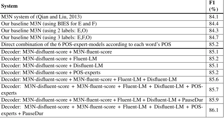
Table 8 shows the performance comparison of our baseline models and our beam-search decoder. Statistical significance tests show that our best decoder model incorporating all hypothesis evaluators gives a higher F1 score than the 3-label baseline M3N model (statistically significant atp <0.001), and the 3-label baseline M3N model gives a higher F1 score than the M3N system of (Qian and Liu, 2013) (statistically significant at p = 0.02). Our three baseline models have about the same total number of parameters (7.6M). The BIES baseline M3N system uses the same feature templates as shown in Table 2 with reduced clique order. The 2-label baseline M3N system uses the same feature templates with the same clique order. Our results also show that joint filler and edit word prediction performs 0.4% better than edit word prediction alone. Direct combination of expert models is done by first running the general model and the expert models on each sentence to obtain all the label sequences (one for each model). Then for every word in the sentence, if its POS belongs to any one of those POS classes, we choose its label from the output of the corresponding expert model; otherwise, we choose its label from the output of the baseline model.
[image:9.595.164.436.322.435.2]System F1(%)
M3N system of (Qian and Liu, 2013) 84.1
Our baseline M3N (using BIES for E and F) 84.4
Our baseline M3N (using 2 labels: E,O) 84.3
Our baseline M3N (using 3 labels: E,F,O) 84.7
Direct combination of the 6 POS-expert-models according to each word’s POS 85.2 Decoder: M3N-disfluent-score + M3N-fluent-score 85.1
Decoder: M3N-disfluent-score + Fluent-LM 85.2
Decoder: M3N-disfluent-score + Disfluent-LM 85.1 Decoder: M3N-disfluent-score + POS-experts 85.2 Decoder: M3N-disfluent-score + M3N-fluent-score + Fluent-LM + Disfluent-LM 85.6 Decoder: M3N-disfluent-score + M3N-fluent-score + Fluent-LM + Disfluent-LM +
POS-experts 85.7
Decoder: M3N-disfluent-score + M3N-fluent-score + Fluent-LM + Disfluent-LM + PauseDur 85.9 Decoder: M3N-disfluent-score + M3N-fluent-score + Fluent-LM + Disfluent-LM +
[image:10.595.76.529.64.309.2]POS-experts + PauseDur 86.1
Table 8: Performance of the beam-search decoder with different combinations of components
than our baseline M3N model (single-threaded). Overall, it took about 0.4 seconds to detect disfluencies in one sentence with our proposed beam-search decoder approach.
To the best of our knowledge, the best published F1 score on the Switchboard Treebank corpus is 84.1% (Qian and Liu, 2013) without the use of external sources of information, and 85.7% (Zwarts and Johnson, 2011) with the use of external sources of information (large language models from additional corpora were used in (Zwarts and Johnson, 2011)). Without the use of external sources of information, our decoder approach achieves an F1 score of 85.7%, significantly higher than the best published F1 score of 84.1% of (Qian and Liu, 2013). Our decoder approach also achieves an F1 score of 86.1% after adding external sources of information (pause duration features), higher than the F1 score of 85.7% of (Zwarts and Johnson, 2011).
5.3 Discussion
We have manually analyzed the improvement of our decoder over the M3N baseline. For example, consider the sentence in Table 9. Both the baseline M3N system and the first pass output of the decoder will give the cleaned-up sentence “are these do these programs ...”, which is still disfluent and has a relatively lower fluent LM score but a relatively higher disfluent LM score because of the erroneous n-gram “are these do these”. The decoder makes use of the fluent LM and disfluent LM hypothesis evaluators during the beam search and performs additional passes of cleaning and eventually gives the correct output.
Sentence Um and uh are these like uh do these programs ...
Reference F F F E E E F O O O ...
M3N baseline F F F O O F F O O O ...
Decoder F F F E E E F O O O ...
Table 9: An example showing the effect of measuring the quality of the cleaned-up sentence.
the sentence in multiple passes. Hypothesis evaluators corresponding to expert models achieve the pur-pose of combining POS class-specific expert models. All of these components extend the flexibility of the decoder framework in performing disfluency detection.
6 Conclusion
In conclusion, we have proposed a search decoder approach for disfluency detection. Our beam-search decoder performs multiple passes of disfluency detection on cleaned-up sentences. It evaluates the quality of cleaned-up sentences and use it as a feature to rescore hypotheses. It also combines multiple expert models to deal with edit words belonging to a specific POS class. In addition, we also proposed a way (using node-weighted M3N in addition to label-weighted M3N) to train expert models each focusing on minimizing errors on words belonging to a specific POS class. Our experiments show that combining the outputs of the expert models directly according to POS tags can give rise to some improvement. Combining the expert model scores with language model scores in a weighted manner using our beam-search decoder achieves further improvement. To the best of our knowledge, our decoder has achieved the best published edit-word F1 score on the Switchboard Treebank corpus, both with and without using external sources of information.
7 Acknowledgments
This research is supported by the Singapore National Research Foundation under its International Re-search Centre @ Singapore Funding Initiative and administered by the IDM Programme Office.
References
Eugene Charniak and Mark Johnson. 2001. Edit detection and parsing for transcribed speech. InProc. of NAACL.
Daniel Dahlmeier and Hwee Tou Ng. 2012. A beam-search decoder for grammatical error correction. InProc. of EMNLP-CoNLL.
Kallirroi Georgila. 2009. Using integer linear programming for detecting speech disfluencies. InProc. of NAACL.
Mark Johnson and Eugene Charniak. 2004. A TAG-based noisy channel model of speech repairs. InProc. of ACL.
Jeremy G. Kahn, Matthew Lease, Eugene Charniak, Mark Johnson, and Mari Ostendorf. 2005. Effective use of prosody in parsing conversational speech. InProc. of EMNLP.
John Lafferty, Andrew McCallum, and Fernando Pereira. 2001 Conditional random fields: Probabilistic models for segmenting and labeling sequence data. InProc. of ICML.
Yang Liu, Elizabeth Shriberg, Andreas Stolcke, Dustin Hillard, Mari Ostendorf, and Mary Harper. 2006. Enrich-ing speech recognition with automatic detection of sentence boundaries and disfluencies. IEEE Transactions on
Audio, Speech, and Language Processing, 14(5).
Sameer Maskey, Bowen Zhou, and Yuqing Gao. 2006. A phrase-level machine translation approach for disfluency detection using weighted finite state transducers. InProc. of INTERSPEECH.
Franz Josef Och. 2003. Minimum error rate training in statistical machine translation. InProc. of ACL.
Xian Qian and Yang Liu. 2013. Disfluency detection using multi-step stacked learning. InProc. of NAACL.
J.A.K. Suykens and J. Vandewalle. 1999 Least squares support vector machine classifiers. Neural Processing Letters, 9.
Ben Taskar, Carlos Guestrin, and Daphne Koller. 2003. Max-margin Markov networks. InProc. of NIPS.
Pidong Wang and Hwee Tou Ng. 2013. A beam-search decoder for normalization of social media text with application to machine translation. InProc. of NAACL.
Qi Zhang, Fuliang Weng, and Zhe Feng. 2006. A progressive feature selection algorithm for ultra large feature spaces. InProc. of ACL.