Exploring Syntactic Features for Native Language Identification: A Variationist Perspective on Feature Encoding and Ensemble Optimization

Exploring Syntactic Features for Native Language Identification:

A Variationist Perspective on Feature Encoding and

Ensemble Optimization

Seminar f¨ur Sprachwissenschaft Universit¨at T¨ubingen

[email protected]

Detmar Meurers

Seminar f¨ur Sprachwissenschaft Universit¨at T¨ubingen [email protected]

Abstract

In this paper, we systematically explore lexicalized and non-lexicalized local syntactic features for the task of Native Language Identification (NLI). We investigate different types of feature representations in single- and cross-corpus settings, including two representations inspired by a variationist perspective on the choices made in the linguistic system. To combine the different models, we use a probabilities-based ensemble classifier and propose a technique to optimize and tune it. Combining the best performing syntactic features with four types of n-grams outperforms the best approach of the NLI Shared Task 2013.

1 Introduction and related work

Native Language Identification (NLI) is the task of identifying the native language of a writer by analyz-ing texts written by this writer in a non-native language. NLI started to attract attention in computational linguistics with the work of Koppel et al. (2005). Since then, the interest has increased steadily, leading to the First NLI Shared Task in 2013, with 29 participating teams (Tetreault et al., 2013).

The task of NLI is usually treated as a text classification problem with the L1s as classes. A wide range of features, reaching from character or word-based n-grams to different types of syntactic models have been employed in NLI. For example, Wong and Dras (2011) utilized character and part-of-speech (POS) n-grams as well as cross-sections of parse trees and Context-Free Grammar (CFG) features, i.e., local trees. Their approach with a binary representation of non-lexicalized rules (except for those rules lexi-calized with function words and punctuation) outperformed a setup using only lexical features, such as n-grams, on data from the International Corpus of Learner English (ICLE; Granger et al., 2002). Swanson and Charniak (2012) used binary feature representations of CFG and Tree Substitution Grammar (TSG) rules replacing terminals (except for function words) by a special symbol. TSG outperformed CFG fea-tures in their settings. Among several options, Brooke and Hirst (2012) explored using non-lexicalized CFG production rules in a binary feature encoding on three corpora: ICLE, FCE (Yannakoudakis et al., 2011), and Lang-8 (Brooke and Hirst, 2013a). The authors conclude that including CFG features gen-erally boosts the performance of the system. In the context of the First NLI Shared Task, in Bykh et al. (2013) we showed that non-lexicalized frequency-based CFG features contribute relevant information. Other recent work has focused on TSGs (Tetreault et al., 2012; Brooke and Hirst, 2013b; Swanson and Charniak, 2012; Swanson and Charniak, 2013; Swanson, 2013; Malmasi et al., 2013).

Before extending syntactic modeling further, in this paper we want to systematically explore the range of options involving CFG rule features for NLI. We consider non-lexicalized and lexicalized CFG fea-tures, and different feature representations, from binary encodings to a normalized frequency encoding inspired by avariationist sociolinguisticperspective.

Previous research in this domain often limited the use of lexicalized rules given that the lexicalization may lead to an unintended topic or domain dependence. Yet, NLI research has since established that lexical features, such as word-based n-grams, are among the best performing features both in single-This work is licensed under a Creative Commons Attribution 4.0 International Licence. Page numbers and proceedings footer are added by the organisers. Licence details:http://creativecommons.org/licenses/by/4.0/

and in cross-corpus settings (Brooke and Hirst, 2012; Bykh and Meurers, 2012; Jarvis and Crossley, 2012; Brooke and Hirst, 2013b; Bykh et al., 2013; Gebre et al., 2013; Jarvis et al., 2013; Lynum, 2013), making them an essential component of any approach with state-of-the-art performance. At the same time, the question whether an NLI approach and its results capture general characteristics of language and language learning instead of only encoding the characteristics of a specific data set remains an essential concern. In the experiments in this paper, we thus include experiments on both a topic-balanced single-corpus and on a highly heterogeneous cross-corpus data set.

The range of feature types used in NLI research raises a further question, namely how the different sources of information are best combined. The most simple solution is to put all features into a single vector. However, Tetreault et al. (2012) pointed out that the performance can be increased by using a probability-estimate based ensemble (meta-classifier), which was confirmed in Bykh et al. (2013) and Cimino et al. (2013). But which models are worth integrating into such a meta-classifier? Some of the models may be redundant despite performing well individually; on the other hand, some models may improve the ensemble despite performing relatively poorly by itself. We explore this issue by implementing a basic ensemble optimization algorithm performing model selection.

In terms of the structure of the paper, in section 2 we first introduce the corpora used in the single-corpus and cross-single-corpus settings. Section 3 then presents the first set of experiments, systematically exploring lexicalized and unlexicalized Context-Free Grammar Rules (CFGR) as features. Given the significant complexity of the overall feature space, we then explore model selection for optimizing the ensemble classifier in section 4. In section 5, we combine the CFGR features with n-grams, resulting in the best accuracy reported for the standard TOEFL11 test set. Section 6 sums up the paper and sketches some directions for future research.

2 Data

The research in this paper makes use of two sets of data:

First, there is the TOEFL11 (T11) data set (Blanchard et al., 2013), which was introduced for the NLI Shared Task 2013 and has become a standard frame of reference for NLI research. We use this standard setup forsingle-corpusevaluation, where each L1 is represented by 1100 essays, of which 100 essays are singled out in the standardtestset. The remaining 1000 essays per L1 (= T11train∪dev) constitute our training data in the single-corpus settings.

Second, we make use of a range of other learner corpora to study how well the results generalize. Concretely, for our cross-corpus settings we employ the NT11 corpus of Bykh et al. (2013), which consists of the ICLE (Granger et al., 2009), FCE (Yannakoudakis et al., 2011), BALC (Randall and Groom, 2009), ICNALE (Ishikawa, 2011), and T ¨UTEL-NLI (Bykh et al., 2013) corpora. In total NT11 includes 5843 texts, with the following division into languages: Arabic (846), Chinese (1048), French (456), German (500), Hindu (400), Italian (467), Japanese (447), Korean (684), Spanish (446), Telugu (200), Turkish (349). In the cross-corpus settings, we train on NT11 and test on the standard T11testset.

3 Systematically exploring Context-Free Grammar Rules (CFGR) 3.1 Features

In this paper, we focus on the CFG production rules (CFGR) as syntactic features for the task of NLI. CFG rules are the most basic and widely used local syntactic units modularizing the overall syntactic analysis of a sentence. We parsed the T11 and NT11 corpora using the Stanford Parser (Klein and Manning, 2002) and extracted all CFG rules from the T11 and NT11 training sets. On this basis we defined the following tree feature types:

1. CF GRph: OnlyphrasalCFG production rules excluding all terminals • S→NP VP, NP→D NN, . . .

2. CF GRlex: OnlylexicalizedCFG production rules of the typepreterminal→terminal • JJ→nice, JJ→quick, NN→vacation, . . .

A variationist perspective on feature representation We explore four different feature representa-tions: The two standard ones are a frequency-based (freq) representation, where the values are the raw counts of the occurrences of the rule in the given parsed document, and a binary (bin) representation, which only indicates whether a rule is present or absent in that document.

Complementing these standard feature representations, we explored two options that take as starting point the observation that CFG rules with the same left-hand side category represent different ways to rewrite that category. So in a sense, under a top-down perspective, there is a choice between different ways of realizing a given category.

This is reminiscent of variationist sociolinguistic analysis, where one studies the linguistic choices made by a given speaker and connects the choices with extra-linguistic variables such as the age or gender of a speaker. For example, in William Labov’s field-defining study “The Social Stratification of (r) in New York City Department Stores” from his book “Sociolinguistic Patterns” (Labov, 1972), he found that the presence or absence of the consonant [r] in postvocalic position (e.g., car, fourth) correlates with the ranking of people in status or prestige, i.e., social stratification. Speakers thus make choices in how to realize a givenvariableby producing one of thevariants(see also Tagliamonte, 2011). Inspired by this perspective, in Meurers et al. (2013) we discussed how a variationist perspective on syntactic alternations can provide interpretable features for NLI classification.

Under a variationist perspective, producing one of the variants of a given variable also means not choosing the other variants of that variable. So it is this grouping of observations that we want to take into account in terms of encoding local trees as features when we interpret the mother category as the variable to be realized and the different CFG rules with that left-hand side as variants of that variable. This results in two feature representations, a simple one (vars) and a weighted one (varw).

Thevarsandvarw frequency normalizations for each variantvfrom the set of variantsV realizing a

particular variable out of the set of variablesV is defined as follows:

vars(v∈V) = _Ff₍(_Vv)₎

varw(v∈V) =vars(v)·w(V)

Here,f(v)yields the frequencyxof a particular variantv,F(V)is the sum over the frequencies of all variantsvrealizing the variableV, andw(V)is the weight for the variableV:

f(v) =x

F(V) =X

v∈V

f(v)

w(V ∈V) = _XnF(V)

i=1

F(Vi)

The weighting applied invarw takes into account the frequency proportion of each variableV in the

3.2 Results

Classifier We use theL2-regularized Logistic Regressionfrom the LIBLINEAR package (Fan et al., 2008), which we accessed through WEKA (Hall et al., 2009). To obtain results for all feature repre-sentations which are comparable across the different settings we uniformly scale all values employing the -Z option of WEKA. This means that the freqfeature representation based on the raw frequencies in essence also becomes normalized. This is particularly relevant in the context of the cross-corpus evaluation, where raw frequencies are particularly questionable given highly variable text sizes.

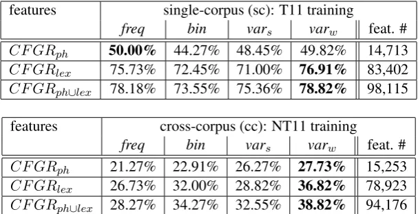
Single- vs. cross-corpus results The results for thethree feature typesusing thefour different feature representationsare presented in Table 1. The chance baseline for the given data setup is 9.1%. There are big accuracy differences between the single- and cross-corpus settings despite very similar feature counts. The drop for the cross-corpus settings is roughly around1

2compared to the single-corpus settings.

This is in line with previous results on the same data sets using a wide range of features (Bykh et al., 2013), confirming the fact that obtaining high cross-corpus results remains challenging in NLI.

features single-corpus (sc): T11 training

freq bin vars varw feat. #

CF GRph 50.00% 44.27% 48.45% 49.82% 14,713

CF GRlex 75.73% 72.45% 71.00% 76.91% 83,402

CF GRph∪lex 78.18% 73.55% 75.36% 78.82% 98,115

features cross-corpus (cc): NT11 training

freq bin vars varw feat. #

CF GRph 21.27% 22.91% 26.27% 27.73% 15,253

CF GRlex 26.73% 32.00% 28.82% 36.82% 78,923

CF GRph∪lex 28.27% 34.27% 32.55% 38.82% 94,176

Table 1: Results for theCF GRfeature variants obtained on the standard T11testset

Best feature type TheCF GRlexfeature type clearly outperforms the more abstractCF GRphfeature

type, yielding up to 28% difference in accuracy for the single-corpus and up to 9% for the cross-corpus settings. In contrast to previous research assuming that lexicalized trees are too topic-specific, the results show thatCF GRlex is a valuable feature type in both the single-corpus and the cross-corpus settings.

TheCF GRlexfeatures combine syntactic and lexical information, such as the fact that a given token with

a particular POS is used, e.g., the tokencanbeing used as anouninThere is acanof beer in the fridge

instead of as the more frequentmodal verbuse inHecandance. Note that this is different from using word and POS unigrams as features, where the relevant connection is lost. In both the T11 data, which is topic balanced, for single-corpus evaluation and the very heterogeneous NT11 data containing a wide range of topics for cross-corpus evaluation, we obtained consistently better results forCF GRlexthan for

CF GRph. Some syntactic rules including lexical information thus seem to generalize well across topics.

CombiningCF GRphandCF GRlexintoCF GRph∪lexgives an additional boost in performance.

Best feature representation There are clear differences in Table 1 between the results for the four feature representations.varwyields the best accuracies in five out of six settings, across different feature

types and corpora.

The results show that WEKA-normalized raw frequencies such as freqyield the worst results in a cross-corpus setting but perform very well single-corpus, which is in line with the assumption that raw frequency features do not generalize well. In our experiments, the performance offreqin a cross-corpus setting is up to 10.55% worse than what is yielded by varw, despite comparable single-corpus

Using binary features (bin) yields better results cross-corpus than freq, whereas in the single-corpus setting it is the other way round. The abstraction introduced by the binary feature representation thus shows a positive effect in terms of the capability of the features to generalize to other data sets.

For the abstractCF GRphfeatures,varsperforms better thanfreqorbinin the cross-corpus setting.

The fact that thevarw is performing consistently better thanvarsshows that weighting is important.

Hence, incorporating the insight from variationist sociolinguistics is not only conceptually interesting as a theoretical perspective, but also provides a quantitative advantage in terms of performance.

CFGR categories as variables As mentioned above, the best performance is achieved by combining

CF GRphandCF GRlexinto theCF GRph∪lexfeature type using the weighted variationist feature

rep-resentationvarw. Thus, we focused on that feature type and explored it more in depth. We did so by

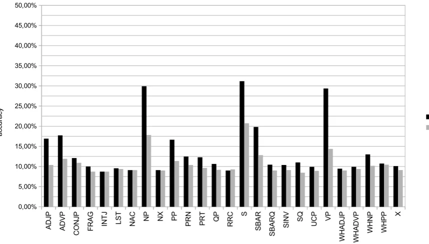
splitting the overallvarwnormalizedCF GRph∪lexfeature set by the variable, i.e., the differentmother nodes. We trained separate models, where each of those models consists of features encoding the differ-ent variants, i.e., the differdiffer-ent realizations in which a given mother node can be rewritten. Our aim was to investigate the accuracy of the individual variable-based models and their contribution to the overall performance. Figures 1 and 2 depict the single-corpus (sc) and cross-corpus (cc) accuracies yielded by each individual variable-based model, for presentation reasons shown separately for theCF GRph and

theCF GRlexsubsets.

A D JP A D V P C O N JP F R A G IN T J LS T N A C N P N X P P P R N P R T Q P R R C S S B A R S B A R Q S IN V S Q U C P V P W H A D JP W H A D V P W H N P W H P P X 0,00% 5,00% 10,00% 15,00% 20,00% 25,00% 30,00% 35,00% 40,00% 45,00% 50,00% sc cc models ac cu ra cy

Figure 1: Accuracy for the individualCF GRphvariable based models,varwnormalized

TheCF GRphresults in Figure 1 show that a small subset of variables performs relatively well. Most

of the models perform poorly, yielding accuracies close to the chance baseline. The best performing variables are essentially the main phrasal categories, such as S, NP, VP, PP, ADJP, ADVP or SBAR.

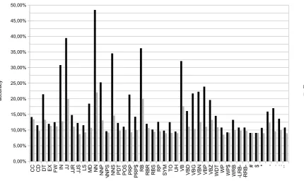
The results for theCF GRlexin Figure 2 show a similar pattern. There is a subset of variables which

perform relatively well, usually models based on the main POS categories, such as the nominal (NN) and verbal (VB) categories as well as adjectives (JJ), prepositions (IN) and adverbs (RB). Some punctuation marks also seem to play a role. The rest of the models yields accuracies around the chance baseline. This might be due to data sparsity given that the main POS categories also are the most frequent. But those main categories also have the highest number of variants through which they can be realized. The good performance of the models for the variables with the highest number of variants thus confirms the assumption that the choice of one of the realization options of a given category is influenced by the L1.

C C C D D T E X F

W IN JJ

JJ R JJ S _LS M D N N N N P N N P S N N S P D T P O S P R P P R P $ R B R B R R B S R P S Y

M _TO

U H V B V B D V B G V B N V B P V B Z W D T W P W P $ W R B -L R B --R R B - # $ '' , . _{: ``} 0,00% 5,00% 10,00% 15,00% 20,00% 25,00% 30,00% 35,00% 40,00% 45,00% 50,00% sc cc models ac cu ra cy

Figure 2: Accuracy for the individualCF GRlexvariable based models,varw normalized

4 Ensemble optimization and tuning

Ensemble generation To combine the individual models, we employ a probability-estimate-based en-semble approach, following Tetreault et al. (2012) and Bykh et al. (2013). This meta-classifier combines the probability distributions provided by the individual classifier for each of the incorporated models as features. To obtain the ensemble training files, we performed 10-fold cross-validation for each model on the corresponding training set and took the probability estimate distributions. For testing, we took the probability estimate distribution yielded by each individual model trained on the corresponding training set and tested on the T11testset. To obtain the probability estimates for the individual models we used LIBLINEAR as described in section 3.2. The ensembles were trained and tested using LIBSVM with an RBF kernel (Chang and Lin, 2011), which outperformed LIBLINEAR for this purpose.

Ensemble optimization (+opt) The growing range of features used for NLI raises the question of how to perform model selection. Even when analyzing a single feature type in depth, as we do in section 3.2, we already must determine which of the low-performing models to keep in an ensemble. We approach the question with a simple incremental ensemble optimization algorithm performing model selection. Algorithm 1Ensemble Optimization / Ensemble Model Selection

Ma← {m1, ..., mn} .overall ensemble, i.e., all ensemble models

Mb ← ∅ .current best performing ensemble

whileMa6=∅do .iterate untilMais empty

mb ←MAX(Ma) .get the model with the highest accuracymbout ofMa

Mt←Mb∪ {mb} .join the previous best performing ensembleMb and{mb}

ifACC(M_t)>ACC(M_b)then .check if the new ensemble is performing better thanM_b

Mb ←Mt .if the accuracy improves, store the new ensemble inMb

end if

REMOVE(m_b, M_a) .removem_bfromM_a

In each iteration step the optimization algorithm shown in Algorithm 1 retrieves the current best single modelmbout of the model setMa(which is initialized with the overall model set for a particular setting),

joins it with the previous best performing ensembleMb(which is initialized to∅), compares the accuracy

of that new ensemble with the accuracy of the previous best ensemble. It retains the new ensemble as the best ensemble if the accuracy improves, or keeps the previous best ensemble as best ensemble otherwise. In Algorithm 1, we describe only the gist of the optimization, omitting some details to keep it transparent. Some ambiguities have to be resolved. If there are several models inMayielding the same accuracy, one

has to decide, which of them to pick as the nextmb. We resolve that issue by always picking the model

with the least number of features. When several models yield the same accuracy and have the same number of features, we resort to alphabetical order. The optimization is always carried out using 10-fold cross-validation results on the training data (to obtain the accuracy ranking onMa and to perform each

optimization step). Thetestset is not part of the optimization at any point. Only after optimization is the resulting ensemble applied to thetestset and we report the corresponding accuracies.

Ensemble tuning (+all) In order to further tune the ensemble, we explore the following idea: We generate asingle ensemble modelmn+1based onallof the features used in a particular setting, i.e., all the

features incorporated by the modelsm1. . . mn. Then we include thatmn+1model in theMaensemble

as just another model, and use that newM+1

a ensemble either directly or as basis for the optimization.

Sincemn+1incorporates all of the features of interest for a particular setting, it is expected to yield more

reliable probability estimates than the other individual ensemble models inM+1

a , each covering only

a subset of that feature set. Incorporating such anmn+1 into the ensemble may stabilize the resulting

system, i.e., the machine learning algorithms may learn to rely onmn+1 in settings, where the rest of

the included modelsm1. . . mnshow a rather poor individual performance and are of limited use. In the

tables and explanations below, we refer to the modelmn+1as [all] and to theMa+1ensemble as+all.

For building the mn+1 model included in the Ma+1 ensemble there are two options. We can build

it on the basis of the probabilities of the models or on the union of the original feature values of those models. In the former case, the final ensemble model essentially is a meta-meta-classifier. For the settings integrating the same type of feature representations (cf. results in Tables 2 and 4), we use the original feature values merged into a single vector to build mn+1. For the settings integrating different feature

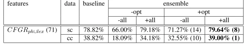
types (cf. results in Table 6), we use the probability estimates from the modelsm1. . . mnto buildmn+1. Ensemble results for the CFGR variables The ensemble results for the separate variable-based mod-els for theCF GRph∪lexfeature type are presented in Table 2. We provide single-corpus (sc) and

cross-corpus (cc) results for different ensemble settings, where+/- optstates whether ensemble optimization was performed, and+/- allwhether tuning was employed. Concretely,(-opt, -all)means that the ensem-bleMawas used without any optimization or tuning, and correspondingly(+opt, +all)means that the

optimized and tuned version ofMa(i.e., the optimized version of the ensembleMa+1) was employed. In

the remaining two cases(+opt, -all)and(-opt, +all)either optimization or tuning was used, respectively. The columnbaselinelists the corresponding results from Table 1, which were obtained by putting all the features in a single vector. The number in parentheses specifies the number of models combined in the ensemble: in thefeaturescolumn, it shows the overall number of separate variable-based models, and in the+optcolumns, it is the number of models selected by the optimization algorithm.

features data baseline ensemble

-opt +opt

-all +all -all +all

CF GRph∪lex(71) sc 78.82% 66.00% 79.18% 71.27% (14) 79.64% (8)

cc 38.82% 18.09% 34.18% 32.55% (10) 39.00% (1) Table 2: Results for theCF GRph∪lexensembles with different optimization settings

the drop in the cross-corpus setting is more than 20% is particularly striking. We assume that this is due to the poor performance of most of the individual models, yielding probabilities of little use overall. The few relatively well-performing models we discussed in section 3.2 apparently are flooded by the noise introduced by the others. Thus, for a set of rather low-performing models without any optimization, it seems preferable to provide the classifier with access to the individual features instead of to the noisy probability estimates. The optimization(+opt, -all)leads to a clear improvement over the non-optimized settings. In the single-corpus setting only 14 of the 71 models were kept and in cross-corpus only 10.

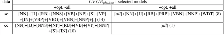
Table 3 shows the selected models in the order in which they are selected by the ensemble optimization algorithm. For(+opt, -all), the table basically consists of the best performing variables (i.e., the models containing as features the different ways to rewrite the given mother category) as discussed in section 3.2, suggesting that the algorithm makes meaningful choices.

data CF GRph∪lex: selected models

+opt, -all +opt, +all

sc [NN]+[JJ]+[RB]+[NNS]+[VB]+[NP]+[S]+[VP] [all]+[NN]+[JJ]+[RB]+[PRP]+[VBN]+[NNP]+[WDT] (8) +[IN]+[VBP]+[VBG]+[VBN]+[NNP]+[,] (14)

cc [NN]+[JJ]+[NNS]+[NP]+[RB]+[VB]+[VP]+[NNP] [all] (1) +[S]+[IN] (10)

Table 3: TheCF GRph∪lexmodel sets selected by optimization

The flipside of the coin is that low-performing models generally were not found to have a positive effect and thus were not included. Yet, optimization by itself is not successful overall given that the

(+opt, -all)accuracy remains below the single feature set baseline.

Applying tuning without optimization(-opt, +all)outperforms the optimization result. Thus, includ-ing the overall model [all] in the ensemble improves the meta-classifier. In the single-corpus setting, the accuracy is slightly higher than the baseline, in cross-corpus it remains below the baseline.

Turning on both optimization and tuning(+opt, +all)yields the overall best results of Table 2, 79.64% for single-corpus and 39% for the cross-corpus setting. The corresponding entry in Table 3 shows that tuning significantly reduces the number of selected models. This is not unexpected given that the overall model [all] essentially includes all the information. In the cross-corpus setting, [all] indeed is the only model selected. Interestingly, in the single-corpus setting, the optimization algorithm identifies some additional models to improve the accuracy, mainly ones that also perform well individually. While this amounts to adding information that in principle is already available to the [all] model, the improvement may stem from the abstract nature of the probability estimates used as features of the meta-classifier. When both optimization and tuning are applied, the tuning apparently stabilizes the ensemble leading to higher performance, and the optimization algorithm further improves the result by reducing the noise.

5 Combining CFGR with four types of n-grams

Based on the systematic exploration of the CFGR domain, we turn to combining our new feature type

CF GRph∪lexwith n-gram features as the best performing features for NLI (Tetreault et al., 2013; Jarvis

et al., 2013). Adapting the n-gram approach we presented in Bykh and Meurers (2012), we use all recurring n-grams with1≤n≤10at different levels of representation, including the word-based (W), open-class POS-based (OP) and POS-based (P) n-grams from our previous work as well as lemma-based (L) n-grams (Jarvis et al., 2013). We employ binary feature encoding for all n-gram types.

For POS-tagging we use the OpenNLP1 _{toolkit, for lemmatizing we employ the MATE}2 _tools (Bj¨orkelund et al., 2010). To obtain a fine grained, flexible n-gram setting, we generate an ensemble model for each n-gram type and eachn, which results in 40 n-gram models.

1_{http://opennlp.apache.org}

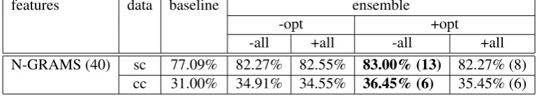
Table 4 provides the results for the n-gram ensembles built on the basis of the recurring word-, lemma-, POS-, OCPOS-based n-grams with 1 ≤ n ≤ 10 in the same format as Table 2 for CF GRph∪lex.3

Different from theCF GRph∪lexcase, the results for the n-gram ensemble model without optimization

or tuning(-opt, -all)already are 4–5% higher than the single vector baseline. features data baseline ensemble

-opt +opt

-all +all -all +all N-GRAMS (40) sc 77.09% 82.27% 82.55% 83.00% (13) 82.27% (8)

cc 31.00% 34.91% 34.55% 36.45% (6) 35.45% (6) Table 4: Results for the n-gram ensembles with different optimization settings

The best results, 83% for single-corpus and 36.45% for the cross-corpus setting, are obtained by ap-plying the optimization. The n-gram ensembles seem to benefit more from optimization than from tuning in general. The feature counts for the n-grams (single-corpus: 4,822,874; cross-corpus: 3,687,375) are far higher than forCF GRph∪lex (single-corpus: 98,115; cross-corpus: 94,176), so there may be more

noise in the [all] model, making it less useful for the tuning step.

Table 5 lists the models selected by the optimization algorithm in order in which they are selected. The n-gram types and thenof the model is indicated, e.g., “[OP-3]” means “OCPOS-based trigrams”.

data N-GRAMS: selected models

+opt, -all +opt, +all

sc [W-2]+[L-2]+[W-1]+[L-1]+[L-3]+[W-3]+[OP-3] [all]+[W-2]+[L-2]+[W-1]+[L-1]+[L-3]+[OP-4]+[L-4] (8) +[OP-1]+[OP-5]+[P-3]+[P-5]+[P-2]+[OP-8] (13)

cc [W-2]+[W-1]+[L-1]+[L-3]+[W-3]+[OP-2] (6) [W-2]+[W-1]+[all]+[L-1]+[L-3]+[P-4] (6)

Table 5: The n-gram model sets selected by optimization

For the more surface-based n-gram (word- and lemma-based), the optimizer selected only up ton= 3, whereas for the more abstract ones (POS- and OCPOS-based), models up ton= 8were included. Thus, when abstracting from the surface, one can get some useful information out of longer n-grams that apparently is not contained in the short surface-based ones. Different from theCF GRph∪lex

variables-based ensemble, we here find that relatively low-performing models such as those considering longern

n-grams are kept when optimizing the ensemble.

Having established the performance of the n-gram ensembles, we can turn to combining the

CF GRph∪lexand n-gram models. The results are presented in Table 6.

features data ensemble

-opt +opt

-all +all -all +all

(a)CF GRph∪lex(71) + N-GRAMS (40) sc 82.09% 82.91% 82.91% (20) 83.55% (6)

cc 34.09% 36.00% 36.73% (8) 38.45% (3)

(b)CF GRph∪lex(71) + N-GRAMS[+opt, -all](ME) sc 83.09% 83.73% 82.64% (4) 84.18% (5)

cc 37.36% 39.55% 38.00% (3) 40.27% (3)

(c)CF GRph∪lex[+opt, +all](ME) + N-GRAMS (40) sc 83.73% 84.82% 84.73% (13) 83.82% (13)

cc 36.82% 38.91% 42.00% (5) 43.00%(4) (d)CF GRph∪lex[+opt, +all](ME) + N-GRAMS[+opt, -all](ME) sc 83.45% 83.45% 83.45% (2) 83.36% (2)

cc 41.27% 42.00% 41.27% (2) 40.55% (2)

Table 6: Optimization results combining n-grams andCF GRph∪lex

3_{For space reasons, we cannot present the individual results for the separate n-gram models here, but interested readers}

We explore four different ways to combine the two model sets, and the table shows the best results for each of the setups in bold, once for the single-corpus and once for the cross-corpus setting.

For the results of setup (a), we use the ensemble consisting of all individual models separately. In (b), theCF GRph∪lexmodels are included as in (a), but we replace the n-gram models by asingle meta-ensemble model (ME)generated using the best n-grams setting (+opt, -all), which consists of 13 models for single-corpus and six models for the cross-corpus setting (see Table 4). ME thus is a meta-meta-classifier, generated by applying the ensemble model generation routine to an ensemble.

In (c), we invert the (b) setting: TheCF GRph∪lexfeatures are replaced by a meta-ensemble generated

using the best performing CF GRph∪lex setting (+opt, +all), which consists of eight models for the

single-corpus, and one model for the cross-corpus setting (see Table 2).

Finally, in (d) we combine the meta-ensemble for CF GRph∪lex with the meta-ensemble for the

n-grams obtaining an ensemble consisting of two models

The best results of 84.82% in the single-corpus setting and 43% cross-corpus, underlined in the table, are obtained in setup (c). These are the overall best results across all experiments described in this paper. The best result in the single-corpus setting involves tuning only, whereas in the cross-corpus setting it involves tuning and optimization selecting the models [all]+[CFGR +all +opt]+[W-2]+[W-1].

The single-corpus accuracy of 84.82% is the best result reported so far for the NLI Shared Task 2013 data with the T11train∪dev set for training and the T11testset for testing. The best previous result was 83.6% (Jarvis et al., 2013).

In the cross-corpus setting, the 43% accuracy also outperforms the previous best result on the NT11 data (Bykh et al., 2013) by 4.5%.

In sum, the overall best results in the single-corpus and cross-corpus settings are obtained starting with the whole n-gram model set plus an optimizedCF GRph∪lex meta-ensemble. This confirms the

useful-ness of the optimized ensemble setup and underlines that combining a range of linguistic properties, from n-grams at different levels of abstraction to local syntactic trees characteristics, is a particularly fruitful approach for native language identification as a good example of an experimental task putting linguistic modeling to the test with real-life data.

6 Conclusions

In the research presented, we systematically explorednon-lexicalizedandlexicalized CFG production rules (CFGR)as features for the task of NLI using both single-corpus and cross-corpus settings. Includ-ing lexicalized CFG rule features clearly improved the results in both settInclud-ing so that it seems worthwhile not to discard them a priori, which was the standard in previous research.

Pursuing avariationist perspectiveto CFGR feature representation resulted in improved performance and it supported an in-depth exploration of the contribution of the different variables and variants as well as of the value of local syntactic features for NLI in general. Training a separate classifier for each variable provides quantitative advantages by facilitating high-performing ensemble setups and supports a qualitative discussion of the categories reflecting the choices made by the learners with a given L1.

Investigating different meta-classifier setups, we explored ensemble optimization and tuning tech-niques that improved the accuracy over putting all features in a single vector or a basic ensemble setup.

Combining the syntactic CFGR with four types of n-grams yielded asingle-corpusaccuracy of84.82%

on the TOEFL11testset. To the best of our knowledge this is the highest accuracy reported so far on this standard data set of the NLI Shared Task 2013. The combined model also outperformed our best previous cross-corpus result on the NT11 corpus.

References

Anders Bj¨orkelund, Bernd Bohnet, Love Hafdell, and Pierre Nugues. 2010. A high-performance syntactic and semantic dependency parser. InDemonstration Volume of the 23rd International Conference on Computational Linguistics (COLING 2010), Beijing, pages 23–27.https://code.google.com/p/mate-tools/. Daniel Blanchard, Joel Tetreault, Derrick Higgins, Aoife Cahill, and Martin Chodorow. 2013. TOEFL11: A

corpus of non-native english. Technical report, Educational Testing Service.

Julian Brooke and Graeme Hirst. 2012. Robust, lexicalized native language identification. InProceedings of the 24th International Conference on Computational Linguistics (COLING), pages 391–408, Mumbai, India. Julian Brooke and Graeme Hirst. 2013a. Native language detection with ’cheap’ learner corpora. In Sylviane

Granger, Ga¨etanelle Gilquin, and Fanny Meunier, editors,Twenty Years of Learner Corpus Research. Looking Back, Moving Ahead. Proceedings of the First Learner Corpus Research Conference (LCR 2011), Louvain-la-Neuve, Belgium. Presses universitaires de Louvain.

Julian Brooke and Graeme Hirst. 2013b. Using other learner corpora in the 2013 nli shared task. InProceedings of the 8th Workshop on Innovative Use of NLP for Building Educational Applications (BEA-8) at NAACL-HLT 2013, Atlanta, GA.

Serhiy Bykh and Detmar Meurers. 2012. Native language identification using recurring n-grams – investigating abstraction and domain dependence. In Proceedings of the 24th International Conference on Computational Linguistics (COLING), pages 425–440, Mumbay, India.

Serhiy Bykh, Sowmya Vajjala, Julia Krivanek, and Detmar Meurers. 2013. Combining shallow and linguistically motivated features in native language identification. InProceedings of the 8th Workshop on Innovative Use of NLP for Building Educational Applications (BEA-8) at NAACL-HLT 2013, Atlanta, GA.

Chih-Chung Chang and Chih-Jen Lin. 2011. LIBSVM: A library for support vector machines. ACM Transactions on Intelligent Systems and Technology, 2:27:1–27:27. Software available athttp://www.csie.ntu.edu. tw/˜cjlin/libsvm.

Andrea Cimino, Felice Dell’Orletta, Giulia Venturi, and Simonetta Montemagni. 2013. Linguistic profiling based on general–purpose features and native language identification. InProceedings of the 8th Workshop on Innova-tive Use of NLP for Building Educational Applications (BEA-8) at NAACL-HLT 2013, Atlanta, GA.

R.E. Fan, K.W. Chang, C.J. Hsieh, X.R. Wang, and C.J. Lin. 2008. Liblinear: A library for large linear classification. The Journal of Machine Learning Research, 9:1871–1874. Software available at http: //www.csie.ntu.edu.tw/˜cjlin/liblinear.

Binyam Gebrekidan Gebre, Marcos Zampieri, Peter Wittenburg, and Tom Heskes. 2013. Improving native lan-guage identification with tf-idf weighting. InProceedings of the 8th Workshop on Innovative Use of NLP for Building Educational Applications (BEA-8) at NAACL-HLT 2013, Atlanta, GA.

S. Granger, E. Dagneaux, and F. Meunier. 2002. International Corpus of Learner English. Presses Universitaires de Louvain, Louvain-la-Neuve.

Sylviane Granger, Estelle Dagneaux, Fanny Meunier, and Magali Paquot, 2009. International Corpus of Learner English, Version 2. Presses Universitaires de Louvain, Louvain-la-Neuve.

Mark Hall, Eibe Frank, Geoffrey Holmes, Bernhard Pfahringer, Peter Reutemann, and Ian H. Witten. 2009. The weka data mining software: An update. InThe SIGKDD Explorations, volume 11, pages 10–18.

Shin’ichiro Ishikawa. 2011. A new horizon in learner corpus studies: The aim of the ICNALE projects. In G. Weir, S. Ishikawa, and K. Poonpon, editors,Corpora and language technologies in teaching, learning and research, pages 3–11. University of Strathclyde Publishing, Glasgow, UK. http://language.sakura. ne.jp/icnale/index.html.

Scott Jarvis and Scott A. Crossley, editors. 2012. Approaching Language Transfer through Text Classification: Explorations in the Detection-based Approach. Second Language Acquisition. Multilingual Matters.

Scott Jarvis, Yves Bestgen, and Steve Pepper. 2013. Maximizing classification accuracy in native language iden-tification. InProceedings of the 8th Workshop on Innovative Use of NLP for Building Educational Applications (BEA-8) at NAACL-HLT 2013, Atlanta, GA.

Moshe Koppel, Jonathan Schler, and Kfir Zigdon. 2005. Determining an author’s native language by mining a text for errors. InProceedings of the eleventh ACM SIGKDD international conference on Knowledge discovery in data mining (KDD ’05), pages 624–628, New York.

William Labov. 1972.Sociolinguistic Patterns. University of Pennsylvania Press.

Andr´e Lynum. 2013. Native language identification using large scale lexical features. In Proceedings of the 8th Workshop on Innovative Use of NLP for Building Educational Applications (BEA-8) at NAACL-HLT 2013, Atlanta, GA.

Shervin Malmasi, Sze-Meng Jojo Wong, and Mark Dras. 2013. Nli shared task 2013: Mq submission. In Proceedings of the 8th Workshop on Innovative Use of NLP for Building Educational Applications (BEA-8) at NAACL-HLT 2013, Atlanta, GA.

Detmar Meurers, Julia Krivanek, and Serhiy Bykh. 2013. On the automatic analysis of learner corpora: Native language identification as experimental testbed of language modeling between surface features and linguistic abstraction. InDiachrony and Synchrony in English Corpus Studies, Frankfurt am Main. Peter Lang.

Mick Randall and Nicholas Groom. 2009. The BUiD Arab learner corpus: a resource for studying the acquisition of L2 english spelling. InProceedings of the Corpus Linguistics Conference (CL), Liverpool, UK.

Benjamin Swanson and Eugene Charniak. 2012. Native language detection with tree substitution grammars. In Proceedings of the 50th Annual Meeting of the Association for Computational Linguistics (Volume 2: Short Papers), pages 193–197, Jeju Island, Korea, July. Association for Computational Linguistics.

Ben Swanson and Eugene Charniak. 2013. Extracting the native language signal for second language acquisition. InProceedings of NAACL-HLT. Association for Computational Linguistics.

Ben Swanson. 2013. Exploring syntactic representations for native language identification. InProceedings of the 8th Workshop on Innovative Use of NLP for Building Educational Applications (BEA-8) at NAACL-HLT 2013, Atlanta, GA.

Sali A. Tagliamonte. 2011. Variationist Sociolinguistics: Change, Observation, Interpretation. John Wiley & Sons.

Joel Tetreault, Daniel Blanchard, Aoife Cahill, and Martin Chodorow. 2012. Native tongues, lost and found: Resources and empirical evaluations in native language identification. InProceedings of the 24th International Conference on Computational Linguistics (COLING), pages 2585–2602, Mumbai, India.

Joel Tetreault, Daniel Blanchard, and Aoife Cahill. 2013. A report on the first native language identification shared task. InProceedings of the Eighth Workshop on Building Educational Applications Using NLP, Atlanta, GA, USA, June. Association for Computational Linguistics.

Sze-Meng Jojo Wong and Mark Dras. 2011. Exploiting parse structures for native language identification. In Proceedings of the 2011 Conference on Empirical Methods in Natural Language Processing, pages 1600–1610, Edinburgh, Scotland, UK., July.