ESTIMATING THE TRUE PERFORMANCE OF CLASSIFICATION-BASED NLP T E C H N O L O G Y
James R. Nolan Siena College Loudonville, NY 12211
Abstract
Many of the tasks associated with natural language processing (NLP) can be viewed as classification problems. Examples are the computer grading of student writing samples and speech recognition systems. If we accept this view, then the objective of learning classifications from sample text is to classify and predict successfully on new text. While success in the marketplace can be said to be the ultimate test of validation for NLP systems, this success is not likely to be achieved unless appropriate techniques are used to validate the prototype. This paper discusses useful validation techniques for classification-based NLP systems and how these techniques may be used to estimate the true performance of the system.
INTRODUCTION
The objective of learning classifications from sample text is to classify and predict successfidly on new text. For example, in developing a system for grading student writing samples, the objective is to learn how to classify student writing samples into grade categories so that we may use the system to predict successfully the grade categories for new samples of student writing (Nolan, 1997a).
The most commonly used measure of success or failure is a classifier's error rate (Weiss & Kulikowski, 1991). Each .time the classifier is presented with a case, it makes a decision about the appropriate class for the case. Sometimes it is right; sometimes it is wrong. The true error rate is statistically defined as the error rate of the classifier on a large number of new cases that converge in the limit to the actual population distribution.
I f we were given an unlimited number o f cases, the true error rate could be readily computed as the number of samples approached infinity. In the real world, the number of
samples is always finite, and typically relatively small. The major question is then whether it is possible to extrapolate from empirical error rates calculated from small sample results to the true error rate. It turns out that there are a number of ways of presenting sample cases to a classifier to get better estimates of the true error rate. Some of these techniques are better than others. In statistical terms, some estimators of the true error rate are considered biased. They tend to estimate too low, i.e., on the optimistic side, or too high, i.e., on the pessimistic side.
In the next section, we will define just what an error is when using classification systems for natural language processing. The apparent error rate will be contrasted with the true error rate. The effect of classifier complexity and feature dimensionality on classification results will be followed by conclusions.
WHAT IS AN ERROR?
An error is simply a misclassification: the classifier is presented a case, and it classifies the case incorrectly. If all errors are of equal importance, a single error rate, calculated as follows,
number of errors error rate --
number of cases
healthy person without any permanent damage (except possibly to one's pocket book), whereas an illness left untreated will probably get worse and lead to more serious problems, even death. Although not usually a life and death decision, classifying a student's writing sample can result in the same type of false negative and false positive errors.
Let us suppose the writing sample evaluation is being made to help determine whether the student will be placed into a program designed to help poor writers to improve their writing skills. In this case, as in the previous one, there are two errors that can be made. The evaluation of the writing sample could indicate that the student should not need to be placed in the special writing program when in fact they are deficient in writing skills (a false negative). Or the evaluation could indicate that the student shouM be placed in the special writing program when the student's writing skills are really at a level indicating he or she does not need extra help (false positive).
The question is whether the two types of errors committed in the writing sample evaluation scenario - false negative and false positive errors, respectively - are of the same consequence. If they are not, then we must extend our definition of error.
Costs and Risks
A natural alternative to an error rate as previously defined is a misclassification cost (lVlachina, 1987). Here, instead of designing a classifier to minimize error rates, the goal would be to minimize misclassification costs. A misclassification cost is simply a number that is assigned as a penalty for making a mistake. For example, in the two-class situation, a cost of one might be assigned to a false positive error and a cost of two to a false negative error. An average cost of misclassitication can be obtained by weighing each of the costs by the respective error rate. Computation,ally, this means that the errors are converted into costs by multiplying an error by its misclassification cost. The effect of having false negatives cost twice what false positives cost will be to tolerate many more false positive errors than false negative ones for a fixed classifier design. If an optimal decision- making strategy is followed, cost choices have a direct effect on decision thresholds and resulting error rates.
If we assign a cost to each type of error or misclassification, the total cost of misclassification is most directly computed as the sum of the costs for each error. If all misclassifications are assigned a cost of 1, the total cost is given by the number of errors, and the average cost per decision is the error rate. By raising or lowering the cost of misclassification, we are biasing decisions in different directions, as if there were more or fewer cases in a given class. Formally, ff i is the predicted class and j is the true class, then for n classes, the total cost of misclassification is
n n
Cost = Z E Eij Cij i = l j = l
where Eq is the number of errors and Cq is the cost for that type misclassification. O f course, the cost of a correct classification (Cq, for i=j) is 0.
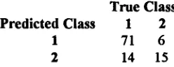
For example, using the data in Figure 1, ff the cost of misclassifying a class 1 case is 1, and the cost of miselassifying a class 2 case is 2, then the total cost of the classifier is (14 * 1) + (6 * 2) = 26 and the average cost per decision is 26/106 = .25. This is quite different from the result if costs had been equal and set to 1, which would have yielded a total cost of merely 20, and an average cost per decision of .19 (Weiss & Kulikowski, 1991).
True Class Predicted Class 1 2
1 71 6
2 14 15
Figure 1: Sample Classification Results We have so far considered the costs of misclassifications, but not the potential for expected gains arising from correct classification. In risk armlysis or decision analysis, both costs (or losses) and benefits (gains) are used to evaluate the performance of a classifier. A rational objective of the classifier is to maximize gains. The expected gain or loss is the difference between the gains for correct classifications and losses for incorrect classifications.
[image:2.612.364.488.478.526.2]assigned as negative numbers, and gains from correct classification as positive numbers, then we can express the total risk as
n n
Risk = g g E~jR~
i=l j=lwhere Eq is once again the number of errors and R e is the risk of classifying a case that truly belongs in class j into class i.
Costs and risks can all be employed in conjunction with error rate analysis. In some ways, they can be viewed as modified error rates. If conventionally agreed upon units, such as monetary costs, are available to measure the value of a quantity, then a good case can be made for the usefulness of basing a decision system on these alternatives as opposed to one based directly on error rates. The implication for classification-based NLP is that attention must be paid to the context o f the particular application as regards the costs and risks associated with the possible errors in classification.
APPARENT VS. TRUE ERROR RATE
As stated earlier, the true error rate of a classifier is defined as the error rate of the classifier ff it was tested on the true distribution of cases in the population - which can be empirically approximated by a very large number of new cases gathered independently from the cases used to design the classifier.
The apparent error rate of a classifier is the error rate of the classifier on the sample cases that were used to design or build the system. In general, the apparent error rates tend to be biased optimistically. The true error rate is almost invariably higher than the apparent error rate. This happens when the classifier has been overfitted (or overspecialized) to the particular characteristics of the sample data (Ripley,
1996).
It is useless to design a classifier that does well on the design sample, but does poorly on new cases. And unfortunately, as just mentioned, using solely the apparent error to estimate future performance can often lead to disastrous results on new data. To illustrate this, we can look at an example from speech recognition. Any novice could design a classifier with a zero apparent error rate simply by using a
direct table lookup approach as illustrated in Figure 2. A sample of one individual's speech and pronunciation patterns become the classifier. When trying to interpret a spoken word from this individual, we would just lookup the answer (classification) in the table containing their speech patterns.
If we test on the original speech data, and no pattern is repeated for different classes, we never make a mistake. Unfortunately, when we bring in new speech data (another person's speech), the odds of finding the individual case in the aforementioned table are extremely remote because of the enormous number of possible combinations of speech features.
~
Decision by [
Table Lookup[ ~
of Original ]~q-"lCases I
Samples
IFigure 2: Classification by Table Lookup
The nature of this problem, which is illustrated most easily with the table lookup approach, is caused by overfitting the speech classifier to the data. Basing our estimate of performance of this classifier on the apparent error rate leads to similar problems. While the table lookup is an extreme example, the extent to which classification methods arc susceptible to overfitting varies. Many a learning system designer has been lulled into a false sense of security by the mirage of low apparent error rates.
This problem is of particular concern when analyzing student writing samples where the odds of finding a writing sample identical to one in the test sample are extremely remote because of the enormous number of possible combinations of writing features.
Fortunately, there are very effective techniques for guaranteeing good properties in the estimates of a true error rate even for a small sample. While these techniques can measure the performance of a classifier, they do not guarantee that the apparent error rate is close to the true error rate for a given application.
concept of randomness is very important in obtaining a good estimate of the true error rate. A computer classifieation-based NLP system is always at the mercy of the design samples supplied to it. Without a random sample, the error rate estimates can be compromised, or alternatively, they will apply to a different population than intended.
Train and Test Error Rate Estimation
Many researchers have employed the train-and- test paradigm for estimating the true error rate (Nolan, 1997b). This involves splitting the sample into two groups. One group is called the training set and the other the testing set. The
training
set is used to design the classifier, and the testing set is used strictly for testing. If we "hide" or "hold out" the test cases and only look at them after the classifier design is complete, then we have a direct procedural correspondence to the task of determining the error rate on new cases. The error rate of the classifier on the test cases is called the test sample error rate.As usual, the two sets of cases should be random samples from some population. In addition, the case.s in the two sample sets should be independent. By independent, we mean that there is no relationship among them other than that they are samples from the same population. To ensure that they are independent, they might be gathered at different times or by different researchers.
A question that arises with the train- and-test error rate estimation technique can be stated as: "How many test cases are needed for the test sample error rate to be essentially the true error rate?" The answer is: a surprisingly small number. Moreover, based on the test sample size, we know how far off the test sample estimate can be. These estimations can be derived from basic probability theory. Specifically, the accuracy of error rate estimates for a specific classifier on independent and randomly drawn test samples is governed by the binomial distribution. While a demonstration of the use of the binomial distribution is not shown here, it should be emphasized that the quality of the test sample estimate is directly dependent on the number of test cases. When the test sample size reaches 1000, the estimates are extremely accurate. At sample size 5000, the test sample estimate is virtually identical to the true error rate.
Random Resampling
A single random partition of the data set can be misleading for small or moderately sized samples. In such cases, multiple train-and-test experiments can do better. When multiple train- and-test experiments are performed, a new classifier is learned from each training sample. The estimatod error rate is the average of the error rates for classifiers derived for the independently and randomly generated tests partitions. Random subsampling can produce better error estimates than a single train-and-test partition.
A special case of resampling is known as leaving-one-out (Lachenbruch & Mickey, 1968). For a given method and sample size, n, a classifier is generated using (n-l) cases and tested on the remaining case. This is repeated n times, each time designing a classifier by leaving-one-out. Thus each ease in the sample is used as a test case, and each time nearly all eases are used to design a classifier. The error rate is the number of errors on the single test cases divided by n.
Leaving-one-out is an elegant and straightforward technique for estimating classifier error rates. The leaving-one-out estimator is an almost unbiased estimator of the true error rate of a classifier. This means that over many different sample sets of size n, the leaving-one-out estimate will average out to the true error rate. Suppose you are given 100 sample sets of 50 eases each. The average of the leaving-one-out estimates for each of the 100 sample sets will be very close to the true error rate. Because the leaving-one-out estimator is unbiased, for even modest sample sizes of over
100, the estimate should be accurate.
The great advantage of tlus technique is that all the cases in the available sample are used for testing, and almost all the cases are also used for training the classifier. In addition, much smaller sample sizes than those required in the train-test method can lead to very accurate estimation. There is an increased computational cost, however.
Bootstrapping
difficulties with this technique. Both the bias and variance of an error estimator contribute to the inaccuracy and imprecision of the error rate estimate. While leafing-one.out is nearly unbiased, its variance is high for small samples.
A more recently discovered resampling method, called bootstrapping, has shown much promise as an error rate estimator (Efron, 1983). There are numerous bootstrap estimators. We will discuss one, called the e0 bootstrap estimator. For this, a training group consists of n cases sampled with replacement from a size n sample. Sampled with replacement means that the training samples are drawn from the data set and placed back after they are used, so their repeated use is allowed. Cases not found in the training group form the test group. The estimated error rate is the average of the error rates over a number of iterations. About 200 iterations for bootstrap estimates are considered necessary to obtain a good estimate. Thus, this is computationally considerably more expensive than leaving-one-out.
CLASSIFIER COMPLEXITY AND FEATURE DIMENSIONALITY Intuitively, one expects that the more information that is available, the better one should do. The more knowledge we have, the better we can make decisions. Similarly, one might expect that a theoretically more powerful
classification method should work better in
practice. Surprisingly, in practice, both of these expectations are wrong (Wallace & Freeman,
1987).
Most classification methods involve
compromises. They make some assumptions
about the population distribution and about the decision process fitting a specific type of representation. The samples, however, are often treated as a somewhat mysterious collection. The features thought to differentiate the object classes have been preselected (hopefully by an experienced person), but initiaily it is not known whether they are high quality features or whether they arc highly noisy or redundant. If the features all have good predictive capabilities, any one of many classification methods should do well. Otherwise, the situation is much less predictable.
Suppose one is trying to make an evaluation about the level of reading
comprehension understanding exhibited in a sample piece of student writing based on five features. Later two new features are added and samples collected. Although no data has been deleted, and new information has been added, some methods may actually yield worse results on the new, more complete set of data than on the original, smaller set. These results can be reflected in poorer apparent error rates, but more often in worse (estimated) true error rates. What
causes this phenomenon of performance
degradation with additional information? Some methods perform particularly well with good, highly predictive features, but fail apart with noisy data. Other methods may overweight redundant features that measure the same thing by, in effect, counting them more than once.
In practice, many features used in NLP applications are often poor, noisy, and redundant. Adding new information in the form of weak features can actually degrade performance of the system. This is particularly true of methods that are applied directly to the data without any estimate of complexity fit to the data. For these methods, the primary approach to minimize the effects of feature noise and redundancy is feature selection. Given some initial set of features, a feature selection procedure will throw out some of the features that are deemed to be noncontributory to classification.
Our goal is to fit a classification model to the data without overspecializing the learning system to the data. Thus, we must determine just how complex a classifier the data supports. In general, we do not know the answer to this question until we estimate the true error rate for different classifiers and classifier fits. In practice, though, simpler classifiers often do better than more complex or theoretically advantageous classifiers. For some classifiers, the underlying assumptions of the more complex classifier may be violated. For most classifiers, the data are not strong enough to generalize beyond an indicated level of complexity fit. As a rule o f thumb, one is looking for the simplest solution that yields good results.
CONCLUSIONS AND RECOMMENDATIONS
the size of the training sample. Irrespective of the classification method, the performance of a classification-based NLP system should be evaluated by estimating the accuracy of future predictions, technically known as estimating the true error rate on future cases. This is of fundamental importance for comparing classifiers on the same samples and also for selecting key characteristics of many of the newer classifiers, e.g., neural networks.
It has been shown that, with limited samples, the best techniques for measuring the performance of classification-based NLP systems are resampling methods that simulate the presentation of new cases by repeatedly hiding some test cases. Additionally, attention must be paid to the context of the particular NLP application as regards the costs and risks associated with the possible errors in classification.
Although statistically valid estimates of the true error rate will not guarantee success in the marketplace for NLP systems, they will give one a measure of confidence in the true performance of the system.
References
Effron, B. (1983). Estimating the Error Rate of a Prediction Rule.
Journal of the American
Statistical Association,
78:316-333.Lachenbruch, P. and Mickey, M. (1968). Estimation of Error Rates in Discriminant Analysis.
Technometrics,
10:1-11.Nolan, James R. (1997a). The Architecture of a Hybrid Knowledge-Based System for Evaluating Writing Samples. In A Niku-Lari (Ed.),
Expert Systems Applications and
Artificial Intelligence Technology Transj~r
Series,
EXPERSYS-97. Gournay s/M,France: IITr International, in press.
Nolan, James R. (1997b). DISXPERT: A Rule- Based Vocational Rehabilitation Risk Assessment System.
Expert Systems With
Applications,
in press.Machina, M. (1987). Decision-Making in the Presence of Risk.
Science,
236: 537-543. Riplcy, Brian D. (1996).Pattern Recognition
and
Neural
Networks.
Cambridge:Cambridge University Press.
Wallace, C. & Freeman, P. (1987). Estimation and Inference by Compact Encoding.