Application of House Holder and Inverse Power Methods of Numerical Methods in MAGDM Problems

(1)

Application of House Holder and Inverse Power

Methods of Numerical Methods in MAGDM

Problems

John Robinson P

1

, Susai Alexander P

2 Assistant Professor1,2

Department of Mathematics, Bishop Heber College, Tiruchirappalli, India.

Department of Mathematics, Loyola College, Vettavalam, India. [email protected]1, [email protected]2

Abstract- The aim of this paper is to investigate the Multiple Attribute Group Decision Making (MAGDM) problems with intuitionistic fuzzy sets. Some numerical methods like House-Holder and Inverse power methods are coupled with linear programming methods for determining the unknown decision maker weights and it is applied in decision making problem. Feasibility and effectiveness of the proposed methods are illustrated using numerical examples.

Key words: Intuitionistic Fuzzy Set, IFWA and IFHA operator, House Holder and Inverse Power method, Linear Programming Method.

1. INTRODUCTION

Multi Attribute Group Decision Making (MAGDM) problems are wide spread in real life situations. It is obvious that much knowledge in the real world is fuzzy rather than precise.Intuitionistic fuzzy set (IFS) Atanassov, (1999) characterized by a membership function and a non-membership function, is an extension of Zadeh’s fuzzy set Zadeh, (1965; 1978; 1983) whose basic components is only a membership function. An IF has been proven to be highly useful to deal with uncertainty and vagueness. Xu, (2007) defined some new intuitionistic preference relations, such as the consistent intuitionistic preference relation, incomplete intuitionistic preference relation and acceptable intuitionistic preference relation, and studied their properties. Gerstenkorn, &Manko, (1991), Robinson &Amirtharaj, (2014; 2015) propose correlation coefficients for different higher order intuitionistic fuzzy sets and utilized them in ranking the alternatives in MAGDM problems. Yager, (2004), Wei et al., (2011) contributed novel approaches to the field of fuzzy decision making. Jain et al. (2006) discussed several numerical methods for scientific and engineering computation. Here, Householder’s and Power method are used to obtain the solution of linear algebraic equation, which are further utilized to derive the decision maker weights in intuitionistic fuzzy decision making problems. The feasibility and effectiveness of

the proposed method are illustrated using numerical examples.

2. PRELIMINARIES

In this section, some basic definitions and intuitionistic fuzzy weighted averaging operator are presented.

Definition 1:Intuitionistic Fuzzy Set

An IFS A in X is given by



,

_A

( ),

_A

( )



,

A



x



x



x



X

where

 

:

0,1

A

X





,



_A

:

X



 

0,1

, with the condition

0





_A

( )

x





_A

( ) 1,

x



 

x

X

.The numbers



_A

 

x

and



_A

 

x

represent, the membership degree and non-membership degree of the element x to the set A, respectively.

Definition 2:For each IFS A in X, if

 

1

 

,

A

x

A

x

A

x

X



 







 

then

 

A

x



is called the degree of indeterminacy of x to A, where 0 ≤



_A

 

x



1

, for all xX.

Definition 3: Let

a

_j





 

_j

,

_j



,

for all j = 1, 2, …,n be a collection of intuitionistic fuzzy values. The Intuitionistic Fuzzy Weighted Averaging (IFWA) operator,

:

n

(2)



1 2



1

1 1

,

,...,

1

(1

) ,

j j

n

n j j

j

n n

j j

IFWA

_

a a

a

 









 







 















Where







 

₁

,

₂

,...,



_n



T be the weight vector of

a

_j

,

for all j = 1, 2, …,nsuch that

0

j

 

and

1

1.

n

j j







Definition 4: Let

a

_j





 

_j

,

_j



,

for all j = 1, 2, …,n be a collection of intuitionistic fuzzy values. The Intuitionistic Fuzzy Ordered Weighted Averaging (IFOWA) operator

:

n

IFOWA Q



Q

is defined as:





_{ }

 





 

1 2

1

1 1

, ,...,

1

j

,

j

.

n

w n j j

j

n _w n

w

j j

IFOWA a a

a

w a

_

 







 







 















Where

w





w w

₁

,

₂

,...,

w

_n



T is the associated weighting vector such that

w

_j



0

and

1

n

j j

w





. Furthermore,

   

 





1 ,



2 ,...,



n



is a permutation of (1, 2, …,n), such that

a

_



_j₁





a

_

 

_j for all j = 2, …, n.

3. AN APPROACH TO GROUP

DECISION MAKING WITH

INTUITIONISTIC FUZZY

INFORMATION

Step: 1Utilize the decision information given in the intuitionistic fuzzy decision matrix

R

_k and

the IFWAA operator,

 



   



     



1 2



,

,...,

,

1

.

, 2,...

1, 2, ..

;

n

k k k

i i i

k k k

i i i

k

t

r

u

v

IFWAA

r

i

m



To derive the individual overall preference intuitionistic fuzzy values

r

_i kof the alternative Ai.

Step: 2Utilize the IFHA operator,





     



1 ,2



,

,...,

,

1, 2,...

i i i v w

t

i i i

r

IFHA

r

i

m

 



To derive the collective overall preference intuitionistic fuzzy values

r

_i



i



1, 2,



..

m



of the alternative Aiwhere

v





v v

1

,

2



v

n



be

the weighting vector of decision makers, with:

 





1

1 2

0,1 ,

1;

,

t

k n

k

w

w w

w

V









is the associated weighting vector of the IFHA operator with

 

1

0,1 ,

1

n

j j

j

w









Step: 3Calculate the correlation coefficient between the collective overall preference values

i

r

and the positive ideal value

r

_i, where

(0,1)

i

r



.

The correlation of

A B

,



IFSs x

( )

is given by a formula

 

   

1

,

[

( )

]

n

ZL A i B i A i B i

i

A i B i

C

A B

x

n

x













Step: 4Calculate the correlation coefficient between the collective overall preference values

i

r

_i, where

(0,1)

i

r



.

The correlation coefficient of the IFSs,

,

( )

A B



IFSs x

is given by the formula:



,





,



.

( , )

ZL ZL

C

A B

C

A A C

B B





Step: 5Rank all the alternatives



1, 2,

,



i

A i





m

and select the best one in accordance with the correlation coefficient obtained in step 4.

4. HOUSEHOLDER’S METHOD FOR SYMMETRIC MATRICES

(3)

reflections. The orthogonal transformations are of the from

P

 

I

2

ww

T₍₁₎

Where w is a column vector,

w



R

n, such that

2 2 2

1 2

...

1

T

n

w w



x



x



x



(2)

It can be easily shown that P is symmetric and orthogonal.

P

T

 

(

I

2

ww

T T

)

2

T

I

ww

 



T

P



P

Also

1

(

2

)(

2

)

T T T

T T

P P

I

ww

I

ww

P P

I

P









 



The vectors

w

are constructed with the first

(

r



1)

components as zeros, that is

1,

(0, 0,..., 0,

,

....,

T

r r r n

w



x x



x

) (3)

Since

w w

_rT _r



1

wehave

x

_r2



x

2_r_₁



...



x

_n2



1

. With this choice of

w

_r, from the matrices

2

T

r r

P

 

I

ww

The similarity transformation is given by

1 T

r r r r r r

P AP





P AP



P AP

(4)

Since

P

_r is symmetric and orthogonal. We put

1

A



A

and from successively

A

_r



P A P

_r _r_₁ _r_,

2,3,...,

1

r



n



. (5)

The tridiagonalization is completed with exactly n-2 Householder transformations.

Let us illustrate this procedure using a 4×4 matrix

11 12 13 14

21 22 23 24

31 32 33 34

41 42 43 44

a

A

a



























₍₆₎

Since the transformations being used are orthogonal, the sum of the squares of the elements in any row is invariant.

Choose





2

0

2 3 4

T

w



x

₂2

 

x

₃2

x

₄2



1

(7) Now

P

₂

 

I

2

w w

₂ ₂T

To find





22 2 3 2 4

2

2 2 2 3 4 2 2 3 3 3 4 3

2 2 4 3 4 4 4

0 0 0 0

0

0 0

0

T x x x x x x

w w x x x

x x x x x

x

x x x x x

x

 

 

 

 

   

2

2 2 3 2 4

2 2 2

2 3 3 3 4 2 2 4 3 4 4

0

2

0

2

0

2

T

x

x x

w w

x x

x

x x

x



























2

2 2 3 2 4

2 2

2 3 3 3 4

2

2 4 3 4 4

1

0

0 1 2

2

0

2

1 2

2

0

2

1 2

x

x x

P

x x

x

x x

x

































₍₈₎

Where

1 12 2 13 3 14 4

2 22 2 23 3 24 4

3 32 2 33 3 34 4

;

p

a x

p

a x

p

a x













4 42 2 43 3 44 4

.

p



a x



a x



a x

Example: 1Using the householder’s

transformation reduce the matrix

2

1

0

1

0

1

A









 











into a tridiagonal matrix. By

using householder’s method we obtain:

2

0

2

1

0

1

B











 

















Example: 2Use the householder’s method to

reduce the given matrix A into the tridiagonal from

4

1

2

1

4

1

2

1

4

1

2

1

4

A



































By using the

householder’s procedure then we obtain

3

4

3

0

3

16 3

5 3 5

0

5 3 5

16 3

9 5

0

9 5

12 5

A















 

















The sequence

(4)

and the diagonal elements converge to the eigen values of A.

5. POWER METHOD

Power method is normally used to determine the largest eigenvalues and the corresponding eigenvector of the system

Ax





x

.

(9)

Let

 

₁

,

₂

,...,



nbe the distinct eigen values

such that

1 2

...

n











(10)

And

v v

₁

, ,....,

₂

v

_nbe the corresponding eigenvectors. The procedure is applicable if a complete system of n independent eigenvectors exists, even through some of the

eigenvalues



₂

,...,



_n may not be distinct. Then, any eigenvector v in the space of eigenvectors

v v

₁

, ,....,

₂

v

_n can be written as

1 1 2 2

....

n n

v



c v



c v



c v

Premultiplying by A and substituting

1 1 1

,

2 2 2

.,

Av





v Av





v etc

we obtain

1 1 1 2 2 2 2 1 1 1 2 2

1 1

....

n n n n n n

Av c v c v c v

c v c v c v

  

 



 

   

     

         

   

 

(11) Pre multiplying by A again and simplifying we get

2 2

2 2 2

1 1 1 2 2

1 1

....

n

n n

A v



c v

c



v

c



v

















































2

1 1 1 2 2

1 1

....

k k

k k n

n n

A v  c v c  v c  v

 

 _ _ _ _ 

 

  _ _   _ _

     

 ₍₁₂₎

1 1

1 1 2

1 1 1 2 2

1 1

....

k k

k k n

n n

A v  c v c  v c  v

 

 

 _ _ _   _{ }   _

   

     

 

(13)

As

k

 

, the right hand sides of (12) and (13) tend to



k

c v

_{1 1}and



k1

c v

_{1 1}. Since

1 1

1,

i

2, 3,... .

n

 





the vector

1 1 2

(

2 1

)

2

...

(

)

k k

n n n

c v



c

 

v



c

 

v

tends to

c v

_{1 1} which is the eigenvector corresponding to



₁. Eigenvalue



₁is obtained as the ratio of the corresponding components of

1

&

.

k k

A v



A v

Example:3

Find the largest eigenvalue in modulus and the corresponding eigenvector of the matrix

15

4

3

10

12

6

20

4

2

A





























Using the power

method.

Solution:We start the iteration using the unit vector as the initial vector

v

₀





1 1 1 .



T By using Power method then we obtain

9

0.9999

0.4975

1

v











 











At this step, the approximation to the largest eigenvalue in modulus are

1

(

)

lim

( )

k r

k

k r

y

v









19.9801

20.0804

19.9826









 











If we round-off to 3 digits, we have





20

.The approximate largest eigenvalue is 20.0804.The approximate eigenvector is



1



0.4951 0.9999 .



T The exact

eigenvalue is -20 and its eigenvector is



1



0.5



1



T.

6. INVERSE POWER METHOD

Choose any nonzero eigenvector

y

₀



R

nand express it as a linear combination of

1

,

2

,...,

n

v v

v

. Applying the power method on

1

A



We have

z

_k_₁



A y

1 _k(14)

1 1 1

k k k

y

_



z

_

m

_ (15) We write equation (14) as

A z

_k_₁



y

_k

(16) We find

z

_k_₁ by solving the linear sytstem of algebraic equation.

Example:4Find the eigenvalue nearest to 3 for

the matrix

2

1

0

1

2

1

0

1

2

A











 

















using the

(5)

By using power method then we obtain:



2.400

2.43 2.400



T





Therefore





2.4

and

3 (1

)

3 0.42



 



 

0.58

1

0

2.58

1

0.58

1

0.9649

0

1

0.58

A

I













 





















Since





2.58

does not satisfy

2.58

0

A



I



, the correct eigenvalue nearest to 3 is 3.42 and the corresponding eigenvector is



0.7143



1 0.7143



T.The exact

eigenvalue of A are

2



2



3.42

, 2 and

2



2



0.59

.

7. NORMALIZATION OF SOLUTIONS FROM HOUSE HOLDER’S METHOD

Formulation of the decision problem by first Decision Maker (DM):

D.M (1):

Max z



2

w

₁



1

w

₂



1

w

₃

Subject to constrains,

1 2

0.6;

1 3

0.8;

2 3

0.7; , ,

1 2 3

0.

w w

 

w w

 

w w

 

w w w



Solution:

1 2 3 1 2 3

2

1

0

Max z



w



w



w



s



s



s

1 2 1 2 3 1 3 1 2 3

2 3 1 2 3 1 2 3 1 2 3

0

0.6;

0

0.8

0

0.7;

,

, , ,

0

w

s

w

s

w

s

w w w s s s

  





 



 



 



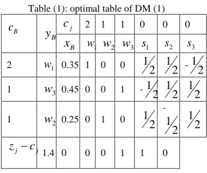
Table (1): optimal table of DM (1)

B

c

B

y

c

j 2 1 1 0 0 0 B

x

w

1

w

2

w

3

s

1

s

2

s

3

2

w

₁ 0.35 1 0 0

1

2

1

2

-

1

2

1

w

₃ 0.45 0 0 1 -

1

2

1

2

1

2

1

w

₂ 0.25 0 1 0

1

2

-1

2

1

2

j j

z



c

1.4 0 0 0 1 1 0

Hence the weight vector from DM(1) is

1

0.35,

2

0.45,

3

0.25

w



w



w



D.M (2):

Max z



2

w

₁



1

w

₂



1

w

₃

1 2

0.5;

1 3

0.7;

2 3

0.6;

1

,

2

,

3

0.

w



w



w



w



w



w



w w w



Solution:

1 2 3 1 2 3

2

1

0

Max z



w



w



w



s



s



s

1 2 1 2 3 1 3 1 2 3 2 3 1 2 3 1 2 3 1 2 3

0 0 0.5; 0 0 0.7

0 0 0.6; , , , , , 0

w w s s s w w s s s

w w s s s w w w s s s

         

     

Hence the weight vector from DM (2) is

1

0.3;

2

0.2;

3

0.4.

w



w



w



D.M (3):

Max z



2

w

₁



1

w

₂



1

w

₃

1 2

1 3

2 3 1 2 3

0.6;

0.9;

0.5;

,

0

w

w w w















Solution:

1 2 3 1 2 3

2

1

0

Max z



w



w



w



s



s



s

1 2 1 2 3 1 3 1 2 3

2 3 1 2 3 1 2 3 1 2 3

0

0.6;

0

0.9;

0

0.5; , , , , ,

0

w w s

s

w w

s s

s

w w

s

w w w s s s

    



Hence the weight vector from DM (3) is

1

0.5;

2

0.1;

3

0.4.

w



w



w



Construct a matrix with the vector obtained from the three decision makers as follows:

B

c

B

y

j

c

2 1 1 0 0 0

B

x

w

₁

w

₂

w

₃

s

₁

s

₂

s

₃

2

w

₁ 0.3 1 0 0

1

2

1

2

-

1

2

1

w

₃ 0.4 0 0 1 -

1

2

1

2

1

2

1

w

₂ 0.2 0 1 0

1

2

-

1

2

1

2

j j

[image:5.595.81.480.97.757.2] [image:5.595.65.274.550.724.2]

(6)

0.35 0.25 0.45

0.3

0.2

0.4

0.5

0.1

0.4

w









 











0.35

0.3

0.5

0.25 0.2

0.1

0.45 0.4

0.4

T

w









 











0.3594

0.2717

0.3686

V









 











Normalization of Solutions from Inverse Power Method

X

w

X





2.4 0.331950 2.4

3 0.336099 2.4 0.331950

8. NUMERICAL ILLUSTRATION

Let us suppose there is a risk investment company, which wants to invest a sum of money in the best option. There is a panel with five possible alternatives to invest the money. The risk investment company must take a decision according to the following four attributes: G1 is the risk analysis; G2 is the growth analysis; G3 is the social-political impact analysis; G4 is the environmental impact analysis.

The five possible alternatives



1, 2, 3, 4, 5



i

A i



are to be evaluated using intuitionistic fuzzy numbers by the three decision makers whose weighting vectorisobtained

by normalizing the solution of House Holder’s and inverse power methods are



0.36, 0.27, 0.37



T







0.33, 0.34, 0.33



T

w



under theabove four attributes whose weighting vector



0.2 0.1 0 ,

,

.3 0.4



T





and construct,

respectively, the decision matrices as listed in

the following matrices

 

2

5* 4



1, 2, 3



k ij

R



r

k



as follows:



 





 





 





 





 





 





 





 





 





 



1

0.3, 0.6

0.2, 0.7

0.7, 0.2

0.4, 0.5

0.5, 0.3

0.2, 0.3

0.3, 0.4

0.2, 0.6

0.7, 0.1

0.1, 0.3

0.5, 0.4 0.6, 0.3

0.7, 0.3 0.7, 0.2

0.6, 0.4 0.5, 0.4

0.8, 0.1 0.6, 0.3

0.6, 0.2 0.4, 0.3

R

















 





















 





 





 





 





 





 





 





 





 





 



2

0.4, 0.3

0.5, 0.2

0.2, 0.5

0.1, 0.6

0.6, 0.2

0.6, 0.1

0.3, 0.4

0.5, 0.3

0.4, 0.3

0.4, 0.2

0.5, 0.2

0.7, 0.1

0.5, 0.2

0.2, 0.3

0.1, 0.5

0.5, 0.1

0.3, 0.

2

0.6, 0.2

0.4, 0.2

R





































 





 





 





 





 





 





 





 





 





 



3

0.4, 0.5

0.5, 0.4

0.2, 0.7

0.1, 0.8

0.6, 0.4

0.6, 0.3

0.3, 0.6

0.5, 0.5

0.4, 0.5

0.4, 0.4

0.5, 0.4

0.7, 0.2

0.5, 0.4

0.2, 0.5

0.1, 0.7

0.5, 0.3

0.3, 0.4

0.6, 0.2

0.4, 0.4

R

















 



















Step-1:Utilize the IFWAA operator to derive the individual overall preference intuitionistic fuzzy values

r k

_i

 

of the alternative

A

_i is given by:

 1

1

(0.347222154, 0.549045978)

r



(1)

2

(0.604147627, 0.312913464)

r



(1)

3

(0.422920038, 0.327041507)

r



(1)

4

(0.456527711, 0.346410162)

r



(1)

5

(0.471481123, 0.198960391)

r



(2)

1

(0.244644753, 0.443076536)

r



B

c

B

y

c

j 2 1 1 0 0 0 B

x

w

₁

w

₂

w

₃

s

₁

s

₂

s

₃

2

w

₁ 0.5 1 0 0

1

2

1

2

-

1

2

1

w

₃ 0.4 0 0 1 -

1

2

1

2

1

2

1

w

₂ 0.2 0 1 0

1

2

-

1

2

1

2

j j

(7)

(2)

2

(0.499648495, 0.2)

r



(2)

3

(0.462173122, 0.225869387)

r



(2)

4

(0.342425064, 0.283679124)

r



(2)

5

(0.479785681, 0.174110113)

r



(3)

1

(0.244644753, 0.652777846)

r



(3)

2

(0.499648495, 0.419296271)

r



(3)

3

(0.462173122, 0.427693840)

r



(3)

4

(0.342425064, 0.465738581)

r



(3)

5

(0.479785681, 0.306734937)

r



Step 2. Utilize the IFHA operator to derive the collective overall preference intuitionistic fuzzy values

r

₁of the alternative

A

_iThen we have,

 1 1

(2) 1

(0.347222154, 0.549045978);

(0.244644753, 0.443076536)

r



(3)

1

(0.244644753, 0.652777846)

r







where





0.36, 0.27, 0.37

T



0.33, 0.34, 0.33



T

w



 

1

2

3

1

2

3

0.319047996;

0.319678982;

0.209543819

n

n n

b









 

1

2

3

1

2

3

0.523332094;

0.517187225;

0.622858796

n

n n

b







Utilizing IFHA operator we get,





,w 1

,

2

,

n

ITFHA

_

a a



a

   

1 1

1

(1

)

j

,

(

)

j

j j

n n

w w

a a

j j

 





 





 













Similarly we obtain:

1

(0.284926240, 0.552058815);

r



2

(0.540963409, 0.308604537);

r



3

(0.455857728, 0.326543318);

r



4

(0.387135173, 0.366150179);

r



5

(0.482762757, 0.225426377).

r



Step 3. Calculate the correlation coefficient between the collective overall preference values

i

r

_i, given as below:





















1 1

2 2

3 3

4 4

5 5

,

0.552058815;

,

0.308604537;

,

0.326543318;

,

0.366150179;

,

0.225426377.

ZL ZL ZL ZL ZL

C

r r

C

r r

C

r r

C

r r

C

r r



Step 4. The correlation coefficient of the IFSs, A and B is given by:





















1 1

2 2

3 3

4 4

5 5

0.859527561;

0.481661028;

0.542897490

0.624207596;

.

,

0.3710851 4

,

7

ZL ZL ZL ZL

ZL

r r





Step 5. Rank all the alternatives



1, 2, 3, 4, 5



i

A i



from the highest closeness (correlation coefficient) obtained from step 4, the result is as follows:

1 4 3 2 5

A



A



A



A



A

Hence, the best alternative is

A

₁.

9. CONCLUSION

In this work, we have discussed about the weight determining methods together with weighted averaging operator and the ordered weighted averaging operator. House-Holder and Inverse power methods were coupled with linear programming methods for determining the unknown decision maker weights. The proposed approach in this work not only can comfort the influence of unjust arguments on the decision results, but also avoid losing or distorting the original decision information in the process of aggregation.

REFERENCES

[1] Atanassov, K., (1999): Intuitionistic Fuzzy Sets. Theory and Applications, Physica-Verlag, Heidelberg, New York.

(8)

[3] Jain, M.K., Iyengar, S.R.K., & Jain, R.K., (2006): Numerical Methods for Scientific and Engineering Computation. Sixth Edition, New Age Publications.

[4] Robinson, J.P., & Amirtharaj, E.C.H., (2014): Efficient Multiple Attribute Group Decision Making Models with Correlation Coefficient of Vague sets. International Journal of Operations Research and Information Systems, 5 (3), pp. 27-51.

[5] Robinson, J.P., & Amirtharaj, E.C.H., (2015): MAGDM Problems with Correlation coefficient of Triangular Fuzzy IFS. International Journal of Fuzzy System Applications, 4 (1), pp. 1-32. [6] Wei, G., Wang H.J., & Lin,R. (2011):

Application of correlation coefficient to interval-valued intuitionistic fuzzy multiple attribute decision-making with incomplete weight information. Knowledge and Information Systems.26, pp. 337-349.

[7] Xu Z.S., (2007): Intuitionistic fuzzy aggregation operators. IEEE Transactions on Fuzzy Systems, 15 (6), pp. 1179–1187.

[8] Yager, R.R., (2004): Generalized OWA aggregation operators. Fuzzy Optimization and Decision Making, 3: pp. 93-107.

[9] Zadeh, L. A., (1965): Fuzzy sets. Information Control, 8, pp. 338-353.

[10]Zadeh, L.A., (1978): Fuzzy sets as a basis for a theory of possibility. Fuzzy Sets and Systems, 1, pp. 3-28.