Training Conditional Random Fields Using Incomplete Annotations

Training Conditional Random Fields Using Incomplete Annotations

Tokyo Research Laboratory, IBM Research, IBM Japan, Ltd Yamato, Kanagawa 242-8502, Japan {yutat,hkashima}@jp.ibm.com

Shinsuke Mori

Academic Center for Computing and Media Studies, Kyoto University Sakyo-ku, Kyoto 606-8501, Japan

[email protected]

Hiroki Oda Shinagawa, Tokyo, Japan [email protected]

Yuji Matsumoto

Graduate School of Information Science, Nara Institute of Science and Technology Takayama, Ikoma, Nara 630-0101, Japan

[email protected]

Abstract

We address corpus building situations, where complete annotations to the whole corpus is time consuming and unrealistic. Thus, annotation is done only on crucial part of sentences, or contains unresolved label ambiguities. We propose a parame-ter estimation method for Conditional Ran-dom Fields (CRFs), which enables us to use such incomplete annotations. We show promising results of our method as applied to two types of NLP tasks: a domain adap-tation task of a Japanese word segmenta-tion using partial annotasegmenta-tions, and a part-of-speech tagging task using ambiguous tags in the Penn treebank corpus.

1 Introduction

Annotated linguistic corpora are essential for building statistical NLP systems. Most of the corpora that are well-known in NLP communi-ties are completely-annotated in general. However it is quite common that the available annotations are partial or ambiguous in practical applications. For example, in domain adaptation situations, it is time-consuming to annotate all of the elements in a sentence. Rather, it is efficient to annotate certain parts of sentences which include domain-specific expressions. In Section 2.1, as an example of such efficient annotation, we will describe the effective-ness of partial annotations in the domain adapta-tion task for Japanese word segmentaadapta-tion (JWS). In addition, if the annotators are domain experts

c

2008. Licensed under the Creative Commons Attribution-Noncommercial-Share Alike 3.0 Unported li-cense (http://creativecommons.org/licenses/by-nc-sa/3.0/). Some rights reserved.

rather than linguists, they are unlikely to be confi-dent about the annotation policies and may prefer to be allowed to defer some linguistically complex decisions. For many NLP tasks, it is sometimes difficult to decide which label is appropriate in a particular context. In Section 2.2, we show that such ambiguous annotations exist even in a widely used corpus, the Penn treebank (PTB) corpus.

This motivated us to seek to incorporate such incomplete annotations into a state of the art ma-chine learning technique. One of the recent ad-vances in statistical NLP is Conditional Random Fields (CRFs) (Lafferty et al., 2001) that evaluate the global consistency of the complete structures for both parameter estimation and structure infer-ence, instead of optimizing the local configurations independently. This feature is suited to many NLP tasks that include correlations between elements in the output structure, such as the interrelation of part-of-speech (POS) tags in a sentence. However, conventional CRF algorithms require fully tated sentences. To incorporate incomplete anno-tations into CRFs, we extend the structured out-put problem in Section 3. We focus on partial an-notations or ambiguous anan-notations in this paper. We also propose a parameter estimation method for CRFs using incompletely annotated corpora in Section 4. The proposed method marginalizes out the unknown labels so as to optimize the likelihood of a set of possible label structures which are con-sistent with given incomplete annotations.

We conducted two types of experiments and ob-served promising results in both of them. One was a domain adaptation task for JWS to assess the proposed method for partially annotated data. The other was a POS tagging task using ambiguous an-notations that are contained in the PTB corpus. We summarize related work in Section 6, and conclude

ಾ ࠅ ் ߿ ߔ ࠅ ்

cut

incised wound

cut injury

abrasion or

file (or rasp)

infl. infl. infl. injury

pickpocket

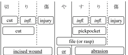
Figure 1: An example of word boundary ambigui-ties:infl.stands for an inflectional suffix of a verb.

in Section 7.

2 Incomplete Annotations 2.1 Partial Annotations

In this section, we describe an example of an effi-cient annotation which assigns partial word bound-aries for the JWS task.

It is not trivial to detect word boundaries for non-segmented languages such as Japanese or Chi-nese. For example, the correct segmentation of the Japanese phrase “੾Γই΍͢Γই” (incised

wound or abrasion) is shown by the lowest boxes segmented by the solid lines in Figure 1. How-ever, there are several overlapping segmentation candidates, which are shown by the other boxes, and possible segmentation by the dashed lines. Thus, the decisions on the word segmentation re-quire considering the context, so simple dictionary lookup approach is not appropriate. Therefore sta-tistical methods have been successfully used for JWS tasks. Previous work (Kudo et al., 2004) showed CRFs outperform generative Markov mod-els and discriminative history-based methods in JWS. In practice, a statistical word segment an-alyzer tends to perform worse for text from dif-ferent domains, so that additional annotations for each target domain are required. A major cause of errors is the occurrence of unknown words. For ex-ample, if “͢Γই” (abrasion) is an unknown word,

the system may accept the word sequence of “੾Γ ই΍͢Γই” as “੾Γই” (incised wound), “΍͢ Γ” (file), and “ই” (injury) by mistake.

On one hand, lists of new terms in the target domain are often available in the forms of techni-cal term dictionaries, product name lists, or other sources. To utilize those domain word lists, Mori (2006) proposed a KWIC (KeyWord In Context) style annotation user interface (UI) with which a user can delimit a word in a context with a single user action. In Figure 2, an annotator marks the oc-currences of “͢Γই”, a word in the domain word

ײછɺ֯ບͷ͜ ͢Γই ɺ֯ບ௵ᙾɺ

ൽෘʹ੾Γই΍ ͢Γই Λෛͬͨ৔߹

ట·ΈΕͷਂ͍ ͢Γই ΍ɺൽԼਂ͘

Figure 2: An example of KWIC style annotation: marked lines are identified as a correct segmenta-tion.

list, if they are used as a real word in their con-text. The “͢Γই” in the first row is a part of

an-other word “͜͢Γই” (scratch), and the annotator

marks the last two rows as correctly segmented ex-amples. This UI simplifies annotation operations for segmentation to yes/no decisions, and this sim-plification can also be effective for the reduction of the annotation effort for other NLP tasks. For example, the annotation operations for unlabeled dependency parsing can be simplified into a series of yes/no decisions as to whether or not given two words have syntactic dependency. Compared with sentence-wise annotation, the partial annotation is not only effective in terms of control operations, but also reduces annotation errors because it does not require annotating the word boundaries that an annotator is unsure of. This feature is crucial for annotations made by domain experts who are not linguists. 1 _{We believe partial annotation is}

effec-tive in creating corpora for many other structured annotations in the context of the domain adapta-tions.

2.2 Ambiguous Annotations

Ambiguous annotations in this paper refer to a set of candidate labels annotated for a part of a struc-tured instance. For example, the following sen-tence from the PTB corpus includes an ambiguous annotation for the POS tag of “pending”:

That/DT suit/NN is/VBZ pending/VBG|JJ ./. , where words are paired with their part-of-speech tag by a forward slash (“/”).2_Uncertainty

concern-ing the proper POS tag of “pendconcern-ing” is represented by the disjunctive POS tag (“VBG and JJ”) as in-dicated by a vertical bar.

The existence of the ambiguous annotations is due to the task definition itself, the procedure man-1_{The boundary policies of some words are different even} among linguists. In addition, the boundary agreement is even lower in Chinese (Luo, 2003).

frequency word POS tags 15 data NN|NNS 10 more JJR|RBR 7 pending JJ|VBG 4 than IN|RB

Table 1: Words in the PTB with ambiguous POSs.

ual for the annotators, or the inadequate knowl-edge of the annotators. Ideally, the annotations should be disambiguated by a skilled annotator for the training data. However, even the PTB cor-pus, whose annotation procedure is relatively well-defined, includes more than 100 sentences contain-ing POS ambiguities such as those listed in Ta-ble 1. Although the number of ambiguous an-notations is not considerably large in PTB cor-pus, corpora could include more ambiguous anno-tations when we try to build wider coverage cor-pora. Also, ambiguous annotations are more com-mon in the tasks that deal with semantics, such as information extraction tasks so that learning algo-rithms must deal with ambiguous annotations.

3 Problem Definition

In this section, we give a formal definition of the supervised structured output problem that uses par-tial annotations or ambiguous annotations in the training phase. Note that we assume the input and output structures are sequences for the purpose of explanation, though the following discussion is ap-plicable to other structures, such as trees.

Let x=(x1, x2,· · · , xT) be a sequence of

ob-served variables xt ∈ X andy=(y1, y2,· · · , yT)

be a sequence of label variablesyt∈Y. Then the

supervised structured output problem can be de-fined as learning a mapX → Y. In the Japanese word segmentation task, x can represent a given sequence of character boundaries and y is a se-quence of the corresponding labels, which spec-ify whether the current position is a word bound-ary.3 _{In the POS tagging task,xrepresents a word}

sequence and y is a corresponding POS tag se-quence. An incomplete annotation, then, is defined as a sequence of subset of the label set instead of a sequence of labels. LetL=(L1, L2,· · · , LT)be a

sequence of label subsets for an observed sequence 3_{Peng et al. (2004) defined the word segmentation} prob-lem as labeling each character as whether or not the previous character boundary of the current character is a word bound-ary. However, we employ our problem formulation since it is redundant to assign the first character of a sentence as the word boundary in their formulation.

x, whereLt ∈ 2Y − {∅}. The partial annotation

at positionsis whereLsis a singleton and the rest

Lt=sisY. For example, if a sentence with 6

char-acter boundaries (7 charchar-acters) is partially anno-tated using the KWIC UI described in Section 2.1, a word annotation where its boundary begins with

t= 2and ends witht= 5will be represented as:

L= ({,×},{} ,{×},{×},{}

partial annotation

,{,×}),

where and × denote the word boundary la-bel and the non-word boundary lala-bel, respectively. The ambiguous annotation is represented as a set which contains candidate labels. The example sen-tence including the ambiguous POS tag in Sec-tion 2.2 can be represented as:

L= ({DT},{NN},{VBZ}, { VBG,JJ}

ambiguous annotation

,{.}).

Note that, if all the elements of a given sequence are annotated, it is the special case such that the size of all elements is one, i.e. |Lt| = 1 for all

t = 1,· · · , T. The goal in this paper is training a statistical model from partially or ambiguously annotated data,D={(x(n)_,L(n)_)}N

n=1.

4 Marginalized Likelihood for CRFs

In this section, we propose a parameter estimation procedure for the CRFs (Lafferty et al., 2001) in-corporating partial or ambiguous annotations. Let

Φ(x,y) :X×Y → d_{denote a map from a pair}

of an observed sequencexand a label sequencey to an arbitrary feature vector ofddimensions, and θ ∈ d _{denotes the vector of the model}

parame-ters. CRFs model the conditional probability of a label sequenceygiven an observed sequencexas:

P„(y|x) = e_Z„·Φ(x,y)

„,x,Y ɼ (1)

where ·denotes the inner product of the vectors, and the denominator is the normalization term that guarantees the model to be a probability:

Z„,x,S =

y∈S

e„·Φ(x,y)_.

Then once θ has been estimated, the la-bel sequence can be predicted by yˆ = argmaxy∈Y P„(y|x). Since the original CRF

learning algorithm requires a completely labeled sequence y, the incompletely annotated data

LetYLdenote all of the possible label sequence

consistent with L. We propose to use the condi-tional probability of the subsetYLgivenx:

P„(YL|x) =

y∈Y_L

P„(y|x), (2)

which marginalizes the unknown ys out. Then the maximum likelihood estimator for this model can be obtained by maximizing the log likelihood function:

LL(θ) =N n=1

lnP„(YL(n)|x(n)) (3)

= N

n=1

lnZ„,x(n)_,Y

L(n) −lnZ„,x(n),Y

.

This modeling naturally embraces label ambigui-ties in the incomplete annotation.4

Unfortunately, equation (3) is not a concave function5 _{so that there are local maxima in the}

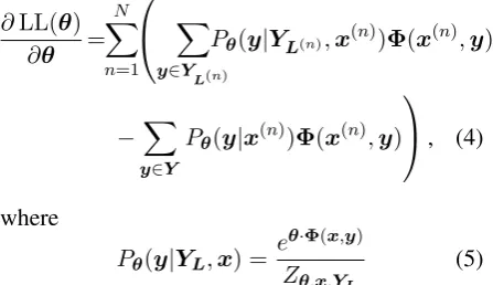
objective function. Although this non-concavity prevents efficient global maximization of equation (3), it still allows us to incorporate incomplete an-notations using gradient ascent iterations (Sha and Pereira, 2003). Gradient ascent methods require the partial derivative of equation (3):

∂LL(θ)

∂θ =

N

n=1

⎛

⎝

y∈Y_L(n)

P„(y|YL(n),x(n))Φ(x(n),y)

−

y∈Y

P„(y|x(n)_)Φ(x(n)_,y)

⎞ ⎠_{, (4)}

where

P„(y|YL,x) = e

„·Φ(x,y)

Z„,x,Y_L (5)

is a conditional probability that is normalized over YL.

Equations (3) and (4) include the summations of all of the label sequences inY orYL. It is not

practical to enumerate and evaluate all of the label configurations explicitly, since the number of all of the possible label sequences is exponential on the number of positionstwith|Lt|>1. However,

un-der the Markov assumption, a modification of the 4_{It is common to introduce a prior distribution over the} pa-rameters to avoid over-fitting in CRF learning. In the experi-ments in Section 5, we used a Gaussian prior with the mean0 and the varianceσ2_{so that−}||„||2

2σ2 is added to equation (3).

5_{Since its second order derivative can be positive.}

domain #sentences #words (A) conversation 11,700 145,925 (B) conversation 1,300 16,348 (C) medical manual 1,000 29,216

Table 2: Data statistics.

Types Template

Characters c−1, c+1,

Character types c−2c−1, c−1c+1, c+1c+2,

Term in dic. c−2c−1c+1, c−1c+1c+2

Term in dic. starts at _c −1, c+1

Term in dic. ends at

Table 3: Feature templates: Each subscript stands for the relative distance from a character boundary.

Forward-Backward algorithm guarantees polyno-mial time computation for the equations (3) and (4). We explain this algorithm in Appendix A.

5 Experiments

We conducted two types of experiments, assessing the proposed method in 1) a Japanese word seg-mentation task using partial annotations and 2) a POS tagging task using ambiguous annotations.

5.1 Japanese Word Segmentation Task In this section, we show the results of domain adaptation experiments for the JWS task to assess the proposed method. We assume that only par-tial annotations are available for the target domain. In this experiment, the corpus for the source do-main is composed of example sentences in a dic-tionary of daily conversation (Keene et al., 1992). The text data for the target domain is composed of sentences in a medical reference manual (Beers, 2004) . The sentences of all of the source domain corpora (A), (B) and a part of the target domain text (C) were manually segmented into words (see Table 2).

The performance measure in the experiments is the standard F measure score,F = 2RP/(R+P)

where

R= _{# of words in test data}# of correct words ×100

P = _{# of words in system output}# of correct words ×100.

91 91.5 92 92.5 93 93.5 94 94.5 95

0 100 200 300 400 500 600 700 800 900 1000 Number of word annotations

F

Proposed method Argmax as training data Point-wise classifier

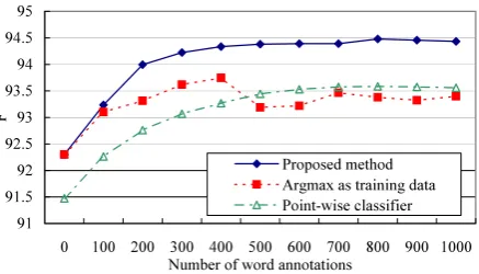
Figure 3: Average performances varying the num-ber of word annotations over 2 trials.

data for annotation and training (C1) versus the data for testing (C2).

We implemented first order Markov CRFs. As the features for the observed variables, we use the characters and character type n-gram (n=1,2,3) around the current character boundary. The character types are categorized into Hiragana, Katakana,Kanji, English alphabet, Arabic numer-als, and symbols. We also used lexical features consulting a dictionary: one is to check if any of the above defined charactern-grams appear in a dictionary (Peng et al., 2004), and the other is to check if there are any words in the dictionary that start or end at the current character boundary. We used theunidic6 _{(281K distinct words) as the}

general purpose dictionary, and theJapanese Stan-dard Disease Code Master (JSDCM)7 _(23K

dis-tinct words) as the medical domain dictionary. The templates for the features we used are summarized in Table 3. To reduce the number of parameters, we selected only frequent features in the source do-main data (A) or in about50Kof the unsegmented sentences of the target domain.8 _{The total number}

of distinct features was about300K.

A CRF that was trained using only the source domain corpus (A), CRFS_{, achievedF=96.84 in}

the source domain validation data (B). However, it showed the need for the domain adaptation that this CRFS _{suffered severe performance}

degrada-tion (F=92.3) on the target domain data. This experiment was designed for the case in which a user selects the occurrences of words in the word list using the KWIC interface described in Sec-tion 2.1. We employed JSDCM as a word list in which 224 distinct terms appeared on average over 2 test sets (C1). The number of word

an-6_{Ver. 1.3.5; http://www.tokuteicorpus.jp/dist/} 7_{Ver. 2.63; http://www2.medis.or.jp/stdcd/byomei/} 8_{The data (B) and (C), which were used for validation and} test, were excluded from this feature selection process.

notations varied from 100to 1000 in this exper-iment. We prioritized the occurrences of each word in the list using a selective sampling tech-nique. We used label entropy (Anderson et al., 2006), H(ys

t) = ys

t∈YtsP„˜(y

s

t|x) lnP„˜(yts|x)

, as importance metric of each word occurrence, whereθ˜is the model parameter of CRFS_{, andy}s

t = (yt, yt+1,· · ·, ys) ∈ Ytsis a subsequence starting

att and ending at sin y. Intuitively, this metric represents the prediction confidence of CRFS_.9 _As

training data, we mixed the complete annotations (A) and these partial annotations on data (C1) be-cause that performance was better than using only the partial annotations.

We usedconjugate gradientmethod to find the local maximum value with the initial value being set to be the parameter vector of CRFS_{. Since the}

amount of annotated data for the target domain was limited, the hyper-parameterσ was selected using the corpus (B).

For the comparison with the proposed method, the CRFs were trained using the most probable label sequences consistent with L (denoted as argmax). The most probable label sequences were predicted by the CRFS_{. Also, we used apoint-wise}

classifier, which independently learns/classifies each character boundary and just ignores the unan-notated positions in the learning phase. As the point-wise classifier, we implemented a maximum entropy classifier which uses the same features and optimizer as CRFs.

Figure 3 shows the performance comparisons varying the number of word annotations. The combination of both the proposed method and the selective sampling method showed that a small number of word annotations effectively improved the word segmentation performance. In addi-tion, the proposed method significantly outper-formedargmaxandpoint-wise classifierbased on the Wilcoxon signed rank test at the significance level of 5%. This result suggests that the pro-posed method maintains CRFs’ advantage over the point-wise classifierand properly incorporates par-tial annotations.

5.2 Part-of-speech Tagging Task

In this section, we show the results of the POS tag-ging experiments to assess the proposed method using ambiguous annotations.

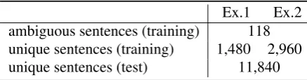
Ex.1 Ex.2 ambiguous sentences (training) 118 unique sentences (training) 1,480 2,960 unique sentences (test) 11,840 Table 4: Training and test data for POS tagging.

As mentioned in Section 2.2, there are words which have two or more candidate POS tags in the PTB corpus (Marcus et al., 1993). In this experi-ment, we used 118 sentences in which some words (82 distinct words) are annotated with ambiguous POS tags, and these sentences are called thePOS ambiguous sentences. On the other hand, we call sentences in which the POS tags of these terms are uniquely annotated as thePOS unique sentences.

The goal of this experiment is to effectively im-prove the tagging performance using both these POS ambiguous sentences and the POS unique sentences as the training data. We assume that the amount of training data is not sufficient to ignore the POS ambiguous sentences, or that the POS am-biguous sentences make up a substantial portion of the total training data. Therefore we used a small part (1/10or1/5) of the POS unique sentences for training the CRFs and evaluated their performance using other (4/5) POS unique sentences. We con-ducted two experiments in which different num-bers of unique sentences were used in the training phases, and these settings are summarized in Ta-ble 4.

The feature sets for each word are the case-insensitive spelling, the orthographic features of the current word, and the sentence’s last word. The orthographic features are whether a spelling begins with a number or an upper case letter; whether it begins with an upper case letter and contains a period (“.”); whether it is all upper case letters or all lower case letters; whether it contains a punc-tuation mark or a hyphen; and the last one, two, and three letters of the word. Also, the sentence’s last word corresponds to a punctuation mark (e.g. “.”, “?”, “!”). We employed only features that ap-peared more than once. The total number of re-sulting distinct features was about14K. Although some symbols are treated as distinct tags in the PTB tag definitions, we aggregated these symbols into a symbol tag (SYM) since it is easy to restore original symbol tags from the SYM tag. Then, the number of the resulting tags was 36.

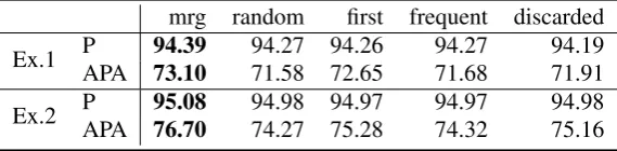
For the comparison with the proposed method (mrg), we used three heuristic rules that disam-biguated the annotated candidate POS tags in the

POS ambiguous sentences. These rules selected a POS tag 1) at random, 2) as the first one in the description order10_{, 3) as the most frequent tag}

in the corpus. In addition, we evaluated the case when the POS ambiguous sentences are 4) dis-cardedfrom the training data.

For evaluation, we employed the Precision (P) and Average Precision for Ambiguous words (APA):

P=# of correctly tagged word_{# of all word occurrences} ×100ɼ

APA=_|A1_| w∈A

# of the correctly taggedw

# of all occurrences ofw ×100ɼ

whereAis a word set and is composed of the word for which at least one of its occurrences is ambigu-ously annotated. Here, we employed APA to eval-uate each ambiguous words equally, and|A|was 82 in this experiment. Again, we used the conju-gate gradient method to find the local maximum value with the initial value being set to be the pa-rameters obtained in the CRF learning for the dis-cardedsetting.

Table 5 shows the average performance of POS tagging over 5 different POS unique data. Since the POS ambiguous sentences are only a fraction of all of the training data, the overall performance (P) was slightly improved by the proposed method. However, according to the performance for am-biguously annotated words (APA), the proposed method outperformed other heuristics for POS dis-ambiguation. The P and APA scores between the proposed method and the comparable methods are significantly different based on the Wilcoxon signed rank testat the 5% significance level. Al-though the performance improvement in this POS tagging task was moderate, we believe the pro-posed method will be more effective to the NLP tasks whose corpus has a considerable number of ambiguous annotations.

6 Related Work

Pereira and Schabes (1992) proposed a grammar acquisition method for partially bracketed corpus. Their work can be considered a generative model for the tree structure output problem using partial annotations. Our discriminative model can be ex-tended to such parsing tasks.

mrg random first frequent discarded Ex.1 P_APA 94.39_73.10 94.27 94.26_{71.58 72.65} 94.27_71.68 94.19_71.91

Ex.2 P_APA 95.08_76.70 94.98 94.97_{74.27 75.28} 94.97_74.32 94.98_75.16 Table 5: The average POS tagging performance over 5 trials. Our model is interpreted as one of the CRFs

with hidden variables (Quattoni et al., 2004). There are previous work which handles hidden variables in discriminative parsers (Clark and Cur-ran, 2006; Petrov and Klein, 2008). In their meth-ods, the objective functions are also formulated as same as equation (3).

For interactive annotation, Culotta et al. (2006) proposed corrective feedback that effectively re-duces user operations utilizing partial annotations. Although they assume that the users correct en-tire label structures so that the CRFs are trained as usual, our proposed method extends their system when the users cannot annotate all of the labels in a sentence.

7 Conclusions and Future Work

We are proposing a parameter estimation method for CRFs incorporating partial or ambiguous an-notations of structured data. The empirical results suggest that the proposed method reduces the do-main adaptation costs, and improves the prediction performance for the linguistic phenomena that are sometimes difficult for people to label.

The proposed method is applicable to other structured output tasks in NLP, such as syntactic parsing, information extraction, and so on. How-ever, there are some NLP tasks, such as the word alignment task (Taskar et al., 2005), in which it is not possible to efficiently calculate the sum score of all of the possible label configurations. Re-cently, Verbeek and Triggs (2008) independently proposed a parameter estimation method for CRFs using partially labeled images. Although the ob-jective function in their formulation is equivalent to equation (3), they used Loopy Belief Propaga-tion to approximate the sum score for their ap-plication (scene segmentation). Their results im-ply these approximation methods can be used for such applications that cannot use dynamic pro-gramming techniques.

Acknowledgments

We would like to thank the anonymous reviewers for their comments. We also thank Noah Smith,

Ryu Iida, Masayuki Asahara, and the members of the T-PRIMAL group for many helpful discus-sions.

References

Anderson, Brigham, Sajid Siddiqi, and Andrew Moore. 2006. Sequence selection for active learning. Tech-nical Report CMU-IR-TR-06-16, Carnegie Mellon University.

Beers, Mark H. 2004. The Merck Manual of Medical

Information (in Japanese). Nikkei Business

Publi-cations, Inc, Home edition.

Clark, Stephen and James R. Curran. 2006. Par-tial training for a lexicalized-grammar parser. In

Proceedings of the Annual Meeting of the North American Association for Computational Linguis-tics, pages 144–151.

Culotta, Aron, Trausti Kristjansson, Andrew McCal-lum, and Paul Viola. 2006. Corrective feedback and persistent learning for information extraction.

Artifi-cial Intelligence Journal, 170:1101–1122.

Keene, Donald, Hiroyoshi Hatori, Haruko Yamada, and Shouko Irabu, editors. 1992. Japanese-English

Sen-tence Equivalents (in Japanese). Asahi Press,

Elec-tronic book edition.

Kudo, Taku, Kaoru Yamamoto, and Yuji Matsumoto. 2004. Applying conditional random fields to Japanese morphological analysis. InProceedings of

Empirical Methods in Natural Language Processing.

Lafferty, John, Andrew McCallum, and Fernando Pereira. 2001. Conditional random fields: Proba-bilistic models for segmenting and labeling sequence data. InProceedings of the 18th International

Con-ference on Machine Learning.

Luo, Xiaoquan. 2003. A maximum entropy chinese character-based parser. InProceedings of the Con-ference on Empirical Methods in Natural Language

Processing, pages 192–199.

Marcus, Mitchell P., Mary Ann Marcinkiewicz, and Beatrice Santorini. 1993. Building a large annotated corpus of English: The Penn treebank.

Computa-tional Linguistics, 19(2).

Mori, Shinsuke. 2006. Language model adaptation with a word list and a raw corpus. InProceedings of the 9th International Conference on Spoken

Peng, Fuchun, Fangfang Feng, and Andrew McCallum. 2004. Chinese segmentation and new word detection using conditional random fields. InProceedings of the International Conference on Computational

Lin-guistics.

Pereira, Fernando C. N. and Yves Schabes. 1992. Inside-outside reestimation from partially bracketed corpora. InProceedings of Annual Meeting

Associ-ation of ComputAssoci-ational Linguistics, pages 128–135.

Petrov, Slav and Dan Klein. 2008. Discriminative log-linear grammars with latent variables. In

Ad-vances in Neural Information Processing Systems,

pages 1153–1160, Cambridge, MA. MIT Press. Quattoni, Ariadna, Michael Collins, and Trevor Darrell.

2004. Conditional random fields for object recogni-tion. InAdvances in Neural Information Processing

Systems.

Sha, Fei and Fernando Pereira. 2003. Shallow pars-ing with conditional random fields. In Proceedings

of Human Language Technology-NAACL,

Edmon-ton, Canada.

Taskar, Ben, Simon Lacoste-Julien, and Dan Klein. 2005. A discriminative matching approach to word alignment. InProceedings of the Conference on

Em-pirical Methods in Natural Language Processing.

Verbeek, Jakob and Bill Triggs. 2008. Scene segmen-tation with CRFs learned from partially labeled im-ages. InAdvances in Neural Information Processing

Systems, pages 1553–1560, Cambridge, MA. MIT

Press.

Appendix A Computation of Objective and Derivative functions

Here we explain the effective computation proce-dure for equation (3) and (4) using dynamic pro-gramming techniques.

Under the first-order Markov assumption11_{, two}

types of features are usually used: one is pairs of an observed variable and a label variable (denoted as f(xt, yt) : X ×Y), the other is pairs of two

label variables (denoted as g(yt−1, yt) : Y ×Y)

at time t. Then the feature vector can be de-composed as Φ(x,y) = T_t=1+1φ(xt, yt−1, yt)

where φ(xt, yt−1, yt) = f(xt, yt) +g(yt−1, yt).

In addition, let S and E be special label vari-ables to encode the beginning and ending of a se-quence, respectively. We defineφ(xt, yt−1, yt)to

beφ(xt, S, yt)at the headt= 1andg(yt−1, E)at

the tail wheret=T + 1. The technique of the ef-fective calculation of the normalization value is the 11_{Note that, although the rest of the explanation based on} the first-order Markov models for purposes of illustration, the following arguments are easily extended to the higher order Markov CRFs and semi-Markov CRFs.

precomputation of theα„,x,L[t, j],andβ„,x,L[t, j]

matrices with givenθ,x, andL. The matricesα

andβ are defined as follows, and should be cal-culated in the order of t = 1,· · · , T, and t =

T+ 1,· · · ,1, respectively

α„,x,L[t, j]

=

⎧ ⎪ ⎪ ⎪ ⎨ ⎪ ⎪ ⎪ ⎩

0 ifj /∈Lt

θ·φ(xt, S, j) else ift= 1

ln

i∈Lt−1

eα[t−1,i]+„·ffi(xt,i,j) _else

β„,x,L[t, j]

=

⎧ ⎪ ⎪ ⎪ ⎨ ⎪ ⎪ ⎪ ⎩

0 ifj /∈Lt

θ·g(j, E) else ift=T+ 1

ln

k∈Lt+1

e„·ffi(xt,j,k)+β[t+1,k] _else

Note thatL = (Y,· · · , Y)is used to calculate all the entries inY. In the rest of this section, we omit the subscripts θ,x, andL of α, β, Z unless mis-understandings could occur. The time complexity of theα[t, j]orβ[t, j]computation isO(T|Y|2_).

Finally, equations (3) and (4) are efficiently cal-culated usingα, β. The logarithm ofZin equation (3) is calculated as:

lnZ„,Y_L = ln

j∈LT

eα„,L[T,j]+„·g(j,E).

Similarly, the first and second terms of equation (4) can be computed as:

y∈Y_L

P„,L(y|x)Φ(x,y) =

i∈LT

εL(T, i, E)g(i, E)

+ T

t=1

j∈Lt ⎛

⎝_{γL(t, j)f(xt, j) +}

i∈Lt−1

εL(t, i, j)g(i, j)

⎞ ⎠

whereθ,xare omitted in this equation, andγ„,x,L

andε„,x,Lare the marginal probabilities:

γ„,x,L(t, j) =P„,L(yt=j|x)

=eα[t,j]+β[t,j]−lnZ_{YL, and}

ε„,x,L(t, i, j) =P„,L(yt−1=i, yt=j|x) =eα[t−1,i]+„·ffi(xt,i,j)+β[t,j]−lnZ_YL.