Automatic Identification of Non-Compositional Multi-Word Expressions
using Latent Semantic Analysis
Graham Katz
Institute of Cognitive Science University of Osnabr¨uck
Eugenie Giesbrecht
Institute of Cognitive Science University of Osnabr¨uck
Abstract
Making use of latent semantic analy-sis, we explore the hypothesis that lo-cal linguistic context can serve to iden-tify multi-word expressions that have non-compositional meanings. We propose that vector-similarity between distribution vec-tors associated with an MWE as a whole and those associated with its constitutent parts can serve as a good measure of the degree to which the MWE is composi-tional. We present experiments that show that low (cosine) similarity does, in fact, correlate with non-compositionality.
1 Introduction
Identifying non-compositional (or idiomatic) multi-word expressions (MWEs) is an important subtask for any computational system (Sag et al., 2002), and significant attention has been paid to practical methods for solving this problem in recent years (Lin, 1999; Baldwin et al., 2003; Villada Moir´on and Tiedemann, 2006). While corpus-based techniques for identifying collo-cational multi-word expressions by exploiting statistical properties of the co-occurrence of the component words have become increasingly sophisticated (Evert and Krenn, 2001; Evert, 2004), it is well known that mere co-occurrence does not well distinguish compositional from non-compositional expressions (Manning and Sch¨utze, 1999, Ch. 5).
While expressions which may potentially have idiomatic meanings can be identified using various lexical association measures (Evert and Krenn, 2001; Evert and Kermes, 2003), other techniques must be used to determining whether or not a par-ticular MWE does, in fact, have an idiomatic use.
In this paper we explore the hypothesis that the local linguistic context can provide adequate cues for making this determination and propose one method for doing this.
We characterize our task on analogy with word-sense disambiguation (Sch¨utze, 1998; Ide and V´eronis, 1998). As noted by Sch¨utze, WSD involves two related tasks: the general task of sense discrimination—determining what senses a given word has—and the more specific task of sense selection—determining for a particular use of the word in context which sense was in-tended. For us the discrimination task involves determining for a given expression whether it has a non-compositional interpretation in addition to its compositional interpretation, and the selec-tion task involves determining in a given context, whether a given expression is being used compo-sitionally or non-compostionally. The German ex-pression ins Wasser fallen, for example, has a non-compositional interpretation on which it means ‘to fail to happen’ (as in (1)) and a compositional in-terpretation on which it means ‘to fall into water (as in (2)).1
(1) Das Kind war beim Baden von einer
Luftma-tratze ins Wasser gefallen.
‘The child had fallen into the water from an a air matress while swimming’
(2) Die Er¨ofnung des Skateparks ist ins Wasser
gefallen.
‘The opening of the skatepark was cancelled’
The discrimination task, then, is to identify ins
Wasser fallen as an MWE that has an idiomatic
meaning and the selection task is to determine that
1Examples taken from a newspaper corpus of the German
S¨uddeutsche Zeitung (1994-2000)
in (1) it is the compositional meaning that is in-tended, while in (2) it is the non-compositional meaning.
Following Sch¨utze (1998) and Landauer & Du-mais (1997) our general assumption is that the meaning of an expression can be modelled in terms of the words that it co-occurs with: its co-occurrence signature. To determine whether a phrase has a non-compositional meaning we compute whether the co-occurrence signature of the phrase is systematically related to the co-occurrence signatures of its parts. Our hypoth-esis is that a systematic relationship is indica-tive of compositional interpretation and lack of a systematic relationship is symptomatic of non-compositionality. In other words, we expect com-positional MWEs to appear in contexts more sim-ilar to those in which their component words ap-pear than do non-compositional MWEs.
In this paper we describe two experiments that test this hypothesis. In the first experiment we seek to confirm that the local context of a known idiom can reliably distinguish idiomatic uses from non-idiomatic uses. In the second experiment we attempt to determine whether the difference be-tween the contexts in which an MWE appears and the contexts in which its component words appear can indeed serve to tell us whether the MWE has an idiomatic use.
In our experiments we make use of lexical se-mantic analysis (LSA) as a model of context-similarity (Deerwester et al., 1990). Since this technique is often used to model meaning, we will speak in terms of “meaning” similiarity. It should be clear, however, that we are only using the LSA vectors—derived from context of occurrence in a corpus—to model meaning and meaning composi-tion in a very rough way. Our hope is simply that this rough model is sufficient to the task of identi-fying non-compositional MWEs.
2 Previous work
Recent work which attempts to discriminate between compositional and non-compositional MWEs include Lin (1999), who used mutual-information measures identify such phrases, Bald-win et al. (2003), who compare the distribution of the head of the MWE with the distribution of the entire MWE, and Vallada Moir´on & Tiede-mann (2006), who use a word-alignment strat-egy to identify non-compositional MWEs making
use of parallel texts. Schone & Jurafsky (2001) applied LSA to MWE identification, althought they did not focus on distinguishing compositional from non-compositional MWEs.
Lin’s goal, like ours, was to discriminate non-compositional MWEs from non-compositional MWEs. His method was to compare the mutual informa-tion measure of the constituents parts of an MWE with the mutual information of similar expressions obtained by substituting one of the constituents with a related word obtained by thesaurus lookup. The hope was that a significant difference between these measures, as in the case of red tape (mutual information: 5.87) compared to yellow tape (3.75) or orange tape (2.64), would be characteristic of non-compositional MWEs. Although intuitively appealing, Lin’s algorithm only achieves precision and recall of 15.7% and 13.7%, respectively (as compared to a gold standard generate from an id-iom dictionary—but see below for discussion).
Schone & Jurafsky (2001) evaluated a num-ber of co-occurrence-based metrics for identify-ing MWEs, showidentify-ing that, as suggested by Lin’s results, there was need for improvement in this area. Since LSA has been used in a number of meaning-related language tasks to good ef-fect (Landauer and Dumais, 1997; Landauer and Psotka, 2000; Cederberg and Widdows, 2003), they had hoped to improve their results by identify non-compositional expressions using a method similar to that which we are exploring here. Al-though they do not demonstrate that this method actually identifies non-compositional expressions, they do show that the LSA similarity technique only improves MWE identification minimally.
to be more an indication of the inappropriateness of the evaluation used than of the faultiness of the general approach.
Lin, Baldwin et al., and Schone & Jurafsky, all use as their gold standard either idiom dictionaries or WordNet (Fellbaum, 1998). While Schone & Jurafsky show that WordNet is as good a standard as any of a number of machine readable dictionar-ies, none of these authors shows that the MWEs that appear in WordNet (or in the MRDs) are gen-erally non-compositional, in the relevant sense. As noted by Sag et al. (2002) many MWEs are sim-ply “institutionalized phrases” whose meanings are perfectly compositional, but whose frequency of use (or other non-linguistic factors) make them highly salient. It is certainly clear that many MWEs that appear in WordNet—examples being
law student, medical student, college man—are
perfectly compositional semantically.
Zhai (1997), in an early attempt to apply statistical methods to the extraction of non-compositional MWEs, made use of what we take to be a more appropriate evaluation metric. In his comparison among a number of different heuris-tics for identifying non-compositional noun-noun compounds, Zhai did his evaluation by applying each heuristic to a corpus of items hand-classified as to their compositionality. Although Zhai’s clas-sification appears to be problematic, we take this to be the appropirate paradigm for evaluation in this domain, and we adopt it here.
3 Proceedure
In our work we made use of the Word Space model of (semantic) similiarty (Sch¨utze, 1998) and extended it slightly to MWEs. In this frame-work, “meaning” is modeled as an n-dimensional vector, derived via singular value decomposition (Deerwester et al., 1990) from word co-occurrence counts for the expression in question, a technique frequently referred to as Latent Semantic Analysis (LSA). This kind of dimensionality reduction has been shown to improve performance in a number of text-based domains (Berry et al., 1999).
For our experiments we used a local German newspaper corpus.2 We built our LSA model with the Infomap Software package.3, using the 1000 most frequent words not on the 102-word
2
S¨uddeutsche Zeitung (SZ) corpus for 2003 with about 42 million words.
[image:3.595.336.502.78.187.2]3Available frominfomap.stanford.edu.
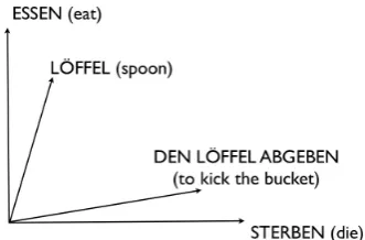
Figure 1: Two dimensional Word Space
hand-generated stop list as the content-bearing di-mension words (the columns of the matrix). The 20,000 most frequent content words were assigned row values by counting occurrences within a 30-word window. SVD was used to reduce the di-mensionality from 1000 to 100, resulting in 100 dimensional “meaning”-vectors for each word. In our experiments, MWEs were assigned meaning-vectors as a whole, using the same proceedure. For meaning similarity we adopt the standard mea-sure of cosine of the angle between two vectors (the normalized correlation coefficient) as a met-ric (Sch¨utze, 1998; Baeza-Yates and Ribeiro-Neto, 1999). On this metric, two expressions are taken to be unrelated if their meaning vectors are orthog-onal (the cosine is 0) and synonymous if their vec-tors are parallel (the cosine is 1).
Figure 1 illustrates such a vector space in two dimensions. Note that the meaning vector for
L¨offel ‘spoon’ is quite similar to that for es-sen ‘to eat’ but distant from sterben ‘to die’,
while the meaning vector for the MWE den L¨offel
abgeben is close to that for sterben. Indeed den L¨offel abgeben, like to kick the bucket, is a
non-compositional idiom meaning ‘to die’.
While den L¨offel abgeben is used almost ex-clusively in its idiomatic sense (all four occur-rences in our corpus), many MWEs are used reg-ularly in both their idiomatic and in their literal senses. About two thirds of the uses of the MWE
ins Wasser fallen in our corpus are idiomatic uses,
3.1 Experiment I
For this experiment we manually annotated the 67 occurrences of ins Wasser fallen in our cor-pus as to whether the expression was used com-positionally (literally) or non-comcom-positionally (id-iomatically).4 Marking this distinction we gen-erate an LSA meaning vectors for the composi-tional uses and an LSA meaning vector for the non-compositional uses of ins Wasser fallen. The vectors turned out, as expected, to be almost or-thogonal, with a cosine of the angle between them of 0.02. This result confirms that the linguis-tic contexts in which the literal and the idiomalinguis-tic use of ins Wasser fallen appear are very differ-ent, indicating—not surprisingly—that the seman-tic difference between the literal meaning and the idiomatic meaning is reflected in the way these these phrases are used.
Our next task was to investigate whether this difference could be used in particular cases to de-termine what the intended use of an MWE in a particular context was. To evaluate this, we did a 10-fold cross-validation study, calculating the lit-eral and idiomatic vectors for ins Wasser fallen on the basis of the training data and doing a simple nearest neighbor classification of each memember of the test set on the basis of the meaning vectors computed from its local context (the 30 word win-dow). Our result of an average accurace of 72% for our LSA-based classifier far exceeds the sim-ple maximum-likelihood baseline of 58%.
In the final part of this experiment we compared the meaning vector that was computed by sum-ming over all uses of ins Wasser fallen with the literal and idiomatic vectors from above. Since id-iomatic uses of ins Wasser fallen prevail in the cor-pus (2/3 vs. 1/3), it is not surprisingly that the sim-ilarity to the literal vector (0.0946) is much than similarity to the idiomatic vector (0.3712).
To summarize Experiment I, which is a vari-ant of a supervised phrase sense disambiguation task, demonstrates that we can use LSA to distin-guish between literal and the idiomatic usage of an MWE by using local linguistic context.
4This was a straightforward task; two annotators
anno-tated independently, with very high agreement—kappa score of over 0.95 (Carletta, 1996). Occurrences on which the an-notators disagreed were thrown out. Of the 64 occurrences we used, 37 were idiomatic and 27 were literal.
3.2 Experiment II
In our second experiment we sought to make use of the fact that there are typically clear distributional difference between compositional and non-compositional uses of MWEs to deter-mine whether a given MWE indeed has non-compositional uses at all. In this experi-ment we made use of a test set of German Preposition-Noun-Verb “collocation candidate” database whose extraction is described by Krenn (2000) and which has been made available elec-tronically.5 From this database only word com-binations with frequency of occurrence more than 30 in our test corpus were considered. Our task was to classify these 81 potential MWEs accord-ing whether or not thay have an idiomatic mean-ing.
To accomplish this task we took the following approach. We computed on the basis of the dis-tribution of the components of the MWE an esti-mate for the compositional meaning vector for the MWE. We then compared this to the actual vec-tor for the MWE as a whole, with the expecta-tion MWEs which indeed have non-compositinoal uses will be distinguished by a relatively low vec-tor similarity between the estimated compositional meaning vector and the actual meaning vector. In other words small similarity values should be diagnostic for the presense of non-compositinoal uses of the MWE.
We calculated the estimated compositional meaning vector by taking it to be the sum of the meaning vector of the parts, i.e., the compositional meaning of an expressionw1w2consisting of two words is taken to be sum of the meaning vectors for the constituent words.6 In order to maximize the independent contribution of the constituent words, the meaning vectors for these words were always computed from contexts in which they ap-pear alone (that is, not in the local context of the other constituent). We call the estimated composi-tional meaning vector the “composed” vector.7
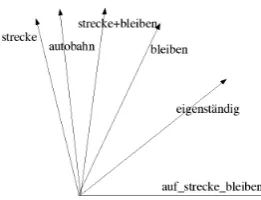
The comparisons we made are illustrated in Fig-ure 2, where vectors for the MWE auf die Strecke
bleiben ‘to fall by the wayside’ and the words Strecke ‘route’ and bleiben ‘to stay’ are mapped
5
Available as an example data collection in UCS-Toolkit 5 fromwww.collocations.de.
6For all our experiments we consider only two-word
com-binations.
7Schone & Jurafsky (2001) explore a few modest
Figure 2: Composed versus Multi-Word
into two dimensions8. (the words Autobahn ‘high-way’ and eigenst¨andig ‘independent’ are given for comparison). Here we see that the linear com-bination of the component words of the MWE is clearly distinct from that of the MWE as a whole.
As a further illustration of the difference be-tween the composed vector and the MWE vector, in Table 2 we list the words whose meaning vector is most similar to that of the MWE auf dis Strecke
[image:5.595.326.512.375.458.2]bleiben along with their similarity values, and in
Table 3 we list those words whose meaning vec-tor is most similar to the composed vecvec-tor. The semantic differences among these two classes are readily apparent.
folgerung ‘consequence’ 0.769663
eigenst¨andig ‘independent’ 0.732372
langfristiger ‘long-term’ 0.731411
herbeif¨uhren ‘to effect’ 0.717294
ausnahmef¨alle ‘exceptions’ 0.704939
Table 1: auf die Strecke bleiben
strecken ‘to lengthen’ 0.743309
fahren ‘to drive’ 0.741059
laufen ‘to run’ 0.726631
fahrt ‘drives’ 0.712352
[image:5.595.94.267.556.627.2]schließen ‘to close’ 0.704364
Table 2: Strecke+bleiben
We recognize that the composed vector is clearly nowhere near a perfect model of compo-sitional meaning in the general case. This can be illustrated by considering, for example, the MWE
fire breathing. This expression is clearly
com-positional, as it denotes the process of producing
8The preposition auf and the article die are on the stop list
combusting exhalation, exactly what the seman-tic combination rules of the English would pre-dict. Nevertheless the distribution of fire
breath-ing is quite unrelated to that of its constituents fire and breathing ( the former appears frequently
with dragon and circus while the later appear fre-quently with blaze and lungs, respectively). De-spite these principled objections, the composed vector provides a useful baseline for our investiga-tion. We should note that a number of researchers in the LSA tradition have attempted to provide more compelling combinatory functions to cap-ture the non-linearity of linguistic compositional interpretation (Kintsch, 2001; Widdows and Pe-ters, 2003).
As a check we chose, at random, a number of simple clearly-compositional word combinations (not from the candidate MWE list). We expected that on the whole these would evidence a very high similarity measure when compared with their as-sociated composed vector, and this is indeed the case, as shown in Table 1. We also compared
vor Gericht verantworten 0.80735103 ‘to appear in court’
im Bett liegen 0.76056000 ‘to lie in bed’
aus Gef¨angnis entlassen 0.66532673 ‘dismiss from prison’
Table 3: Non-idiomatic phrases
the literal and non-literal vectors for ins Wasser
fallen from the first experiment with the composed
vector, computed out of the meaning vectors for
Wasser and for fallen.9 The difference isn’t large, but nevertheless the composed vector is more sim-ilar to the literal vector (cosine of 0.2937) than to the non-literal vector (cosine of 0.1733).
Extending to the general case, our task was to compare the composed vector to the actual vec-tor for all the MWEs in our test set. The result-ing cosine similarity values range from 0.01 to 0.80. Our hope was that there would be a similar-ity threshold for distinguishing MWEs that have non-compositional interpretations from those that do not. Indeed of the MWEs with a similarity val-ues of under 0.1, just over half are MWEs which were hand-annotated to have non-literal uses.10 It
9
The preposition ins is on the stop list and plays no role in the computation.
is clear then that the technique described is, prima
facie, capable of detecting idiomatic MWEs.
3.3 Evaluation and Discussion
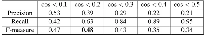
To evaluate the method, we used the careful man-ual annotation of the PNV database described by Krenn (2000) as our gold standard. By adopt-ing different threshholds for the classification de-cision, we obtained a range of results (trading off precision and recall). Table 4 illustrates this range. The F-score measure is maximized in our ex-periments by adopting a similarity threshold of 0.2. This means that MWEs which have a mean-ing vector whose cosine is under this value when compared with with the combined vector should be classified as having a non-literal meaning.
To compare our method with that proposed by Baldwin et al. (2003), we applied their method to our materials, generating LSA vectors for the component content words in our candidate MWEs and comparing their semantic similarity to the MWEs LSA vector as a whole, with the expecta-tion being that low similarity between the MWE as a whole and its component words is indication of the non-compositionality of the MWE. The results are given in Table 5.
It is clear that while Baldwin et al.’s expectation is borne out in the case of the constituent noun (the non-head), it is not in the case of the con-stituent verb (the head). Even in the case of the nouns, however, the results are, for the most part, markedly inferior to the results we achieved using the composed vectors.
There are a number of issues that complicate the workability of the unsupervised technique de-scribed here. We rely on there being enough non-compositional uses of an idiomatic MWE in the corpus that the overall meaning vector for the MWE reflects this usage. If the literal meaning is overwhelmingly frequent, this will reduce the effectivity of the method significantly. A second problem concerns the relationship between the lit-eral and the non-litlit-eral meaning. Our technique relies on these meaning being highly distinct. If the meanings are similar, it is likely that local con-text will be inadequate to distinguish a composi-tional from a non-composicomposi-tional use of the expres-sion. In our investigation it became apparent, in fact, that in the newspaper genre, highly idiomatic expressions such as ins Wasser fallen were often
Appendix I.
used in their idiomatic sense (apparently for hu-morous effect) particularly frequently in contexts in which elements of the literal meaning were also present.11
4 Conclusion
To summarize, in order to classify an MWE as non-compositional, we compute an approximation of its compositional meaning and compare this with the meaning of the expression as it is used on the whole. One of the obvious improvements to the algorithm could come from better mod-els for simulating compositional meaning. A fur-ther issue that can be explored is whefur-ther linguis-tic preprocessing would influence the results. We worked only on raw text data. There is some ev-idence (Baldwin et al., 2003) that part of speech tagging might improve results in this kind of task. We also only considered local word sequences. Certainly some recognition of the syntactic struc-ture would improve results. These are, however, more general issues associated with MWE pro-cessing.
Rather promising results were attained using only local context, however. Our study shows that the F-score measure is maximized by taking as threshold for distinguishing non-compositional phrases from compositional ones a cosine simi-larity value somewhere between 0.1-0.2. An im-portant point to be explored is that compositional-ity appears to come in degrees. As Bannard and Lascarides (2003) have noted, MWEs “do not fall cleanly into the binary classes of compositional and non-compositional expressions, but populate a continuum between the two extremes.” While our experiment was designed to classify MWEs, the technique described here, of course, provides a means, if rather a blunt one, for quantifying the degreee of compositonality of an expression.
References
Ricardo A. Baeza-Yates and Berthier A. Ribeiro-Neto. 1999. Modern Information Retrieval. ACM Press / Addison-Wesley.
Timothy Baldwin, Colin Bannard, Takaaki Tanaka, and Dominic Widdows. 2003. An empirical model
11
One such example from the SZ corpus:
Der Auftakt w¨are allerdings fast ins Wasser gefallen, weil ein geplatzter Hydrant eine f¨unfzehn Meter hohe Wasserfont¨ane in die Luft schleuderte.
cos<0.1 cos<0.2 cos<0.3 cos<0.4 cos<0.5
Precision 0.53 0.39 0.29 0.22 0.21
Recall 0.42 0.63 0.84 0.89 0.95
[image:7.595.131.467.62.121.2]F-measure 0.47 0.48 0.43 0.35 0.34
Table 4: Evaluation of Various Similarity Thresholds
cos<0.1 cos<0.2 cos<0.3 cos<0.4 cos<0.5
Verb F-measure 0.21 0.16 0.29 0.26 0.27
Noun F-measure 0.28 0.51 0.43 0.39 0.33
Table 5: Evaluation of Method of Baldwin et al. (2003)
of multiword expression decomposability. In
Pro-ceedings of the ACL-2003 Workshop on Multiword Expressions: Analysis, Acquisition and Treatment,
pages 89–96, Sapporo, Japan.
Colin Bannard, Timothy Baldwin, and Alex Las-carides. 2003. A statistical approach to the seman-tics of verb-particles. In Proceedings of the
ACL-2003 Workshop on Multiword Expressions: Analy-sis, Acquisition and Treatment, pages 65–72,
Sap-poro, Japan.
Michael W. Berry, Zlatko Drmavc, and Elisabeth R. Jessup. 1999. Matrices, vector spaces, and infor-mation retrieval. SIAM Review, 41(2):335–362.
Jean Carletta. 1996. Assessing agreement on classi-fication tasks: The kappa statistic. Computational
Linguistics, 22(2):249–254.
Scott Cederberg and Dominic Widdows. 2003. Using LSA and noun coordination information to improve the precision and recall of automatic hyponymy ex-traction. In In Seventh Conference on
Computa-tional Natural Language Learning, pages 111–118,
Edmonton, Canada, June.
Scott C. Deerwester, Susan T. Dumais, Thomas K. Lan-dauer, George W. Furnas, and Richard A. Harshman. 1990. Indexing by latent semantic analysis.
Jour-nal of the American Society of Information Science,
41(6):391–407.
Stefan Evert and Hannah Kermes. 2003. Experi-ments on candidate data for collocation extraction. In Companion Volume to the Proceedings of the 10th
Conference of The European Chapter of the Associ-ation for ComputAssoci-ational Linguistics, pages 83–86,
Budapest, Hungary.
Stefan Evert and Brigitte Krenn. 2001. Methods for the qualitative evaluation of lexical association mea-sures. In Proceedings of the 39th Annual Meeting
of the Association for Computational Linguistics,
pages 188–195, Toulouse, France.
Stefan Evert. 2004. The Statistics of Word
Cooccur-rences: Word Pairs and Collocations. Ph.D. thesis,
University of Stuttgart.
Christiane Fellbaum. 1998. WordNet, an electronic
lexical database. MIT Press, Cambridge, MA.
Nancy Ide and Jean V´eronis. 1998. Word sense dis-ambiguation: The state of the art. Computational
Linguistics, 14(1).
Walter Kintsch. 2001. Predication. Cognitive Science, 25(2):173–202.
Brigitte Krenn. 2000. The Usual Suspects: Data-Oriented Models for Identification and Representa-tion of Lexical CollocaRepresenta-tions. DissertaRepresenta-tions in
Com-putational Linguistics and Language Technology. German Research Center for Artificial Intelligence and Saarland University, Saarbr¨ucken, Germany.
Thomas K. Landauer and Susan T. Dumais. 1997. A solution to plato’s problem: The latent seman-tic analysis theory of the acquisition, induction, and representation of knowledge. Psychological Review, 104:211–240.
Thomas K. Landauer and Joseph Psotka. 2000. Sim-ulating text understanding for educational applica-tions with latent semantic analysis: Introduction to LSA. Interactive Learning Environments, 8(2):73– 86.
Dekang Lin. 1999. Automatic identification of non-compositional phrases. In Proceedings of the 37th
Annual Meeting of the Association for Computa-tional Linguistics, pages 317–324, College Park,
MD.
Christopher D. Manning and Hinrich Sch¨utze. 1999.
Foundations of Statistical NaturalLanguage Pro-cessing. The MIT Press, Cambridge, MA.
Ivan A. Sag, Timothy Baldwin, Francis Bond, Ann A. Copestake, and Dan Flickinger. 2002. Multiword expressions: A pain in the neck for NLP. In
Pro-ceedings of the 3rd International Conferences on Intelligent Text Processing and Computational Lin-guistics, pages 1–15.
of Empirical Methods in Natural Language Process-ing, Pittsburgh, PA.
Hinrich Sch¨utze. 1998. Automatic word sense dis-crimination. Computational Linguistics, 24(1):97– 124.
Bego˜na Villada Moir´on and J¨org Tiedemann. 2006. Identifying idiomatic expressions using automatic word-alignment. In Proceedings of the EACL 2006
Workshop on Multiword Expressions in a Multilin-gual Context, Trento, Italy.
Dominic Widdows and Stanley Peters. 2003. Word vectors and quantum logic: Experiments with nega-tion and disjuncnega-tion. In Eighth Mathematics of
Lan-guage Conference, pages 141–150, Bloomington,
Indiana.
Chengxiang Zhai. 1997. Exploiting context to iden-tify lexical atoms – a statistical view of linguistic context. In Proceedings of the International and
In-terdisciplinary Conference on Modelling and Using Context (CONTEXT-97), pages 119–129.
APPENDIX
Similarity (cosine) values for the combined and the MWE vector. Uppercase entries are those hand-annotated as being MWEs which have an id-iomatic interpretation.
Word Combinations Cosines
(vor) gericht verantworten 0.80735103
(in) bett liegen 0.76056000
(aus) gef¨angnis entlassen 0.66532673 (zu) verf¨uung stellen 0.60310321 (aus) haft entlassen 0.59105617 (um) prozent steigern 0.55889772
(ZU) KASSE BITTEN 0.526331
(auf) prozent sinken 0.51281725 (IN) TASCHE GREIFEN 0.49350031 (zu) verf¨ugung stehen 0.49236563 (auf) prozent steigen 0.47422122 (um) prozent zulegen 0.47329672 (in) betrieb gehen 0.47262171 (unter) druck geraten 0.44377297 (in) deutschland leben 0.44226071 (um) prozent steigen 0.41498688 (in) rechnung stellen 0.40985534 (von) prozent erreichen 0.39407666 (auf) markt kommen 0.38740534 (unter) druck setzen 0.37822936 (in) vergessenheit geraten 0.36654168 (um) prozent sinken 0.36600216
(in) rente gehen 0.36272313
(zu) einsatz kommen 0.3562527 (zu) schule gehen 0.35595884 (in) frage stellen 0.35406327 (in) frage kommen 0.34714701 (in) luft sprengen 0.34241143 (ZU) GESICHT BEKOMMEN 0.34160325 (vor) gericht ziehen 0.33405685
(in) gang setzen 0.33231573
(in) anspruch nehmen 0.32217044 (auf) prozent erh¨ohen 0.31574088 (um) prozent wachsen 0.3151615 (in) empfang nehmen 0.31420746 (f¨ur) sicherheit sorgen 0.30230156
(zu) ausdruck bringen 0.30001438 (IM) MITTELPUNKT STEHEN 0.29770654
(zu) ruhe kommen 0.29753093
(IM) AUGE BEHALTEN 0.2969367 (in) urlaub fahren 0.29627064
(in) kauf nehmen 0.2947628
(in) pflicht nehmen 0.29470704 (in) h¨ohe treiben 0.29450525 (in) kraft treten 0.29311349 (zu) kenntnis nehmen 0.28969961
(an) start gehen 0.28315812
(auf) markt bringen 0.2800427 (in) ruhe standgehen 0.27575604 (bei) prozent liegen 0.27287073 (um) prozent senken 0.26506203 (UNTER) LUPE NEHMEN 0.2607078
(zu) zug kommen 0.25663165
(zu) ende bringen 0.25210009 (in) brand geraten 0.24819525 ( ¨UBER) B ¨UHNE GEHEN 0.24644366 (um) prozent erh¨ohen 0.24058016 (auf) tisch legen 0.23264335 (auf) b¨uhne stehen 0.23136641 (auf) idee kommen 0.23097735
(zu) ende gehen 0.20237252
(auf) spiel setzen 0.20112171 (IM) VORDERGRUND STEHEN 0.18957473 (IN) LEERE LAUFEN 0.18390151 (zu) opfer fallen 0.17724105 (in) gefahr geraten 0.17454816 (in) angriff nehmen 0.1643926 (auer) kontrolle geraten 0.16212899
(IN) HAND NEHMEN 0.15916243
(in) szene setzen 0.15766861 (ZU) SEITE STEHEN 0.14135151 (zu) geltung kommen 0.13119923 (in) geschichte eingehen 0.12458956 (aus) ruhe bringen 0.10973377 (zu) fall bringen 0.10900036
(zu) wehr setzen 0.10652383
(in) griff bekommen 0.10359659 (auf) tisch liegen 0.10011075 (IN) LICHTER SCHEINEN 0.08507655 (zu) sprache kommen 0.08503791
(IM) STICH LASSEN 0.0735844
(unter) beweis stellen 0.06064519
(IM) WEG STEHEN 0.05174435
(AUS) FUGEN GERATEN 0.05103952 (in) erinnerung bleiben 0.04339438
(ZU) WORT KOMMEN 0.03808749