Attentive Language Models
Giancarlo D. Salton and Robert J. Ross and John D. Kelleher
Applied Intelligence Research Centre School of Computing
Dublin Institute of Technology Ireland
[email protected] {robert.ross,john.d.kelleher}@dit.ie
Abstract
In this paper, we extend Recurrent Neural Network Language Models (RNN-LMs) with an attention mechanism. We show that an Attentive RNN-LM (with 14.5M parameters) achieves a better perplexity than larger RNN-LMs (with 66M param-eters) and achieves performance compa-rable to an ensemble of 10 similar sized RNN-LMs. We also show that anAttentive RNN-LM needs less contextual informa-tion to achieve similar results to the state-of-the-art on the wikitext2 dataset.
1 Introduction
Language Models (LMs) are an essential compo-nent in a range of Natural Language Processing applications, such as Statistical Machine Trans-lation and Speech Recognition (Schwenk et al., 2012). An LM provides a probability for a se-quence of words in a given language, reflecting fluency and the likelihood of that word sequence occurring in that language.
In recent years Recurrent Neural Networks (RNNs) have improved the state-of-the-art in LM research (J´ozefowicz et al.,2016). Sequential data prediction, however, is still considered a challenge in Artificial Intelligence (Mikolov et al., 2010) given that, in general, prediction accuracy de-grades as the size of sequences increase.
RNN-LMs sequentially propagate forward a context vector by integrating the information gen-erated by each prediction step into the context used for the next prediction. One consequence of this forward propagation of information is that older information tends to fade from the context as new information is integrated into the context. As a re-sult, RNN-LMs struggle in situations where there is a long-distance dependency because the relevant
information from the start of the dependency has faded by the time the model has spanned the de-pendency. A second problem is that the context can be dominated by the more recent information so when an RNN-LM does make an error this error can be propagated forward resulting in a cascade of errors through the rest of the sequence.
In recent sequence-to-sequence research the concept of “attention” has been developed to en-able RNNs to align different parts of the input and output sequences. Examples of attention based architectures include Neural Machine Translation (NMT) (Bahdanau et al.,2015;Luong et al.,2015) and image captioning (Xu et al.,2015).
In this paper we extend the RNN-LM context mechanism with an attention mechanism that en-ables the model to bring forward context infor-mation from different points in the context se-quence history. We hypothesis that this atten-tion mechanism enables RNN-LMs to: (a) bridge long-distance dependencies, thereby avoiding er-rors; and, (b) to overlook recent errors by choos-ing to focus on contextual information precedchoos-ing the error, thereby avoiding error propagation.
We show that a medium sized1 Attentive
RNN-LM2 achieves better performance than larger
“standard” models and performance comparable to an ensemble of 10 “medium” sized LSTM RNN-LMs on the PTB. We also show that an At-tentive RNN-LM needs less contextual informa-tion in order to achieve similar results to state-of-the-art results over the wikitext2 dataset.
Outline: §2introduces RNN-LMs and related research, §3 outlines our approach, §4 describes our experiments, §5 presents our analysis of the models‘ performance and§6our conclusions.
1We adopt the terminology ofZaremba et al.(2015) and
Press and Wolf(2016) when referring to the size of the RNNs. 2Code available at https://github.com/ giancds/attentive_lm
2 RNN-Language Models
RNN-LMs model the probability of a sequence of words by modelling the joint probability of the words in the sequence using the chain rule:
p(w1, . . . , wN) = N Y
t=1
p(wn|w1, . . . , wn−1) (1)
whereN is the number of words in the sequence. The context of the word sequence is modelled by an RNN and for each position in the sequence the probability distribution over the vocabulary is calculated using a softmax on the output related to that position of the RNN‘s last layer (i.e., the last layer‘s hidden state) (J´ozefowicz et al.,2016). Examples of such models include Zaremba et al. (2015) and Press and Wolf (2016). These mod-els are composed of LSTM units (Hochreiter and Schmidhuber, 1997) and apply regularization to improve the RNN performance. In addition,Press and Wolf (2016) also uses the same embedding matrix that is used to transform the input words to transform the output of the last RNN layer to feed it to the softmax layer to make the next prediction. Attention mechanisms were first proposed in “encoder-decoder” architectures for NMT sys-tems. Bahdanau et al. (2015) proposed a model that stores all the encoder RNN’s outputs and uses them together with the decoder RNN’s stateht−1
to compute a context vector that, in turn, is used to compute the state ht. In Luong et al. (2015) a generalization of the model of Bahdanau et al. (2015) is presented which uses the decoder RNN‘s state, in this instance ht rather than ht−1, along
with the outputs of the encoder RNN to compute a context vector that it then concatenated withht before making the next prediction. Both models have similar performance and achieve state-of-the-art performance for some language pairs; how-ever, they suffer from repeating words or dropping translations at the output (Mi et al.,2016).
There is previous work on using past informa-tion to improve RNN-LMs.Tran et al.(2016) pro-pose an extension to LSTM cells to include mem-ory areas, which depend on input words, at the output of every hidden layer. The model produces good results but the dependency on input words expands the number of parameters in each LSTM cell in proportion to the vocabulary size in use.
Similarly, Cheng et al. (2016) propose storing the LSTM‘s memory cells of every layer at each timestep and draw a context vector for each mem-ory cell for each new input to attend to previous content and compute its output. Although their model requires fewer parameters than the model of Tran et al.(2016), the performance of the model is worse than regularized “standard” RNN-LM as in Zaremba et al.(2015) andPress and Wolf(2016).
Daniluk et al.(2017) propose an augmented ver-sion of the attention mechanism proposed by Bah-danau et al.(2015) on which their model outputs 3 vectors calledkey-value-predict. Thekey(a vector of real numbers) is used to retrieve a single hidden state from the past.Grave et al.(2017) propose an LM augmented with a “memory cache” that stores tuples of hidden-states plus word embeddings (for the word predicted from that hidden state). The memory cache is used to help the current predic-tion by retrieving the word embedding associated with the hidden state in the memory most similar to the current hidden state. Merity et al. (2017) proposed a mixture model that includes an RNN and a pointer network. This model computes one distribution for the softmax component and one distribution for the pointer network, using a sen-tinel gating function to combine both distributions. In spite of the fact that their model is similar to the model ofGrave et al.(2017), their model requires an extra transformation between the current state of the RNN and those stored in the memory.
These recent models have a number of draw-backs. The systems that extend the architecture of LSTM units struggle to process large vocabularies because the system memory expands to the size of the vocabulary. For systems that retrieve a single hidden-state or word from memory, if the predic-tion is not correct, the RNN-LM will not receive the correct past information. Finally, the models of Merity et al. (2017) and Grave et al. (2017) use a fixed-length memory ofL previous hidden states to store and retrieve information from the past (100 states in the case ofMerity et al.(2017) and 2,000 states in the case ofGrave et al.(2017)). As we shall explain in §3 our “attentive” RNN-LMs have a memory of dynamic-length that grows with the length of the input and therefore, in gen-eral, are computationally cheaper.
RNN-LM to represent previous input words and we use a set of attention weights (instead of a key) to retrieve information from the past inputs. The main advantages of our approach are: (a) our model does not need vocabulary sized matrices in the computations of the attention mechanism and therefore has a reduced number of parame-ters; and (b) as we use all previous hidden states of the RNN-LM in the computation for the atten-tion weights, all of those states will influence the next prediction based on the weights calculated.
3 Attentive Language Models
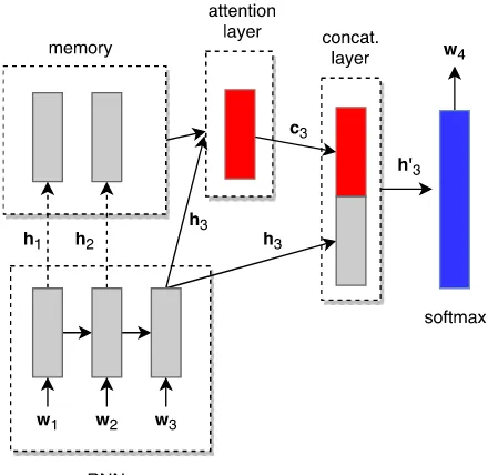
In this work we extend RNN-LMs to include an at-tention mechanism over previous inputs. We em-ploy a multi-layered RNN to encode the input and, at each timestep, we store the output of the last re-current layer (i.e., its hidden stateht) into a mem-ory buffer. We compute a score for each hidden statehi (∀i ∈ {1, . . . , t−1}) stored in memory and use these scores to weight eachhi. From these weighted hidden states we generate a context vec-torctthat is concatenated with the current hidden stateht to predict the next word in the sequence. Figure1illustrates a step of our model when pre-dicting the fourth word in a sequence.
We propose two different attention score func-tions that can be used to compute the context vector ct. One calculates the attention score of each hi using just the information in the state (the single(hi) score introduced below). The other calculates the attention scores for each hi by combining the information from that state with the information from the current state ht (the
combined(hi,ht) score described below). Each of these mechanisms defines a separateAttentive RNN-LMs and we report results for each of these LMs in our experiments.
More formally, eachhtis computed as follows, wherextis the input at timestept:
ht=RNN(xt,ht−1) (2)
The context vector ct is then generated using Eq. (3) where each scalar weight ai is a softmax (Eq. (4)) and the score for each hidden state (hi) in the memory buffer is one of Eq. (5) or Eq. (6).
ct= t−1
X
i=1
[image:3.595.306.526.62.276.2]aihi (3)
Figure 1: Illustration of a step of the Attentive RNN-LM withcombinedscore. In this example, the model receives the third word as input (w3)
af-ter storing the previous states (h1andh2) in
mem-ory. After producingh3, the model computes the
context vector (in this case c3) that will be
con-catenated to h3 before the softmax layer for the
prediction of the fourth wordw4. Note that if the
single score is in use (Eq. (9)), the arrow from the RNN output for h3 to the attention layer is
dropped. Also note that h3 is stored in memory
only at the end of this process.
ai= Pt−1exp(score(hi,ht))
j=1exp(score(hj,ht)) (4)
score(hi,ht) =
single(h
i) (5)
combined(hi,ht) (6) We then mergectwith the current statehtusing a concatenation layer3, where Wc is a matrix of
parameters andbtis a bias vector.
h0
t=tanh(Wc[ht;ct] +bt) (7)
We compute the next word probability using Eq.8 where W is a matrix of parameters and b
is a bias vector.
3We also have experimented with using a dot product and a feedforward layer to combinehtandctand also using only
p(wt|w<t, x) =softmax(Wh0t+b) (8)
Singlescore. This score is calculated for each
hi using just the information stored the state in it-self. The scoresingle(hi)is defined as
single(hi) =vstanh(Wshi) (9)
where the parameter matrixWsand vectorvsare both learned by the attention mechanism and represents the dot product.
When applying the single(hi) score, we can think of the score ai as a scalar summary of the “absolute relevance” of the statehi. When a new stateht is added to the buffer its scalar summary
aiis calculated by first using Eq.9to get the score for the state and then applying a softmax func-tion over the set of state scores including the score for the new state. Although the scores for each state do not change from one timestep to the next, applying the softmax results in recalculation of the distribution of the scalar summaries for all the statesh0, . . . ,ht. As a result theai’s for each state in Eq.3changes from one prediction to the next as new states are added and the weight mass is dis-tributed across more states.
Combined score. This score is calculated for each hi by combining the information from that state with the information from the current state
ht. The scorecombined(hi,ht)is defined as
combined(hi,ht) =vstanh(Wshi+Wqht) (10)
where the parameter matrices Ws and Wq and vectorvsare learned by the attention mechanism, andis the same as in Eq.9. Notice that because
Wqht does not depend on any other state and is used in the computations with all otherhi, we can efficiently compute it once and use the results in Eq.10, thus reducing computation time.
The scoreai defined bycombined(hi,ht), can be understood as the “relative relevance” of state
hi to the current state ht. Using this attention mechanism the score for each hi is different for each timestep according to its relevance to the cur-rent hidden statehtof the RNN. Consequently, the
scores for eachhi and the distribution over these scores changes from one timestep to the next. Us-ing this scorUs-ing, the model can decide whether it should pay more attention to the current state, to a previous state or use past states to “supplement” the information for the next prediction. In§5we present and analysis of how the model attends to different parts of its history as it generates a se-quence of predictions.
4 Experiments
To evaluate ourAttentiveRNN-LMs we conducted experiments over the PTB (Marcus et al., 1994) and wikitext2 (Merity et al., 2017) datasets. We first describe the setup of ourAttentiveRNN-LM for the PTB (§4.1) and wikitext2 (§4.2) datasets and then discuss the results (§4.3). We com-pare our results on PTB toZaremba et al. (2015) and Press and Wolf (2016) the best performing LSTM-LMs on the PTB, two memory augmented networks (Grave et al. (2017) and Merity et al. (2017)) and PTB state-of-the-art ensemble mod-els ofZaremba et al.(2015). On wikitext2 we take (Merity et al., 2017), the creators of the dataset, and (Grave et al., 2017), the current state-of-the-art, as our baselines.
4.1 PTB Setup
We evaluate ourAttentiveRNN-LM over the PTB dataset using the standard split which consists of 887K, 70K and 78K tokens on the training, vali-dation and test sets respectively.
con-nections and clip the norm of the gradients, nor-malized by mini-batch size, at 5.0. In all our ex-periments, we followPress and Wolf (2016) and tie the matrixW in Eq. (8) to be the embedding matrix (which also has 650 dimensions) used to represent the input words.
Contrary toZaremba et al.(2015) andPress and Wolf (2016), we do not allow successive mini-batches to sequentially traverse the dataset. In other words, we follow the standard practice to reinitialize the hidden state of the network at the beginning of each mini-batch, by setting it to all zeros. This way, we do not allow the attention window to span across sentence boundaries4. We
use all sentences in the training set, we truncate all sentences longer than 35 words and pad all sen-tences shorter than 35 words with a special symbol so all sentences are the same size. We use a vo-cabulary size of 10K words and a batch size of 32. All UNK words (following the pre-processing of (2015)) were kept during the training, validation and testing phases.
4.2 wikitext2 Setup
We also evaluate ourAttentiveRNN-LM over the wikitext2 dataset (Merity et al.,2017). We use the standard train, validation and test splits which con-sists of around 2M, 217K tokens and 245k tokens respectively. This dataset is composed of “Good” and “Featured” articles on Wikipedia.
There is an important difference between how we trained and tested our models on the wiki-text2 dataset and how the baseline systems were trained and tested. BothMerity et al.(2017) and Grave et al.(2017) permitted the memory buffers of their systems to span sentence boundaries (and, indeed, they also did mini-batch traversal which allowed the memory buffers to traverse mini-batch boundaries) whereas we reset our systems mem-ory at each sentence boundary. This difference is important because in the wikitext2 dataset the sentences are not shuffled and, therefore, are se-quentially related to each other. As a result, sys-tems that carry sequential information from pre-vious sentences into the current sentence have an advantage in that they utilise contextual cues from the preceding sentence to inform the predictions at the start of the new sentence. By
compari-4We also experimented to with successive mini-batches to sequentially traverse the dataset as inZaremba et al.(2015) but the performance of the model dropped considerably so we do not report those results here.
son, systems that reset their memory at the start of each sentence must reconstruct their context mod-els from scratch and face a “cold-start” problem for the early predictions in the sentence.
The core reason why (Merity et al.,2017) and (Grave et al., 2017) did not reset their memo-ries across sentence boundamemo-ries and we do is that these baseline systems use a fixed length memory whereas our “attention” mechanism has a variable length memory. A variable length memory has benefits in terms of both computational cost and the fact that the memory size is dynamically fitted to the context. However, just as the system de-signer for a fixed length memory LM must fix the memory size hyper-parameter in some fashion, so to the designer of a variable length memory LM must decide when the memory buffer is reset. For our work, we have decided to reset our memory buffer at sentence boundaries because many of the tasks for which LMs are used (e.g. NMT) work on a sentence by sentence basis. If required it would be possible for us to extend the memory buffer to the start of the preceding sentence (or some other landmark is the sequence history). However, this would incur extra computational cost, and as we shall see ourAttentiveRNN-LMs are still compet-itive on the wikitext2 dataset despite the fact that the baselines systems are given access to longer context sequences.
We trained an Attentive RNN-LM with 2 lay-ers of 1000 LSTM units using Stochastic Gradient Descent (SGD) with an initial learning rate of 1.0, decaying the learning rate by a factor of 1.15 at each epoch after 14 epochs, to minimize the aver-age negative log probability of the target words.
Similarly to the PTB model we also train this model with an early stop counter of 10 epochs and we initialize the weight matrices of the net-work uniformly in [−0.05,0.05] while all biases are initialized to a constant value at0.0. We apply
65%dropout to the non-recurrent connections and clip the norm of the gradients, normalized by mini-batch size, at5.0. In all our experiments, we also follow Press and Wolf (2016) and tie the matrix
33,278 and a batch size of 32. All UNK words (following the pre-processing of (2017)) were kept during the training, validation and testing phases. 4.3 Results
In Table1we report the results of our experiments on the PTB dataset. As we can see in this table, theAttentiveRNN-LMs outperforms all other sin-gle models on the PTB dataset. Although Atten-tive RNN-LMs have less parameters (10M) than the large “regularized” LSTM-LMs (66M param-eters), they were capable of reducing the perplex-ity over both validation and test sets. This result shows that using anAttentiveRNN-LM it is pos-sible to achieve better perplexity scores with far fewer model parameters. Furthermore, Attentive RNN-LMs are able to achieve roughly the same results as the averaging of 10 RNN-LM models (with no attention) of the same size.
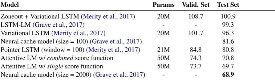
In addition, there is little difference between the results of theAttentiveRNN-LM withsinglescore (Eq.9) and theAttentiveRNN-LM withcombined score (Eq.10) with thesinglescore slightly outper-forming the the combinedscore. We believe this is because the model using thecombined(hi,ht) score has more parameters to optimize and, thus, more difficulties in settling to a good local optima. In Table2we report the results on the wikitext2 dataset. Despite the fact that we reset the mem-ory for the Attentive RNN-LM at each sentence boundary whereas the caches for the baseline sys-tems span sentence boundaries, our bestAttentive RNN-LM is within 1 perplexity point of the sys-tem of (2017) (which is allowed to cache 2,000 previous hidden states), and has a lower perplexity than all of the other baselines.
5 Analysis of the Models
The purpose of our attention mechanism is to en-able an RNN-LM to bridge long distance depen-dencies in language. Therefore, we expect the at-tention mechanism to select previous hidden states that are relevant to the current predictions. To analyse whether the attention mechanism is func-tioning as intend we analysed the evolution of at-tention weights in ourAttentive RNN-LM as we calculated the perplexity for samples sentences us-ing the models trained over the wikitext25.
5The behaviour of the models on wikitext2 is similar to that of the models trained and evaluated on the PTB dataset, so for space reasons we only present the wikitext2 analysis here.
Figure 2 show the evolution of attention weights, using both single and combined scoring, when calculating perplexities for 2 sentences con-taining nominal modifiers. In addition, Figure 3 show the evolution of attention weights for two sentences containing relative clauses, once again using both single and combined scoring. The words in the X-axis (horizontal) are the inputs at each timestep and the words in the Y-axis (verti-cal) are the next (or predicted) words. We sup-pressed weights that either equal to 1.0 (black squares) or 0.0 (white squares). Note that given the rounding to 4 decimal places, weights in some rows of the matrices may not sum to1.0.
None of the attention mechanisms worked as a proper attention mechanism. In other words, none of the mechanisms generated larger weights for specific words in the sentence, in comparison to the other words in the same sentence. Compar-ing the attention weights generated by both com-binedscore andsinglescore for both sentences, it is striking that the distribution of attention weights is very similar. For bothAttentiveRNN-LM mod-els the attention spreads out across the history in a relatively equal fashion.
Indeed, both models seem to take into consid-eration all previous states, creating a smoothing effect for the hidden states in the buffer. There-fore, no single state dominates the context vector by receiving a much larger attention weight than the others. We believe that this behaviour enables the models to bring forward information from the beginning of the sentence at the time it is making a prediction. This way, the models do not let infor-mation fade away from the context as it progresses to subsequent steps in a sequence and all previ-ous information about the words that preceded the current timestep is available to the classifier in a manner that disregards recency.
Model Params Valid. Set Test Set Single Models
Medium Regularized LSTM (Zaremba et al.,2015) 20M 86.2 82.7 Large Regularized LSTM (Zaremba et al.,2015) 66M 82.2 78.4 Large + BD + WT (Press and Wolf,2016) 51M 75.8 73.2 Neural cache model (size = 500) (Grave et al.,2017) - - 72.1 Medium Pointer Sentinel-LSTM (Merity et al.,2017) 21M 72.4 70.9 Attentive LM w/combinedscore function 14.5M 72.6 70.7 Attentive LM w/singlescore function 14.5M 71.7 70.1 Model Averaging
[image:7.595.76.527.64.310.2]2 Medium regularized LSTMs (Zaremba et al.,2015) 40M 80.6 77.0 5 Medium regularized LSTMs (Zaremba et al.,2015) 100M 76.7 73.3 10 Medium regularized LSTMs (Zaremba et al.,2015) 200M 75.2 72.0 2 Large regularized LSTMs (Zaremba et al.,2015) 122M 76.9 73.6 10 Large regularized LSTMs (Zaremba et al.,2015) 660M 72.8 69.5 38 Large regularized LSTMs (Zaremba et al.,2015) 2508M 71.9 68.7
Table 1: Perplexity results over the PTB. Symbols: WT = weight tying (Press and Wolf,2016); WD = weight decay and BD = Bayesian Dropout, both suggested byGal and Ghahramani(2015).
Model Params Valid. Set Test Set
Zoneout + Variational LSTM (Merity et al.,2017) 20M 108.7 100.9
LSTM-LM (Grave et al.,2017) - - 99.3
Variational LSTM (Merity et al.,2017) 20M 101.7 96.3 Neural cache model (size = 100) (Grave et al.,2017) - - 81.6 Pointer LSTM (window = 100) (Merity et al.,2017) 21M 84.8 80.8 Attentive LM w/combinedscore function 50M 74.3 70.8 Attentive LM w/singlescore function 50M 73.7 69.7 Neural cache model (size = 2000) (Grave et al.,2017) - - 68.9
Table 2: Perplexity results over the wikitext2.
Another interpretation of thesmoothing effectis that it “reinforces” the signal in a similar fashion to residual connections in other RNNs and Deep Neural Networks architectures. Other RNN archi-tectures use these residual connections as a short-cut to “reinforce” the signal of the current input and, thus, it still considers the current input only. TheAttentiveRNN-LM, however, uses all the pre-vious hidden states to achieve a similar effect and create a stronger signal to the softmax classifier.
6 Conclusions
This paper proposes the use of attention mecha-nisms in RNN-LMs. These attention mechamecha-nisms enable an RNN-LM to consider information from its past when it is predicting the next word. We believe that this can help the LM to overcome
the fading of relevant information as it traverses a long-distance dependency within a sequence and also to recover from a mistaken prediction by fo-cusing on the context preceding the error.
Our results show that an Attentive RNN-LM outperforms both RNN-LM models that use and that do not use past information to predict the next word in a sequence when trained on the PTB dataset. Furthermore, ourAttentiveRNN-LM achieves this performance using far fewer units than the “standard” RNN-LM and, therefore, less model parameters. Our results also show that our Attentive RNN-LM achieves similar results to an ensemble that averages over 10 similar sized (in terms of number of LSTM units) RNN-LMs.
[image:7.595.77.524.354.486.2]state-of-the-art results over the wikitext2 dataset. It is an inter-esting result given that we do not allow our model to look beyond the boundaries of the current se-quence it is processing, whilst the state-of-the-art model is allowed to store 2,000 previous states in its cache.
In future work we plan to (a) test the perfor-mance of ensembles of Attentive RNN-LMs and (b) to study the use of theAttentive RNN-LM as the decoder within an NMT system.
Acknowledgments
This research was partly funded by the ADAPT Centre. The ADAPT Centre is funded un-der the SFI Research Centres Programme (Grant 13/RC/2106) and is co-funded under the European Regional Development Fund. Giancarlo D. Salton would like to thank CAPES (“Coordenac¸˜ao de Aperfeic¸oamento de Pessoal de N´ıvel Superior”) for his Science Without Borders scholarship, proc n. 9050-13-2.
References
Dzmitry Bahdanau, Kyunghyun Cho, and Yoshua Ben-gio. 2015. Neural machine translation by jointly
learning to align and translate. In International
Conference on Learning Representations, volume abs/1409.0473v6.
Jianpeng Cheng, Li Dong, and Mirella Lapata. 2016. Long short-term memory-networks for machine
reading. InProceedings of the 2016 Conference on
Empirical Methods in Natural Language Process-ing, pages 551–561, Austin, Texas. Association for Computational Linguistics.
Michal Daniluk, Tim Rockt¨aschel, Johannes Welbl, and Sebastian Riedel. 2017. Frustratingly Short
At-tention Spans in Neural Language Modeling. 5th
International Conference on Learning Representa-tions (ICLR’2017).
Yarin Gal and Zoubin Ghahramani. 2015. A theoret-ically grounded application of dropout in recurrent neural networks.
Edouard Grave, Armand Joulin, and Nicolas Usunier. 2017. Improving neural language models with a
continuous cache. 5th International Conference on
Learning Representations (ICLR’2017).
Sepp Hochreiter and J¨urgen Schmidhuber. 1997. Long short-term memory. volume 9, pages 1735–1780. Rafal J´ozefowicz, Oriol Vinyals, Mike Schuster, Noam
Shazeer, and Yonghui Wu. 2016. Exploring the lim-its of language modeling.
Minh-Thang Luong, Hieu Pham, and Christopher D. Manning. 2015. Effective approaches to attention-based neural machine translation. InProceedings of the 2015 Conference on Empirical Methods in Nat-ural Language Processing, pages 1412–1421.
Mitchell Marcus, Grace Kim, Mary Ann
Marcinkiewicz, Robert MacIntyre, Ann Bies, Mark Ferguson, Karen Katz, and Britta
Schas-berger. 1994. The penn treebank: Annotating
predicate argument structure. InProceedings of the Workshop on Human Language Technology, pages 114–119.
Stephen Merity, Caiming Xiong, James Bradbury, and Richard Socher. 2017. Pointer sentinel mixture
models. 5th International Conference on Learning
Representations (ICLR’2017).
Haitao Mi, Baskaran Sankaran, Zhiguo Wang, and Abe
Ittycheriah. 2016. Coverage embedding models for
neural machine translation. InProceedings of the 2016 Conference on Empirical Methods in Natu-ral Language Processing, pages 955–960, Austin, Texas. Association for Computational Linguistics. Tomas Mikolov, Martin Karafi´at, Luk´as Burget, Jan
Cernock´y, and Sanjeev Khudanpur. 2010.
Recur-rent neural network based language model. In
IN-TERSPEECH 2010, 11th Annual Conference of the International Speech Communication Association, Makuhari, Chiba, Japan, September 26-30, 2010, pages 1045–1048.
Ofir Press and Lior Wolf. 2016. Using the output embedding to improve language models. volume abs/1608.05859.
Holger Schwenk, Anthony Rousseau, and Mohammed Attik. 2012. Large, pruned or continuous space lan-guage models on a gpu for statistical machine
trans-lation. In Proceedings of the NAACL-HLT 2012
Workshop: Will We Ever Really Replace the N-gram Model? On the Future of Language Modeling for
HLT, pages 11–19.
Nitish Srivastava, Geoffrey Hinton, Alex Krizhevsky, Ilya Sutskever, and Ruslan Salakhutdinov. 2014.
Dropout: A simple way to prevent neural networks from overfitting. Journal of Machine Learning Re-search, 15:1929–1958.
Ke M. Tran, Arianna Bisazza, and Christof Monz. 2016. Recurrent memory network for language
modeling. arXiv, abs/1601.01272.
Kelvin Xu, Jimmy Ba, Ryan Kiros, Kyunghyun Cho, Aaron Courville, Ruslan Salakhudinov, Rich Zemel, and Yoshua Bengio. 2015. Show, attend and tell: Neural image caption generation with visual
atten-tion. In Proceedings of the 32nd International
Conference on Machine Learning (ICML-15), pages 2048–2057.