An Algorithm for Determining Talker Location using a Linear Microphone Array and Optimal Hyperbolic Fit

(1)

An Algorithm for Determining Talker

Location using a Linear Microphone

Array and Optimal Hyperbolic Fit

Harvey F. Silverman

Laboratory for Engineering Man/Machine Systems (LEMS) Division of Engineering

Brown University Providence, RI 02912

Abstract

One of the problems for all speech input is the necessity for the talker to be encumbered by a head. mounted, hand-held, or fixed position microphone. An intelfigent, electronically-aimed unidirectional microphone would overcome this problem. Array techniques hold the best promise to bring such a system to practicality. The development of a robust algorithm to determine the location of a talker is a fundamental is- sue for a microphone-array system. Here, a two-step talker-location algorithm is introduced. Step 1 is a rather conventional filtered cross-correlation method; the cross-correlation between some pair of microphones is determined to high accuracy using a some- what novel, fast interpolation on the sampled data. Then, using the fact that the delays for a point source should fit a hyperbola, a best hyperbolic fit is obtained using nonlinear optimization. A method which fits the hyperbola directly to peak-picked delays is shown to be far less robust than an algorithm which fits the hyperbola in the cross-correlation space. An efficient, global nonlinear optimization technique, Stochastic region Contraction (SRC) is shown to yield highly accurate (>90%), and computationally efficient, results for a normal ambient.

Introduction

One of the problems for all speech input is the necessity for the talker to be encumbered by a hcad- mounted, hand-held, or fixed position microphone, or, perhaps, a technician-conlxolled mechanical unidirectional microphone. Whether for teleconferencing [I], speech recognition [2], or large-room recording or conferencing [3], an intelligent, eleclronically-aimed unidirectional microphone would overcome this problem. Array techniques hold the best promise to bring such a system to practicality.

Algorithms for passive tracking -- the determina- tion of range, bearing, speed, and signature as a function of time for a moving object -- have been studied for nearly 100 years partiomLqrly for radar and sonar systems. While there is currently much activity involved with the wacking of multiple sources using variants of the eigenvalue-hased decomposition MUSIC algorithm, [4], [5], [6], [7], [8], most systems still use correlational techniques

[9], [10], [11].

The method presented here is also based on correlation. First, a coarse, normalized cross-correlation function is computed over the delay range of interest. It turns out that, even for the relatively high sampfing rate of 20kHz, the 5Olas resolution of the time-delay estimates causes derived locations to be unsatisfactory. However, the latter may be refined by nearly two orders of magnitude through accurate interpolation techniques which can be attained for a relatively small computational using multirate filtering[12].

For M microphones, one can estimate M-1 independent relative delays. As, theoretically, only two relative delays are needed to triangulate a source, for M >3, the system is overspecified. However, since noise is always present in a real system, this extra information can be profitably used to overcome some of the effects of the noise. In fact, the geometry of the array constrains the vector of relative delays. For example, a simple linear array, with all the microphones on the axis, y=0, has delays constrained to be on a particular hyperbola with a focus on the target. Therefore, errors in the estimation of the delays may be corrected by fitting the best hyperbola. Two methods for doing so are presented here.

(2)

often "dumb" errors.

TDEHF

is introduced in Section 4. The second (and more robust) method Interpolated

Cross-eorrelation Hyperbolic Fit (ICHF), fits the best

hyperbola to the actual output of the interpolated cross-

correlations. As reasonable crosscorrelations

are

always

positive, the sum of the crosscorrelations across all the

microphones for

a

given hyperbola is used

as

a functional

to maximize. As

the

functional surface is multimodal,

results for a hierarchical grid search and for application of

Stochastic Region Contraction (SRC), [14]

,

[IS], a new

method for efficient global nonlinear optimization,

are

presented.

Coarse Cross-Correlation

Consider

a

linear microphone array having M mi-

crophones, each located on the line y = O at a distinct

point (z,,O) in the x y plane. A simple case is to be

considered in this paper in which a single some (talker) is located at some point (x,y) in frdnt of the array. although there will be ambient noise. Without loss of

generality, microphone 1 is selected

as

the reference. It

is assumed that the signal at each microphone is appropri-

ately sampled at some reasonable rate, R and that each

microphone thus receives a signal of time (indexed by j).

p:~). As sources might be separable in

the

frequency

domain, one

can,

in general, filter each received signal

using a zero-phase FIR filter, this is

the

only reasonable

choice

as

delay estimation is yet to be performed. This

implies,

where

f , G )

is a 2J+1 element symmetric FIR filter. It

is advantageous, as will be seen later, to define

rectangularly-windowed data, referenced to time index k',

for the correlations

as,

O I I I L - 1

otherwise (2.2)

Each of

the

M-1 independent cross-correlations for

a

delay of k samples each of duration 1IR may be

defined,

A,(k') L-1

C:[k,k'I

7

x r : (k '+l )$(k'+l +k), (2.3)

L

-

lkl

where A,(k') is a normalizing factor. A reasonable nor-

malization is to make the autocorrelation of

the

unshifted

reference signal have a value of unity for any particular

time reference k

',

Combining (2.3) and (2.4) gives,

which generalizes to,

Computational Considerations for the Cross-

Correlations

An important consideration is the selection of L.

the number of points in the crosscorrelation. When auto-

correlations are taken for

LPC

analysis, the length is lim-

ited by the assumption that the vocal tract is essentially

stationary over the interval. As one is not doing this pseudo-stationary modeling of the vocal tract, this fact

does not limit L here. Rather, the tradeoff

between

infor-

mation

content

-

tending to make one increase L

-

and

computational load

--

tending to make one decrease L

--

governs this decision. For the typical human talker, com-

puting a position about five times per second is sufficient.

With no redundancy, selecting L to correspond to 100-

200ms of data is reasonable,

as

the experimental data

show.

The range of the correlations, [-K-, K+], may be

determined from

the

sample rate

and

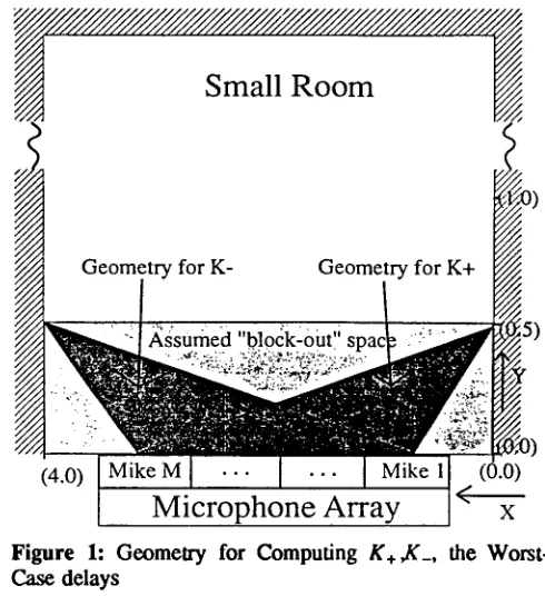
the geometry shown

in Figure 1 for a onedimensional array. For a symmetric

arrangement in a room. K- =

K +

and

R

K- = K+ = r k n g t h -cos(O)-1.

C (2.7)

where c is the speed of sound with value about 342M/s.

Small Room

Geometry for K+

[image:2.612.318.563.366.634.2]

I

Figure 1: Geometry for Computing K+&-, the Worst-

Case delays

(4.0)

As an example, consider a one-dimensional array of

length one meter, a room four meters wide, one-half me-

ter of "block-out space" and a sampling rate of 20,000 samples-per-second. For this case, correlations will re- quire 2000 multiplication-addition operations for lOOmsec of data. As the maximum relative delay may be seen to

be 1'C0S140 = 2.84m.s. Equation (2.7) yields

C

K- = K+ = 57. Thus, the correlation phase requires

Mike M

I

. . .

I

. . .

I

Mike 1

Microphone

Array

(0.0)

L

(3)

L R"

B= (k ")

= OR OR

230,000 multiplication-additions per microphone pair if done directly or just under 20ms of computation time using the Analog Devices ADSP-2100A digital signal pro- cessor at 12.5MHz clock rate [16]. For eight microphones, about 160 ms would be required, and the location could be computed in real-dine for the required five up- dates per second.

The relative delay between each microphone and its reference could be estimated by selecting the highest positive point in the correlation outputs, i.e.,

k=* -= argmin C~[k,k'], (2.8) -.K_ ~l ~K+

k:, (2.9)

d, tk q

-

"T'

where d,~ [k'] is defined to be the delay, relative to microphone 1, for microphone m. Note that the accuracy is only to that of the sample rate, and that this simple peak- picking algorithm is subject to serious errors when real data are used!

Interpolation for Higher Accuracy

Even for the relatively high (for speech) sampling rate of 20kHz, estimation accuracy of the tracking position is inadequate; a variation of more than one meter in the y dimension is the norm for talkers two meters directly in front of the microphone. Experience has shown that an acceptable region of uncertainty may be achieved for a sampling inteerval of about llas.

The most straightforward way to achieve the needed high resolution would be to sample at a much higher rate, R" -- around 1MHz - and perform the correlations on the data, i.e.,

C,~'[k,kq= B.(k3 LR'-~

_{E r~'(k'+l).r~'(k'+k+l)(3.1)}

LtC--lk l I=o

where B , ( k ' ) is a normalizing factor and L R' is the number of high-resolution samples in L. Relative to 20kHz sampling, this would force the computation to increase by a factor of 502 = 2500, making the procedure absurd. For an appropriately anti-aliased speech signal, one would be dealing with greatly oversampled signals. Thus, with no loss in accuracy, one could generate the signal at sampling rate R ' from the signal sampled at rate R by the simplest standard multirate method if

R" -= Z'R, (3.2)

where 2~ is an integer greater than 1.

The proof for computationally efficient interpolation is given in [17]. The results for computation are:

B m (k ') QR QR

=

~

E (3.3)

C~'[~offk+Vt, k'] L l ' - I~Jfftt +Vk I at=._QR~2=._QR

• [a,, a2. vk ]-C,~ [k + a~-a2 ,kq

~ ~[~i, OZ 0]'CUR [ ~ t - O2 ,k'~ 3"4) at= ..QRa2= ..QR

"7

}

• [al,a2vi] n ~

(7~l+vi)'f(~2+vk+vl)

(3.5)

Vl= 0

C,~ [ k "t.ff l--o2 k "] m L-Ik-c-qfft--ff21

A . ( k 3 (3.6)

C~[k+Gl-Cr 2, k•

Computational Considerations for the Inter-

polation

One important aspect of the computation of Equa- tion (3.3) is the storage requirement for O. Appropriate resolution is achieved for Z=64, R=20k.Hz and a filter length of 641, implying QR =5. Then the range of oi and 02 is only 11. Thus (11)(11)(64) = 7744 storage locations are required.

The number of multiplication-additions is (11)2= 121 to compute the cross-correlation for each interpolated point. One should note that this number is a far cry from the "direct" method in which, for L = 2000, (621)(64)(2000) = 80,000,000 operations had to be done to get each interpolated signal and (64)(2000) = 128,000 operations had to be done for each interpolated cross- correlation!

Best Hyperbolic Fit Algorithms

Triangulation

In binaural hearing, both amplitude and phase infor- marion is fed to the ~ and is used -- expertly -- to determine the location of a sound source. If the phase information -- the delay estimates - alone were to be used to determine location of a source, a minimum of three microphones is required for this "triangulation" procedure. If microphone 1 is considered to be the reference, and d2 and d3 the time delays for microphones 2 and 3 respec- tively, relative to the arrival at microphone 1, then the estimation of the source location xo, Yo may be determined from,

¢ 2d 22 (d2 - d 3)-d 2(z 32-z 12 ) + d 3(z 22-z 12 ) x0 = 2[d2(z 1 -z 3) - d3(z 1-z 2)] (4.1)

12

YO = t~

~

j

-(Xo-Zl)2J . ( 4 . 2 )

(One should note that these triangulation formulae are normally listed for polar coordinates.) These relatively ugly, nonlinear expressions tend to be very sensitive to variations due to noise in the estimates of d2 and d3.

(4)

T i m e - D e l a y E s t i m a t i o n , H y p e r b o l i c Fit

( T D E H F )

For the case of the linear array, where the microphones are all considered to be on y=0, the locus of the relative delays for points along this line forms a hyperbola. This is clear from Figure 2 in which the relative delay loci are plotted for various point-source locations (x,y). At (zm,0), the absolute delay d= may be computed from the Pythagorean Theorem as

d m - " ~ ] ( X - z 2 ) + y 2 (4.3)

C ,

and, relative to microphone 1,

d,~ = ~l(x-zm)2+y2

dr.

(4.4)

C

Some algebra yields,

(d,~+dl) 2 -

(Zm-X)2

= ~ (4.5) C 2 C 2 "

The points ( z = , d . ) lie on a hyperbola parameterized by the speed of sound, c, and the location of the source, ( x , y ) . Thus, there is a one-to-one relationship between a specific hyperbola and a source-point

(x,y)

located in front of the array -- there is a mirror in back of the array. The task, then, is to fit the best member of this class, the best hyperbola, to the set of relative delay estimates

zmd,~'[l~'],

where m e [2,M]. "~ it. ~-

E

o-i

u 1

t_ [D CO

0.5

C

o

ua 1:3 .,..4

t_ -6.5

q3

E C3 t_ -1

> . r13

oJ -1.5

~ l0 28 30 48 50 60 70 80 90 (0.44m,0.0.) / Nicroohone Placement (cm)

Figure 2: Delay Hyperbolae for Several Source Locations In TDEHF an estimate of the relative delay for each microphone is obtained by peak-picking as indicated by Equations (2.10) and (2.11). Interpolation is done lo- cally to get a higher resolution estimate,

d,~'(k').

While many criteria are possible, a typical squared-error measure is defined as

M

E (k') = 2~ (d,~ "(k 3 - d,,))2

(4.6)

m=2

Substituting (4.4) into (4.6), one gets,

Source Location

" - - - 7

-o- 10.25m, l . ~ m )

"-+- (0.65ml 1.Sin) ]

-o-(l.8m,2.0m) [

-~-" (1.35m, 1.5m) I

M[ d

. ~ ( X _ Z m ) 2 + y 2 ] 2

E(k 3 = E

,~'(k')

- d t

(4.7)

m=2 C

and the esrtimate (x0,yd minimizes

E(k'). As

this surface is normally unimodal, a gradient method [18] has been used.

I n t e r p o l a t e d C r o s s - c o r r e l a t i o n H y p e r b o l i c Fit

( I C H F )

When real data are used, it is often the case that the cross-correlation peak which must be determined in

TDEHF is inappropriate. This is due to 1) periodicity in the signal, 2) room reverberations, and 3) noise. A more robust algorithm would clearly resdt ff the specific deter- mination of the delays did not have to be explicitly done. In ICHF, one tries to determine the "optimal:fit" hyperbola in the cross.correlation space itself; thus, no pattern recognition errors are made prior to the optimization.

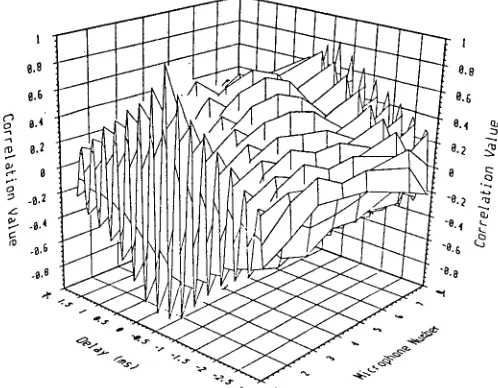
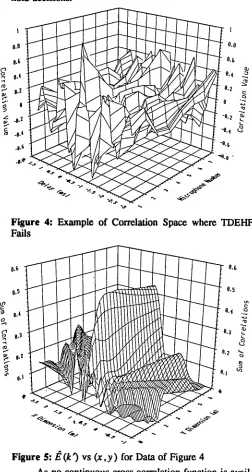
Plots for real data are presented in Figures 3 and 4. In each case, the d at~ are produced by a loud talker si- tuated at (1M,2M) with low ambient noise. In Figure 3, TDEHF worked well, as the peaks are relatively easy to pick correctly. In Figure 4, however, TDEHF yielded poor results, although it is evident that a hyperbolic fit in the cross-correlation space itself could give the right location.

6.8 8.8

8.6

~ o.2

.~,2

Figure 3: Example of Correlation Space where TDEHF Succeeds

In nonlinear optimization, one must develop a functional that measures "goodness (badness)" as a function of the set of variables over which one wants to optimize. In this case, one wants to develop a measure of the average "goodness" of a particular hyperbola parametefized by ( x , y ) over the space shown in Figures 3, 4 having independent variables of x , the x spatial variable, and i f , the relative delay. Points for the microphones

(z,,,,d,,)

[image:4.612.319.568.366.560.2]

(5)

M

I .

--- . - ,

/~(k') represents a measure of the average height of the cross-correlation function measured over the points on the hyperbola taken by the set of microphones. One should note that it would be expected that the value should be positive for reasonable situations, and approaching unity for ideal ones, and thus/~ (k') could also be used to thres- hold decisions.

@.8 8.8

8.6 8.6

~.~ ~.e •

Figure 4: Example of Correlation Space where TDEI-IF Fails

@.6

~

8.~

° H4 k qgggE'H i

@.3

8'3

[image:5.612.53.305.155.627.2] [image:5.612.56.301.164.367.2] [image:5.612.331.562.387.569.2]

,.' t I _ ~ # L t ~ I ~ / I I U J _ . L , H ] ~ I J , I I . , ~ I ! " °

Figure 5:/~(k3 vs (x,y) for Data of Figure 4

As no continuous cross-correlation function is avail- able, one must approximate it. It is assumed that interpolation may be used to achieve an accurate estimate, i. e., one determines Om and v . from d,~ using,

* ,LJ _>o

=- M * , L - L o J ,L <0" (4.9)

v . .

ta.,R'- o . * + 0.sj.

Then, C . ( z . . din) may be accurately approximated by

Cm(zm.dm)

= C~'[~m +vm,k'], (4.11)

which is exactly as derived previously. A three dimensional plot of the surface for E (k 3 is given in Figure 5. Notice the strong peaking due to the hyperbolic-fit transformation.

R e s u l t s

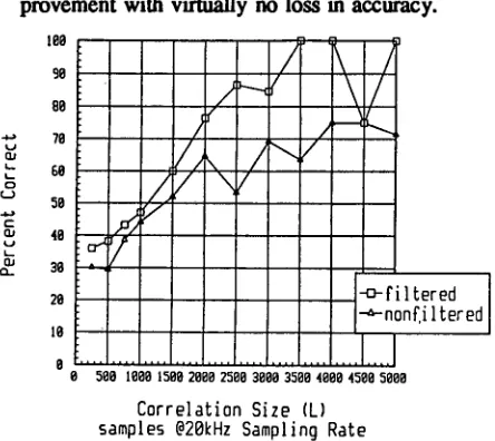
Some preliminary results for one loud talker stand- ing at (1M,2M) with a low ambient are shown in Figures 6 and 7. A linear array of eight microphones was used for all cases. For these Figures, an algorithm was assumed to have c(rrecfly located the talker ff it indicated a location within the rectangular region from 1.9M to 2.1M in x and 1.5M to 2.5M in y. As algorithms have improved, the measure of "correctness" is also to be refined in further work. In both TDEHF and ICHF, the tendency is for better p e r f o r m a n c e when larger-size crosscorrelations are used, although there seems to be no rea- son to go beyond 3500 samples (175ms). It is also clear that ICHF is far more robust than is TDEHF. Further- more, as might be expected, one gets improved performance using bandpass-filtered data. (The filter used is a 61-tap, symmetric FIR filter having transition bands (400Hz -900Hz) and (3300HZ-3800)Hz; stopbands are 50dB down.)

u t _ o

5@

c

48

m 3@

I@@

I"

9@

- o - f i ] feted

88 -~-n0n f i ] t e r e d

78

/ [ \ %6"I I I \

Correlation Size (L) samples @2@kHz Sampling Rate

Figure 6: Performance of TDEHF

There is high correlation between "correctness" and the resultant value of/~ [k q for ICHF. Therefore, it is expected that, in regions where the algorithm fails -- perhaps in silence or a high-ambient interval -- the value of

E[k']

would be low and the incorrect location would not be accepted. Given this thresholding, one would ex- pect to almost always get an accurate prediction of a talker's location, providing no other talkers are competing acoustically, a case not yet studied.

Computationally, ICHF is implementable in real- time due to the use of Stochastic Region Contraction [14] for the nonlinear optimization. Relative to a coarse-fine full search, SRC has provided an order-of-magnitude im-

(6)

pmvement with virtl,aUy no loss in accuracy.

Q~

0_ 188

g8

88

78

5 8

58

48

38

28

16

8

/

\ /

• i i

!

,-°-filtered ]

J-~-

non

Ci

I

tered

. . . ... I ....

I

8 500 I~08 158~ 2 8 0 8 2500 3888 3588 4 8 8 8 4588 5888

Correlation

Size (L)

samples @20kHz Sampling

Rate

Figure 7: Performance of ICHF

Conclusion

A very promising algorithm for determining the location of a talker in a real acoustic environment has been introduced. In an uncontested acoustic environment, preliminary results from real data indicate that highly accurate performance is achievable. In addition, the SRC method for nonlinear optimization has provided a mechanism for making the algorithm practical in real time. In follow-on work, more data have to be tested, multiple talker and various noise environments need to be explored, and extensions to tracking need to be developed. However, the current level of performance tends to predict that these aspects will go smoothly.

References

[1] Flanagan, J. L., Bandwidth Design for Speech-seeking Microphone Arrays, Proc. 1985 ICASSP, Tampa, FL, 3/85, pp. 732-735.

[2] Martin, T. B., Practical Applications of Voice Input to Machines, Proceedings IEEE, Vol. 64, 4/'76 pp. 487-501.

[3] Flanagan, J. L., Johnston, J. D., Zahn, R., and Elko,

G. W., Computer-steered Microphone Arrays for Source Transduction fll Large Rooms, Journal of the Acoustical Society of America, Vol. 78, No. 5, 11/85, pp. 1508- 1518.

[4] Schmidt, R. 0., A Signal Subspace Approach to Multi- ple Emitter Location and Spectral Estimation, PhD.

Dissertation, Stanford University, Nov. 1981.

[5] Schmidt, R. O., Multiple Emitter Location and Signal Parameter Estimation, IEEE Trans. on Antennas and Pro- pagation, Vol. AP-34, No. 3, 3/86, pp. 276-280.

[6] Schmidt, R. O., and Franks, R. E., Multiple Source DF Signal Processing: An Experimental System, IEEE Trans. on Antennas and Propagation, Vol. AP-34, No. 3, 3/86, pp. 281-290.

[7] Wax, M. and Kailath, T., Optimum Localization of

Multiple Sources by Passive Arrays, IEEE Trans. on Acoustics, Speech and Signal Processing, Vol. ASSP-31, No. 5, 10/83, pp. 1210-1218.

[8] Kesler, S. B., and Shahmirian, V., Bias Resolution of the MUSIC and Modified FBLP Algorithms in the Pres- ence of Coherent Plane Waves, IEEE Trans. on Acous- tics, Speech and signal Processing, Vol ASSP-36, No. 8, 8/88, pp. 1351-1352.

[9] Knapp, C. H., and Carter, G. C., The Generalized Correlation Method for Estimation of Time delay, IEEE

Transactions on Acoustics, Speech and Signal Processing, Vol. ASSP-24, No. 4, 8/76, pp. 320-327.

[10] Carter, G. C., Coherence and Time-Delay Estimation,

Proc. IEEE, Vol. 75, No. 2, 2/87, pp. 236-255.

[11] Bendat, J. S., and Piersol, A. G., Engineering Appli- cations of Correlation and Spectral Analysis, John Wiley and Sons, Inc. 1980.

[12] Crochiere, R. E., and Rabiner, L. R., Multirate Digi- tal Signal Processing, Prentice-Hall, Englewood Cliffs, NJ 07632, 1983.

[13] Press, W. H., Flannery, B. P., Teukolsky, S. A., and Vettering, W. T., Numerical Recipes in C, Cambridge University Press, New York, 1988.

[14] Bergex, M., and Silverman, H. F., Microphone Array Optimization by Stochastic Region Contraction, Technical Report LEMS-62, Division of Engineering, Brown University, August 1989.

[15] Alvarado, V. M., Talker Localization and Optimal Placement of Microphones for a Linear Microphone Ar- ray using StochasticRegion Contraction, PhD Thesis, LEMS, Division of Engineering, Brown University, May

1990.

[16] Analog Devices, Inc. ADSP-2100 User's Manual,

Analog Devices, Inc., Norwood, MA, 1989.

[17] Silverman, H. F., and Doerr, K. J., Talker Location using a Linear Microphone Array and Hyperbolic Fitting

Brown University, Division of Engineering, LEMS Technical Report #73, July 1990.

[image:6.612.54.276.50.248.2]