Random Fields: Parameterised Versus
Parameter-Free
Andrew Smith and Miles Osborne
School of Informatics, University of Edinburgh, United Kingdom
[email protected], [email protected]
Abstract. Recent work on Conditional Random Fields (CRFs) has demonstrated the need for regularisation when applying these models to real-world NLP data sets. Conventional approaches to regularising CRFs has focused on using a Gaussian prior over the model parameters. In this paper we explore other possibilities for CRF regularisation. We examine alternative choices of prior distribution and we relax the usual simplifying assumptions made with the use of a prior, such as constant hyperparameter values across features. In addition, we contrast the effec-tiveness of priors with an alternative, parameter-free approach. Specifi-cally, we employlogarithmic opinion pools(LOPs). Our results show that a LOP of CRFs can outperform a standard unregularised CRF and attain a performance level close to that of a regularised CRF, without the need for intensive hyperparameter search.
1
Introduction
Recent work on Conditional Random Fields (CRFs) has demonstrated the need for regularisation when applying these models to real-world NLP data sets ([8], [9]). Standard approaches to regularising CRFs, and log-linear models in general, has focused on the use of a Gaussian prior. Typically, for simplicity, this prior is assumed to have zero mean and constant variance across model parameters. To date, there has been little work exploring other possibilities. One exception is Peng & McCallum [8]. They investigated feature-dependent variance for a Gaus-sian prior, and explored different families of feature sets. They also compared different priors for CRFs on an information extraction task.
In the first part of this paper, we compare priors for CRFs on standard sequence labelling tasks in NLP: NER and POS tagging. Peng & McCallum used variable hyperparameter values only for a Gaussian prior, based on feature counts in the training data. We use an alternative Bayesian approach to mea-sure confidence in empirical expected feature counts, and apply this to all the priors we test. We also look at varying the Gaussian prior mean. Our results show that: (1) considerable search is required to identify good hyperparameter values for all priors (2) for optimal hyperparameter values, the priors we tested perform roughly equally well (3) in some cases performance can be improved using feature-dependent hyperparameter values.
R. Dale et al. (Eds.): IJCNLP 2005, LNAI 3651, pp. 896–907, 2005. c
As can be seen, a significant short-coming of using priors for CRF regular-isation is the requirement for intensive search of hyperparameter space. In the second part of the paper we contrast this parameterised prior approach with an alternative, parameter-free method. We factor the CRF distribution into a weighted product of individual expert CRF distributions, each focusing on a particular subset of the distribution. We call this model alogarithmic opinion pool(LOP) of CRFs (LOP-CRFs).
Our results show that LOP-CRFs, which are unregularised, can outperform the unregularised standard CRF and attain a performance level that rivals that of the standard CRF regularised with a prior. This performance may be achieved with a considerably lower time for training by avoiding the need for intensive hyperparameter search.
2
Conditional Random Fields
A linear chain CRF defines the conditional probability of a label sequence s given an observed sequenceovia:
p(s|o) = 1
whereTis the length of both sequences,λkare parameters of the model andZ(o) is the partition function that ensures (1) represents a probability distribution. The functions fk are feature functions representing the occurrence of different events in the sequencessando.
The parameters λk can be estimated by maximising the conditional log-likelihood of a set of labelled training sequences. The log-log-likelihood is given by:
LL(λ) =
where ˜p(s|O) and ˜p(o) are empirical distributions defined by the training set. At the maximum likelihood solution the model satisfies a set of feature constraints, whereby the expected count of each feature under the model is equal to its empirical count on the training data:
Ep(˜o,s)[fk]−Ep(s|o)[fk] = 0, ∀k
In general this cannot be solved for theλk in closed form so numerical routines
must be used. Malouf [6] and Sha & Pereira [9] show that gradient-based algo-rithms, particularly limited memory variable metric (LMVM), require much less time to reach convergence, for some NLP tasks, than the iterative scaling meth-ods previously used for log-linear optimisation problems. In all our experiments we use the LMVM method to train the CRFs.
For CRFs with general graphical structure, calculation of Ep(s|o)[fk] is
dynamic programming procedure for inference, similar in nature to the forward-backward algorithm in hidden Markov models.
Given a trained CRF model defined as in (1), the most probable labelling under the model for a new observed sequenceois given by argmaxsp(s|o). This can be recovered efficiently using the Viterbi algorithm.
3
Parameterised Regularisation: Priors for CRFs
Most approaches to CRF regularisation have focused on the use of a prior distri-bution over the model parameters. A prior distridistri-bution encodes prior knowledge about the nature of different models. However, prior knowledge can be difficult to encode reliably and the optimal choice of prior family may vary from task to task. In this paper we investigate the use of three prior families for the CRF.
3.1 Gaussian Prior
The most common prior used for CRF regularisation has been the Gaussian. Use of the Gaussian prior assumes that each model parameter is drawn independently from a Gaussian distribution. Ignoring terms that do not affect the parameters, the regularised log-likelihood with a Gaussian prior becomes:
LL(λ)−1 2
k
λk−µk σk
2
where µk is the mean and σk the variance for parameter λk. At the optimal point, for eachλk, the model satisfies:
E˜p(o,s)[fk]−Ep(s|o)[fk] =
λk−µk σ2
k
(2)
Usually, for simplicity, eachµk is assumed zero and σk is held constant across
the parameters. In this paper we investigate other possibilities. In particular, we allow the means to take on non-zero values, and the variances to be feature-dependent. This is described in more detail later. In each case values for means and variances may be optimised on a development set.
We can see from (2) that use of a Gaussian prior enforces the constraint that the expected count of a feature under the model is discounted with respect to the count of that feature on the training data. As discussed in [1], this corresponds to a form of logarithmic discounting in feature count space and is similar in nature to discounting schemes employed in language modelling.
3.2 Laplacian Prior
Use of the Laplacian prior assumes that each model parameter is drawn inde-pendently from the Laplacian distribution. Ignoring terms that do not affect the parameters, the regularised log-likelihood with a Laplacian prior becomes:
LL(λ)−
k
whereβk is a hyperparameter, and at the optimal point the model satisfies:
Ep(˜o,s)[fk]−Ep(s|o)[fk] =
sign(λk)
βk , λk = 0 (3)
Peng & McCallum [8] note that the exponential prior (a one-sided version of the Laplacian prior here) represents applying an absolute discount to the empirical feature count. They fix theβk across features and set it using an expression for the discount used in absolute discounting for language modelling. By contrast we allow theβk to vary with feature and optimise values using a development set.
The derivative of the penalty term above with respect to a parameterλk is
discontinuous atλk = 0. To tackle this problem we use an approach described
by Williams, who shows how the discontinuity may be handled algorithmically [13]. His method leads to sparse solutions, where, at convergence, a substantial proportion of the model parameters are zero. The result of this pruning effect is different, however, to feature induction, where features are included in the model based on their effect on log-likelihood.
3.3 Hyperbolic Prior
Use of the hyperbolic prior assumes that each model parameter is drawn inde-pendently from the hyperbolic distribution. Ignoring constant terms that do not involve the parameters, the regularised log-likelihood becomes:
LL(λ)−
k
log
eβkλk+ e−βkλk
2
whereβk is a hyperparameter, and at the optimal point the model satisfies:
Ep(˜o,s)[fk]−Ep(s|o)[fk] =βk
eβkλk−e−βkλk
eβkλk+ e−βkλk
(4)
3.4 Feature-Dependent Regularisation
For simplicity it is usual when using a prior to assume constant hyperparameter values across all features. However, as a hyperparameter value determines the amount of regularisation applied to a feature, we may not want to assume equal values. We may have seen some features more frequently than others and so be more confident that their empirical expected counts are closer to the true expected counts in the underlying distribution.
Peng & McCallum [8] explore feature-dependent variance for the Gaussian prior. They use different schemes to determine the variance for a feature based on its observed count in the training data. In this paper we take an alternative, Bayesian approach motivated more directly by our confidence in the reliability of a feature’s empirical expected count.
data. It is natural, therefore, that the size of this discount, controlled through a hyperparameter, is related to our confidence in the reliability of the empiri-cal expected count. We formulate a measure of this confidence. We follow the approach of Kazama & Tsujii [4], extending it to CRFs.
The empirical expected count,Ep(˜o,s)[fk], of a featurefk is given by:
Now, our CRF features have the following form:
fk(st−1, st,o, t) =
1 if st−1=s1,st=s2 andhk(o, t) = 1
0 otherwise
wheres1ands2are the labels associated with featurefkandhk(o, t) is a binary-valued predicate defined on observation sequence o at position t. With this feature definition, and contracting notation for the empirical probability to save space,Ep(˜o,s)[fk] becomes:
Contributions to the inner sum are only made at positionstin sequenceowhere thehk(o, t) = 1. Suppose that we make the assumption that at these positions
˜
Now, if we assume that we can get a reasonable estimate of ˜p(o) from the training data then the only source of uncertainty in the expression forEp(˜o,s)[fk] is the term
˜
p(st−1=s1, st=s2|hk(o, t) = 1). Assuming this term is independent of sequence
oand positiont, we can model it as the parameterθof a Bernoulli random variable that takes the value 1 when featurefkis active and 0 when the feature is not active buthk(o, t) = 1. Suppose there areaandbinstances of these two events, respec-tively. We endow the Bernoulli parameter with a uniform prior Beta distribution Be(1,1) and, having observed the training data, we calculate the variance of the posterior distribution, Be(1 +a, 1 +b). The variance is given by:
We use this variance as a measure of the confidence we have inEp(˜o,s)[fk] as an
estimate of the true expected count of feature fk. We therefore adjust hyper-parameters in the different priors according to this confidence for each feature. Note that this value for each feature can be calculated off-line.
4
Parameter-Free Regularisation: Logarithmic Opinion
Pools
So far we have considered CRF regularisation through the use of a prior. As we have seen, most prior distributions are parameterised by a hyperparameter, which may be used to tune the level of regularisation. In this paper we also consider a parameter-free method. Specifically, we explore the use of logarithmic opinion pools [3].
Given a set of CRF model experts with conditional distributions pα(s|o) and a set of non-negative weightswαwithαwα= 1, alogarithmic opinion poolis defined as the distribution:
¯
p(s|o) = ¯1
Z(o)
α
[pα(s|o)]wα, with ¯Z(o) = s
α
[pα(s|o)]wα
Suppose that there is a “true” conditional distribution q(s|o) which each
pα(s|o) is attempting to model. In [3] Heskes shows that the KL divergence betweenq(s|o) and the LOP can be decomposed as follows:
K(q,p¯) =
α
wαK(q, pα)−
α
wαK(¯p, pα) =E−A (5)
This explicitly tells us that the closeness of the LOP model toq(s|o) is governed by a trade-off between two terms: anE term, which represents the closeness of the individual experts toq(s|o), and anAterm, which represents the closeness of the individual experts to the LOP, and therefore indirectly to each other. Hence for the LOP to modelq well, we desire modelspα which are individually good models ofq (having lowE) and are also diverse (having largeA).
Training LOPs for CRFs. The weightswαmay be defined a priori or may be
found by optimising an objective criterion. In this paper we combine pre-trained expert CRF models under a LOP and train the weights wα to maximise the
likelihood of the training data under the LOP. See [10] for details.
5
The Tasks
In this paper we compare parametric and LOP-based regularisation techniques for CRFs on two sequence labelling tasks in NLP:named entity recognition (NER) andpart-of-speech tagging(POS tagging).
5.1 Named Entity Recognition
All our results for NER are reported on the CoNLL-2003 shared task dataset [12]. For this dataset the entity types are: persons (PER), locations (LOC), organisations (ORG) and miscellaneous (MISC). The training set consists of 14,987 sentences and 204,567 tokens, the development set consists of 3,466 sentences and 51,578 tokens and the test set consists of 3,684 sentences and 46,666 tokens.
5.2 Part-of-Speech Tagging
For our experiments we use the CoNLL-2000 shared task dataset [11]. This has 48 different POS tags. In order to make training time manageable, we collapse the number of POS tags from 48 to 5 following the procedure used in [7]. In summary: (1) All types of noun collapse to category N. (2) All types of verb collapse to category V. (3) All types of adjective collapse to category J. (4) All types of adverb collapse to category R. (5) All other POS tags collapse to categoryO. The training set consists of 7,300 sentences and 173,542 tokens, the development set consists of 1,636 sentences and 38,185 tokens and the test set consists of 2,012 sentences and 47,377 tokens.
5.3 Experts and Expert Sets
As we have seen, our parameter-free LOP models require us to define and train a number of expert models. For each task we define a single, complex CRF, which we call amonolithicCRF, and a range of expert sets. The monolithic CRF for NER comprises a number of word and POS features in a window of five words around the current word, along with a set of orthographic features defined on the current word. The monolithic CRF for NER has 450,345 features. The monolithic CRF for POS tagging comprises word and POS features similar to those in the NER monolithic model, but over a smaller number of orthographic features. The monolithic model for POS tagging has 188,488 features.
Each of our expert sets consists of a number of CRF experts. Usually these experts are designed to focus on modelling a particular aspect or subset of the distribution. The experts from a particular expert set are combined under a LOP-CRF with the unregularised monolithic CRF.
monolithic model. The reduced model comprises 24,818 features for NER and 47,420 features for POS tagging. (2)Positionalconsists of the monolithic CRF and a partition of the features in the monolithic CRF into three experts, each consisting only of features that involve events either behind, at or ahead of the current sequence position. (3)Labelconsists of the monolithic CRF and a partition of the features in the monolithic CRF into five experts, one for each label. For NER an expert corresponding to label X consists only of features that involve labels B-X or I-X at the current or previous positions, while for POS tagging an expert corresponding to label X consists only of features that involve label X at the current or previous positions. These experts therefore focus on trying to model the distribution of a particular label. (4)Random consists of the monolithic CRF and a random partition of the features in the monolithic CRF into four experts. This acts as a baseline to ascertain the performance that can be expected from an expert set that is not defined via any linguistic intuition.
6
Experimental Results
For each task our baseline model is the monolithicmodel, as defined earlier. All the smoothing approaches that we investigate are applied to this model. For NER we report F-scores on the development and test sets, while for POS tagging we report accuracies on the development and test sets.
6.1 Priors
Feature-Independent Hyperparameters. Tables 1 and 2 give results on the two tasks for different priors with feature-independent hyperparameters. In the case of the Gaussian prior, the mean was fixed at zero with the variance being the adjustable hyperparameter. In each case hyperparameter values were optimised on the development set. In order to obtain the results shown, extensive search of the hyperparameter space was required. The results show that: (1) For each prior there is a performance improvement over the unregularised model. (2) Each of the priors gives roughly the same optimal performance.
These results are contrary to the conclusions of Peng & McCallum in [8]. On an information extraction task they found that the Gaussian prior performed
Table 1.F-scores for priors on NER
Prior Development Test
Unreg. monolithic 88.33 81.87
Gaussian 89.84 83.98
Laplacian 89.56 83.43
Hyperbolic 89.84 83.90
Table 2.Accuracies for priors on POS tagging
Prior Development Test
Unreg. monolithic 97.92 97.65
Gaussian 98.02 97.84
Laplacian 98.05 97.78
significantly better than alternative priors. Indeed they appeared to report per-formance figures for the hyperbolic and Laplacian priors that were lower than those of the unregularised model. There are several possible reasons for these differences. Firstly, for the hyperbolic prior, Peng & McCallum appeared not to use an adjustable hyperparameter. In that case the discount applied to each empirical expected feature count was dependent only on the current value of the respective model parameter and corresponds in our case to using a fixed value of 1 for theβ hyperparameter. Our results for this value of the hyperparameter are similarly poor. The second reason is that for the Laplacian prior, they again used a fixed value for the hyperparameter, calculated via an absolute discount-ing method used language modelldiscount-ing [1]. Havdiscount-ing achieved poor results with this value they experimented with other values but obtained even worse performance. By contrast, we find that, with some search of the hyperparameter space, we can achieve performance close to that of the other two priors.
Feature-Dependent Hyperparameters. Tables 3 and 4 give results for dif-ferent priors with feature-dependent hyperparameters. Again, for the Gaussian prior the mean was held at 0. We see here that trends differ between the two tasks. For POS tagging we see performance improvements with all the priors over the corresponding feature-independent hyperparameter case. Using McNemar’s matched-pairs test [2] on point-wise labelling errors, and testing at a significance level of 5% level, all values in Table 4 represent a significant improvement over the corresponding model with feature-independent hyperparameter values, ex-cept the one marked with∗. However, for NER the opposite is true. There is a performance degradation over the corresponding feature-independent hyperpa-rameter case. Values marked with† are significantly worse at the 5% level. The hyperbolic prior performs particularly badly, giving no improvement over the unregularisedmonolithic. The reasons for these results are not clear. One pos-sibility is that defining the degree of regularisation on a feature specific basis is too dependent on the sporadic properties of the training data. A better idea may be to use an approach part-way between feature-independent hyperparameters and feature-specific hyperparameters. For example, features could be clustered based on confidence in their empirical expected counts, with a single confidence being associated with each cluster.
Varying the Gaussian Mean. When using a Gaussian prior it is usual to fix the mean at zero because there is usually no prior information to suggest penal-ising large positive values of model parameters any more or less than large
mag-Table 3.F-scores for priors on NER
Prior Development Test
Gaussian 89.43 83.27† Laplacian 89.28 83.37
Hyperbolic 88.34† 81.63†
Table 4.Accuracies for priors on POS tagging
Prior Development Test
Gaussian 98.12 97.88∗ Laplacian 98.12 97.92
nitude negative values. It also simplifies the hyperparameter search, requiring the need to optimise only the variance hyperparameter. However, it is unlikely that optimal performance is always achieved for a mean value of zero.
To investigate this we fix the Gaussian variance at the optimal value found earlier on the development set, with a mean of zero, and allow the mean to vary away from zero. For both tasks we found that we could achieve significant performance improvements for non-zero mean values. On NER a model with mean 0.7 (and variance 40) achieved an F-score of 90.56% on the development set and 84.71% on the test set, a significant improvement over the best model with mean 0. We observe a similar pattern for POS tagging. These results suggest that considerable benefit may be gained from a well structured search of the joint mean and variance hyperparameter space when using a Gaussian prior for regularisation. There is of course a trade-off here, however, between finding better hyperparameters values and suffering increased search complexity.
6.2 LOP-CRFs
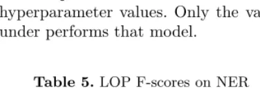
Tables 5 and 6 show the performance of LOP-CRFs for the NER and POS tagging experts respectively. The results demonstrate that: (1) In every case the LOPs significantly outperform the unregularisedmonolithic. (2) In most cases the performance of LOPs is comparable to that obtained using the different priors on each task. In fact, values marked with‡show a significant improvement over the performance obtained with the Gaussian prior with feature-independent hyperparameter values. Only the value marked with † in Table 6 significantly under performs that model.
Table 5.LOP F-scores on NER
Expert set Development set Test set
Unreg. monolithic 88.33 81.87
Simple 90.26 84.22‡
Positional 90.35 84.71‡
Label 89.30 83.27
Random 88.84 83.06
Table 6.LOP accuracies on POS tagging
Expert set Development set Test set
Unreg. monolithic 97.92 97.65
Simple 98.31‡ 98.12‡ Positional 98.03 97.81
Label 97.99 97.77
Random 97.99 97.76†
do not focus on any one aspect or subset of it. Intuitively, then, we want to devise experts that are simultaneously diverse and accurate.
The advantage of the LOP-CRF approach over the use of a prior is that it is “parameter-free” in the sense that each expert in the LOP-CRF is unregu-larised. Consequently, we are not required to search a hyperparameter space. For example, to carefully tune the hyperbolic hyperparameter in order to obtain the optimal value we report here, we ran models for 20 different hyperparameter values. In addition, in most cases the expert CRFs comprising the expert sets are small, compact models that train more quickly than themonolithicwith a prior, and can be trained in parallel.
7
Conclusion
In this paper we compare parameterised and parameter-free approaches to smoothing CRFs on two standard sequence labelling tasks in NLP. For the parameterised methods, we compare different priors. We use both feature-independent and feature-dependent hyperparameters in the prior distributions. In the latter case we derive hyperparameter values using a Bayesian approach to measuring our confidence in empirical expected feature counts. We find that: (1) considerable search is required to identify good hyperparameter values for all priors (2) for optimal hyperparameter values, the priors we tested perform roughly equally well (3) in some cases performance can be improved using feature-dependent hyperparameter values.
We contrast the use of priors to an alternative, parameter-free method using logarithmic opinion pools. Our results show that a LOP of CRFs, which contains unregularised models, can outperform the unregularised standard CRF and at-tain a performance level that rivals that of the standard CRF regularised with a prior. The important point, however, is that this performance may be achieved with a considerably lower time for training by avoiding the need for intensive hyperparameter search.
References
1. Chen, S. and Rosenfeld, R.: A Survey of Smoothing Techniques for ME Models. IEEE Transactions on Speech and Audio Processing (2000) 8(1) 37–50
2. Gillick, L., Cox, S.: Some statistical issues in the comparison of speech recognition algorithms. ICASSP (1989) 1 532–535
3. Heskes, T.: Selecting weighting factors in logarithmic opinion pools. NIPS (1998) 4. Kazama, J. and Tsujii, J.: Evaluation and Extension of Maximum Entropy Models
with Inequality Constraints. EMNLP (2003)
5. Lafferty, J. and McCallum, A. and Pereira, F.: Conditional Random Fields: Prob-abilistic Models for Segmenting and Labeling Sequence Data. ICML (2001) 6. Malouf, R.: A comparison of algorithms for maximum entropy parameter
estima-tion. CoNLL (2002)
8. Peng, F. and McCallum, A.: Accurate Information Extraction from Research Pa-pers using Conditional Random Fields. HLT-NAACL (2004)
9. Sha, F. and Pereira, F.: Shallow Parsing with Conditional Random Fields. HLT-NAACL (2003)
10. Smith, A., Cohn, T., Osborne, M.: Logarithmic Opinion Pools for Conditional Random Fields. ACL (2005)
11. Tjong Kim Sang, E. F. and Buchholz, S.: Introduction to the CoNLL-2000 shared task: Chunking. CoNLL (2000)
12. Tjong Kim Sang, E. F. and De Meulder, F.: Introduction to the CoNLL-2003 Shared Task: Language-Independent Named Entity Recognition. CoNLL (2003) 13. Williams, P.: Bayesian Regularisation and Pruning using a Laplace Prior. Neural