Optimisation of Area Traffic Control for Equilibrium Network Flows

(1)

Optimisation of Area Traffic Control for Equilibrium Network Flows

Suh-Wen Chiou

A thesis submitted to the University of London for the Degree of Doctor of Philosophy

Centre for Transport Studies

(2)

ProQuest Number: U642224

INFORMATION TO ALL USERS

The quality of this reproduction is dependent upon the quality of the copy submitted.

In the unlikely event that the author did not send a complete manuscript and there are missing pages, these will be noted. Also, if material had to be removed,

a note will indicate the deletion.

uest.

ProQuest U642224

Published by ProQuest LLC(2015). Copyright of the Dissertation is held by the Author.

This work is protected against unauthorized copying under Title 17, United States Code. Microform Edition © ProQuest LLC.

ProQuest LLC

789 East Eisenhower Parkway P.O. Box 1346

(3)

Abstract

(4)

Acknowledgements

I would like to express my truly deep appreciation to Professor Richard E. A'llsop for his continuing supervision and invaluable discussions on the area traffic control optimisation with equilibrium network flows throughout the period of this work. Without his meditative suggestions, there would have been little opportunity for completion of this work. In addition, I would also like to thank Dr Benjamin G. Hey decker for his stimulating discussions on the topic of equilibrium traffic assignment and for his never-ending patience in advising me to carry out every aspect of the complicated numerical computations.

Thanks go to the Centre for Transport Studies for every aspect of resources which has been provided during the period of this work.

Thanks also go to the Ministry of Education in Taiwan, Republic of China for providing the four years scholarships.

Furthermore, I would also like to express my gratitude to my dear brothers and sisters in church of London for their consistent pray and encouragement throughout this duration.

(5)

List of Tables

Table 2.1 Approximate expressions for the derivatives of the uniform components for

upstream links... 63

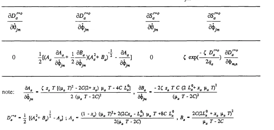
Table 2.2 Approximate expressions for the derivatives of the random plus oversaturation components for upstream links...63

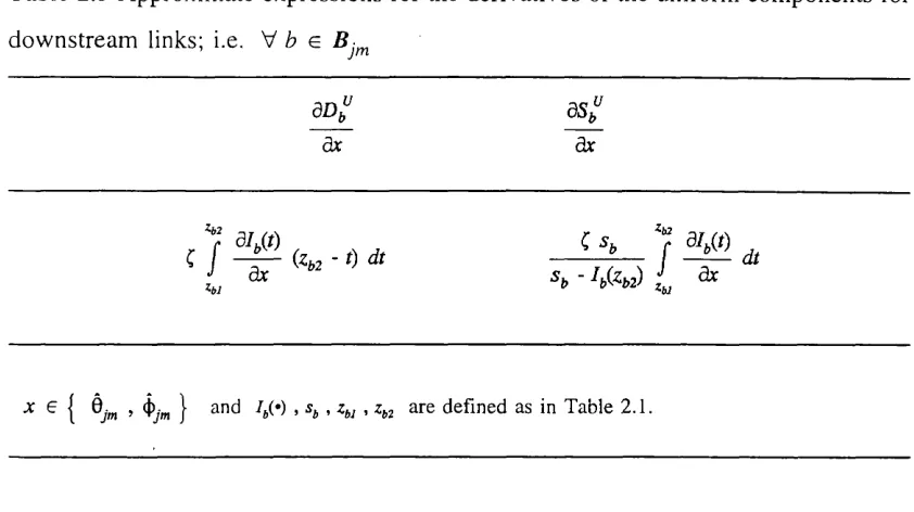
Table 2.3 Approximate expressions for the derivatives of the uniform components for downstream links... 64

Table 2.4. The changes in the IN pattern on downstream links...64

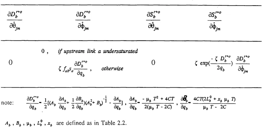
Table 2.5 Approximate expressions for the derivatives of the random plus oversaturation components for downstream links... 65

Table 2.6. Approximate expressions for the derivatives of the uniform components for further downstream links... 65

Table 2.7 Approximate expressions for the derivatives of the random plus oversaturation components for further downstream links... 65

Table 3.1. Expressions of random plus oversaturation component for each link...79

Table 6.1a Input data for two-junction road network... 159

Table 6.1b Constraints for two-junction network... 160

Table 6.2a Relationship between links used in figure 6.2a and links used in figure 6.2c... 159

Table 6.2b Travel demand for Allsop and Charlesworth’s road network... 162

Table 6.3a Fixed data for Allsop and Charlesworth’s road network... 162

Table 6.3b Constraints for Allsop and Charlesworth’s road network... 163

Table 6.4 Results on two-junction network for Hooke & Jeeves’ method... 167

Table 6.5 Results on two-junction network for mutually consistent calculations...167

Table 6.6 Results on two-junction network for method a... 168

Table 6.7 Results on two-junction network for method b... 168

(9)

Table 6.9 Results on Allsop & Charlesworth’s network at 1st initial signal settings for method a... 172

Table 6.9a Results on Allsop & Charlesworth’s network at 1st initial signal settings for method a. (cont)... 173

Table 6.10 Results on Allsop & Charlesworth’s network at 1st initial signal settings for method b... 174

Table 6.10a Results on Allsop & Charlesworth’s network at 1st initial signal settings for method b (cont)... 173

Table 6.11 Results on Allsop & Charlesworth’s network at 2nd initial signal settings for method a... 175

Table 6.11a Results on Allsop & Charlesworth’s network at 2nd initial signal settings for method a (cont)... 173

Table 6.12 Results on Allsop & Charlesworth’s network at 2nd initial signal settings for method b... 176

Table 6.12a Results on Allsop & Charlesworth’s network at 2nd initial signal settings for method b (cont)... 173

Table 6.13 Results on Allsop & Charlesworth’s network at 1st initial signal settings for mutually consistent calculations... 178

Table 6.14 Results on Allsop & Charlesworth’s network at 2nd initial signal settings for mutually consistent calculations... 179

Table 6.15 Results on Allsop & Charlesworth’s network at 1st initial signal settings for re-run mutually consistent calculations... 180

(10)

List of Figures

Figure 2.1 Illustration for the solutions of bi-level formulation and mutually consistent

calculations... 39

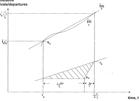
Figure 3.1 Illustration for the uniform component of oversaturated link... 86

Figure 6.1a TRANS YT links for two-junction network... 154

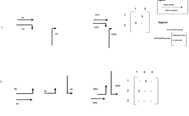
Figure 6.1b Signal groups and clearance time matrices for two-junction network...155

Figure 6.1c Layout of two-junction network represented for use of traffic assignment ...154

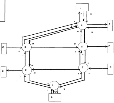
Figure 6.2a Layout for Allsop and Charlesworth’s network... 156

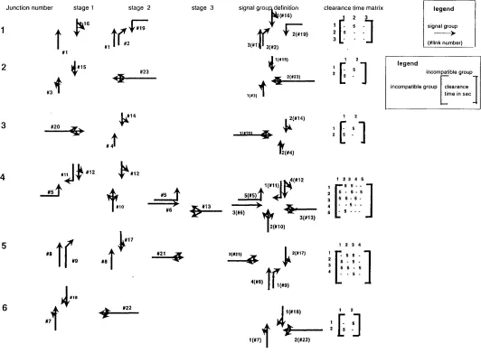
Figure 6.2b Configuration for Allsop and Charlesworth’s road network...157

(11)

Chapter 1 Introduction

1.1 Background

Follow ing the advent of applications of m icroprocessors in traffic signal control, such

applications have achieved practical effectiveness during the last two decades. Firstly,

as far as the scope of traffic control is concerned, it can be classified into the follow ing two ways; isolated junction control and area traffic control. Isolated junction

control assumes that the traffic flow arrival patterns are of Poisson-type distribution w hilst in area traffic control, the traffic flow arrival distribution follows platooning

patterns when the short spacing between adjacent links is considered. Secondly, as far as the way of operating traffic signals is concerned, two methods have been developed: the stage-based control and the phase-based control. Combining the scope

in control and the method of control in a road network, we can have the stage-based isolated junction control, the stage-based area traffic control, the phase-based isolated junction control and the phase-based area traffic control. W ays of optim ising the isolated junction using the stage-based m ethod which can be expressed as a delay- m inim ising convex program m ing have been developed by Allsop (1971). Furtherm ore,

ways of optimising the isolated junction using the phase-based method by adopting sim ilar criteria for the stage-based m ethod have been proposed by Gallivan and H eydecker (1988). On the other hand, ways of optim ising area traffic control using the stage-based method, in which perform ance is expressed as w eighted linear

com binations of vehicular mean delay and num ber of stops per unit time have been developed as a practical traffic study tool for urban networks by Robertson (1969).

M oreover, by applying the traffic model from TRANS YT (Vincent, M itchell and Robertson, 1980) but taking account of a m ore flexible form of control in terms of the

phase-based control variables, W ong (1995) proposed a phase-based optim isation approach for the area traffic control problem .

However, it may be appropriate not ju st to regard the setting of signal timings as sim ply an effective tool in alleviating congested traffic but it may also play a more flexible role to influence the traffic m ovem ents in a preferable way by which the total

(12)

Allsop (1974) noted, ’ when all or part o f the netw ork is subject to trajfic control, the

relationships between travel cost and traffic flo w on some or all o f the links in the

network depend on the control parameters, and the$e can therefore be used to influence the num ber o f journeys made through the network and the routes taken' .

As a result, the area traffic control problem can be com bined with the equilibrium

assignment in such a way that the equilibrium flows are treated as functions of signal setting variables. Considering the fact that the equilibrium flows can be treated as the functions of traffic signal settings, a bi-level mathem atical program m ing approach is

adopted. In dealing with the hierarchical relationships between area traffic control problem and equilibrium traffic assignment, the upper level problem is the area traffic

control problem while the lower level problem represents the equilibrium assignm ent which is a constraint of the area traffic control problem.

By com bining the two problems into a bi-level problem , there are some m athem atical difficulties that result. Firstly, in the upper level problem , the objective function for the area traffic control optimisation with equilibrium network flows needs to be specified as an explicit mathematical expression, in which the chosen indicators for the system perform ance can fully represent the practical travel cost incurred by traffic where the objective function is to minimise the total travel cost. Secondly, in the low er level problem, the travel time function of traffic flow and signal setting variables for each link needs to be decided, which corresponds to the average travel cost incurred

by the traffic at the end of the link controlled by the signal settings. Furtherm ore, the relationship between the equilibrium flows and signal setting variables forms a non

linear constraint on the choice of signal setting variables, which needs to be taken into account as the following solution methods being developed for the bi-level problem .

Thirdly, the ways of searching for a locally optimisation for this bi-level problem need

to be decided in accordance with the following aspects.

!. For given signal settings, to find a descent direction along which the values of the

objective function are consistently decreasing, where the chosen indicators for the system performance are to minimise the total travel cost for all users in the signal-

(13)

2. Along the descent direction for given signal settings, the optimal value of the objective function for the bi-level problem can be obtained by any convenient one dimensional search program m ing technique.

3. A globally optimal search for the minimal value of the objective function for the

bi-level problem can be achieved in this way if the bi-level problem is a convex program m e with respect to signal setting variables; otherwise where the bi-level

problem is a non-convex program m e with respect to the signal setting variables, only a local optimum can be obtained.

4. In the latter case, the feasible search directions can be found in which unconstrained steps can be made to carry the search for better local optim a to many parts of the feasible region.

1.2 Objectives

Therefore, the objectives of this thesis in dealing with the area traffic control optimisation with equilibrium network flows represented as a bi-level problem can be identified in the following way.

1. To form ulate a bi-level m athem atical problem which specifies the area traffic control problem as the upper level problem and user equilibrium traffic assignm ent as

the lower level problem.

2. To define the objective function in the upper level problem in terms of convenient mathematical expressions with respect to signal setting variables and to identify the link travel time function for user equilibrium traffic assignm ent in the lower level

problem.

3. To obtain the derivatives for the indicators of the system perform ance for the b i

level problem and carry out a sensitivity analysis, in which the consequential changes on the equilibrium flows caused by changes of the signal setting variables are

estimated.

(14)

for the indicators of the system perform ance with respect to the signal setting

variables,-in which the descent direction needs to be obtained so that the values of the objective function are consistently decreasing.

5. To identify the optimal step length along each descent direction so that the locally optimal value of the objective function can be obtained.

6 . To develop good search strategies for the better local optim a for the bi-level

problem of area traffic control optimisation and equilibrium flows so that a global search can be carried out in many parts o f the feasible region and the poor local solution can be avoided.

7. To illustrate the effectiveness of the solution m ethod to the bi-level problem of the area traffic control optimisation for equilibrium network flows on test road networks,

and to dem onstrate the effectiveness of the solution m ethod by comparing the values of the chosen indicators for the system perform ance with those obtained by other solution methods.

1.3 Structure of the Thesis

The remainder of this thesis can be organised in the following way.

In Chapter 2, a detailed review of work on the com bined problem of the area traffic control optimisation and user equilibrium traffic assignm ent is given. In relation to the

bi-level formulation of the area traffic control optim isation with equilibrium network flows, formulations of both the upper level and low er level problems are given in Chapter 3. In Chapter 4, a sensitivity analysis for the bi-level problem with respect to

signal setting variables is given, in which detailed expressions for each term in the chosen, indicators for the system perform ance of the bi-level problem are discussed.

In Chapter 5, solution methods to this bi-level problem of area traffic control

optimisation for network equilibrium flows are given and the corresponding search strategies for the bi-level problem are discussed as well. In Chapter 6, numerical

(15)

discussed as well. Conclusion for this thesis and future recom m endations are given in

(16)

Chapter 2 Literature Review

2.0 Introduction

The optimisation problem of area traffic control has been studied over the past few decades. The TRANSYT model proposed by Robertson (1969) has been widely recognized as one of the most useful tools in studying the optimisation of area traffic control. Furthermore, due to recent advanced technologies on the development of microprocessors applied to the operation of signal control, new approaches for studying signal control in urban road networks have been greatly encouraged. For example, a phase-based optimisation approach to the individual signal-controlled junction, which is designed directly in relation to the practical operation of signal groups, has been shown to be successful in achieving better system performance in comparison with previous ways. On the other hand, modelling in relation to users’ behaviour in terms of choice of routes has also been widely researched over the past few decades. However, as it has been noted (Allsop 1974; Gartner 1976) a full optimisation process needs to be applied where the two individual problems are both relevant: the area traffic control optimisation with user equilibrium traffic assignment. The way of dealing with such a combined optimisation problem can be actually regarded as an equilibrium network design problem (Marcotte

1983; Heydecker 1986).

(17)

2.1 Optimisation of Area Traffic Control

2.1.1 The TRANSYT model

TRA N SY T (TRAffic Network Stud Y Tool) is a stage-based optimisation programme including a numerical model of traffic movement in which platooning of vehicular movements between adjacent Junctions is a central feature; the TRANSYT model was invented by Robertson (1969). The performance index in TRANSYT is the sum for all signal-controlled traffic streams of a weighted linear combination of estimated rate of delay and number of stops per unit time which are each evaluated by the numerical model of traffic movement and a simple analytical expression. In TRANSYT, there are two main modules: the traffic model and the signal optimiser; the signal optimiser is the optimisation procedure adjusting signal control variables by repeated evaluation of the traffic model so that the performance index is approximately minimised. The aim of the TRANSYT programme is to find good signal settings for a road network under coordinated control by adjusting the signal settings repeatedly in such a way that only changes in settings that reduce the performance index are adopted. A signal-controlled traffic stream is the basic element for the calculation of signal settings, which either can represent traffic in one or more lanes leading to a junction and used by vehicles in taking a particular movement or can represent for one or more lanes leading to a junction and used by vehicles in taking different movements in such a way that each of the movements shares a lane with one of the other movements. Each traffic stream is in turn represented by its own link in a node link network with one node for a signal-controlled road junction in relation to the definition of the following performance index.

Let L be the set of links, W be overall cost per average vehicle-hour of delay, K be

overall cost per vehicle-stop, and for each link a in L : let be the delay rate in

vehicles, be the number of vehicle-stops per hour, and be respectively

link-specific weighting factors for delay rate and number of stops per unit time. Then the performance index used in TRANSYT is given as

E (M'' «'a K S ,) (2. 1)

a e L

(18)

classified into two components according to the assumption of periodic traffic movement on a cycle by cycle basis and additional random variations resulting from variations in vehicle movements from cycle to cycle: the uniform component of delay rate and of number of stops per unit time, which results from the assumption of identical vehicle arrivals cycle after cycle, and the random plus oversaturation component of delay rate and of number of stops, which results from the random variations in vehicle arrivals and assumption of steadily increasing oversaturation queues when the mean link arrival flow exceeds its capacity.

In calculations of the uniform component for any one link, the common cycle time for the whole road network can be divided into a number of equal intervals called ’steps’. Robertson employed the following three types of flow pattern as functions of time in the cycle in describing the movement of traffic on a link in terms of cyclic flow profiles: (i). the IN profile is the pattern of traffic at the downstream end of the link that would arrive if the traffic were not stopped by the signals.

(ii). the GO profile is the pattern of traffic that would leave the stop line if there was enough traffic to saturate the green.

(iii). the OUT profile is the output pattern of traffic that leaves the link, and is derived from the IN and GO profiles.

For the purpose of deriving the IN profile at the downstream link,which results from the OUT profiles from relevant upstream links, the following recursive expression is used.

+ (1 . (2.2)

where is the flow in the step of the IN profile, g is the flow in step 1: of the OUT

profile from a relevant upstream link, / is the proportion of the OUT flow from that link

which enters the link being considered, and t is 0.8 times the mean undelayed travel

time' (measured in steps) over the distance for which dispersion is being calculated, and

F -

i

is a smoothing factor. 1 4- 0.35 t

(19)

In addition, as for calculations for the random plus oversaturation of delay rate, D and

of the number of stops per unit time, S , simple analytical equations are used

(Vincent, Mitchell and Robertson 1980, pp7-8).

D = I [((? - + {q - M)]

T) r+o S = 2 9 (1 - exp ( _ --- ))

(2.3)

-))

I c q

where c is the common cycle time of the network, q is the average arrival flow, p is

the absolute capacity at the downstream stop line as estimated by the GO pattern, and T is

the period over which the estimate is made.

(20)

In the TRANSYT programme, the traffic movements are represented by a numerical simulation model and no explicit mathematical expression is used. Since the perform ance index is a non-convex function, only a local minimum can be obtained during the hill- climbing search process. In order to reduce the possibility of missing out a good local solution, the TRANSYT programme includes a mixture of both small and large numbers of steps in searching by changing the signal setting variables. For example, TRANSYT uses various numbers of steps in searching by changing the offset variable since there is no limitation over the search region of the offset variable. In addition to changing offsets by various numbers of steps, the TRANSYT programme considers a finer search in changes one of step for the start time of each stage at each junction. As a result, the hill-climbing search process in the signal optimiser of TRANSYT employs a flexible way of adjusting each kind of signal setting variable and by this means an approximation to the global minimum may be found.

In relation to another signal setting variable at the network level, the common cycle time, which is specified as taking a common value for all junctions of the road network (or a submultiple of the common value for some particular junctions), the TRANSYT programme has yet to take account of it as a decision variable in the optimiser. However, the TRANSYT programme evaluates a wide variety of common cycle times on the basis of green times calculated for individual junctions and arbitrary offsets. For example, TRANSYT 8 (Vincent et a i, 1980) provides the information for a wide choice of cycle times, including the corresponding highest degree of saturation and green-time distribution at each junction, the values of performance index for all relevant links, and also options for double cycling at some particular junctions.

2.1.2 Phase-based Optimisation

Another approach to an area traffic control optimisation problem is the phase-based optimisation approach which takes full advantages of higher flexibility provided by recent development on microprocessor controller technology. Optimisation techniques for calculating signal settings using the phase-based optimisation approach deal with the signal control variables in relation to sets or groups of signals: those which are switched

(21)

In this approach the orders of occurrence of stages and the structures of the interstages can be decided automatically during the optimisation process. It has been reported (Silcock and Sang 1989; Silcock 1992,1997) that considerable advantages can be achieved in the system performance by means of the phase-based approach in comparison with the system performance achieved by means of the stage-based approach when applied to individual signal-controlled junctions. In the phase-based approach the signal control variables for a road network; a sequence of stages, durations of stages, structures of interstages, offsets and even common cycle times, can be decided within the optimisation process. Detailed examples and discussions for the advantages provided by this phase-based optimisation approach at individual junctions are given by Heydecker and Dudgeon (1987), Gallivan and Heydecker (1988) and Allsop (1992).

Furthermore, optimisation techniques using the phase-based approach to the area traffic control problem have been investigated over recent years. Firstly, Heydecker (1996) proposed a complementary approach to the area traffic control optimisation problem, in which the results obtained for individual signal-controlled junctions using the phase-based approach are combined with the optimisation of the road network where the network level decision variables such as the offsets and common cycle time are to be taken into account. Such a complementary approach to the area traffic control optimisation problem can be decomposed into two separate levels when carried out in practice: firstly, the individual junction level, in which the structures of interstage and the order of stage occurrences for each individual junction can be optimised according to various choices of criteria; secondly, the network level, in which a full optimisation can be carried out for the system performance of the road network with respect to the durations of stages and the offset variables while the common cycle time, interstage structures and stage sequences are supposed to be fixed at this network level.

(22)

individual junction and network levels. However, because only the critical movement of each signal group is taken into account, the choice of the criterion of the minimum cycle time or the maximum capacity will give rise to some degree of indeterminacy in signal settings. On the other hand, the interstage structures and stage sequences optimised by the criterion of minimum delay rate will not normally achieve equally appropriate effects at the individual Junction and network levels, which is due to the nature of the assumptions about vehicle arrivals, but the corresponding signal settings are fully determined by the optimisation process. After the individual junction decision variables, i.e. the interstage structures and stage sequences, have been optimised, the common cycle time for a road network can be decided in the following way. First, the TRANSYT programme is run with the interstage, structures and stage sequences provided by optimising at the individual junction level, and the common cycle time is chosen as the one with the best value of system performance within the possible range of cycle times, which can be identified by the cycle time selection results in the TRANSYT output. The interstage structures and stage sequences are then optimised again with the chosen common cycle time for each individual junction. If the resulting interstage structures and stage sequences are mutually consistent with the common cycle time, then the optimisation of the individual junction level is complete; otherwise, more iterations will be needed for the determination of the common cycle time, interstage structures and stage sequences.

At the network level, as it is mentioned above, a full optimisation is then carried out for the remaining decision variables, i.e. the durations of stages and offsets, while the common cycle time and the individual junction decision variables remain fixed. If the resulting performance of each junction appears satisfactory, the optimisation at the network level is then regarded as complete; otherwise, further adjustments of signal setting variables are made at the individual junction level and the whole optimisation process is performed again.

(23)

delay rate and number of stops per unit time as in TRANSYT. The mathematical programme can be solved by an integer programming method which is mainly influenced by the derivatives of the value of the performance index with respect to the phase-based control variables. Wong (1995) showed that these derivatives of the performance index as estimated by approximate expressions were in a good agreement with results of numerical differentiation in the case of a test road network. In relation to the use of the phase-based optimisation approach to formulating an area traffic control problem, the following formulations are introduced.

Let c be the common cycle time, and N j be the number of signal-controlled junctions

in the road network. For each signal-controlled junction m, \< m < N j , let be the

number of signal groups and 0^^^^ , (|) - be respectively the start and duration of green for

signal group ; , 1< 7 < ; furthermore let \j> = \j/,„ , 1 < m < Ay ] and

^ m - [ ’ 4)ym : 1 ^ 7 ^ ] • As far as the constraints for the signal control

variables are concerned, we let A = l < m < A y j be a diagonal supermatrix with

matrices A ,,,, 1 < m < N j which are the coefficient matrix with respect to the signal

control variables, and Uq , be respectively coefficient and constant vectors for the

common cycle time c , and a = 1 < m < Ay j , 6 = ^ b 1 < m < A y j be

respectively the coefficient and constant vectors for signal control variables.

Then the area traffic control problem with unspecified common cycle time can be formulated as to

Minimise

subject to «0 0 <

a A b

(2.4)

(24)

Similarly, the area traffic control problem with specified common cycle time can be formulated as to

Minimise f

subject to (2.5)

A \\f^ < b

where b = b - c a

The objective functions -^i(¥) in (2.4)-(2.5) take the following form as shown

in expression (2. 1)

a s L

where D^= D^+ is the delay rate on link a, the sum of the uniform and random plus

oversaturation components of delay rate on the link, and S = S^+ is the number of

stops per unit time on link a, the sum of the uniform and random plus oversaturation components of number of stops per unit time on the link.

In relation to the solution methods to the optimisation problems in (2.4)-(2.5), Wong employed an integer programming method to solve the optimisation problems, which can be divided into two components: the integer linear sub-problem which aims to find a feasible integer direction on the basis of the values of derivatives of performance index with respect to the phase-based signal control variables, and the sub-problem which aims to find the maximum of move size along the feasible direction.

For any one set of initial signal settings, \j/^ = [ , \]/^ ] , the integer linear sub

problem for the area traffic control optimisation problem (2.5) with specified common cycle time is described as follows.

<Integer linear sub ■prohlem>

(25)

Minimise V d ^ d

T " /

subject to A d < b

- 1 < d < 1

r-0

(2.6)

where V is the gradient evaluated at \\P of , which has been reported in

Wong (1995), and b - b - A •

<Sub-problem>

Find integer a to

Minimise f + a d)

a

subject to 0 < a <

(2.7)

where c c ^ = Minimise b,

M

CC; =

M

j - 1

, i e | i ; dj > Q

and M =

m -1

For any one set of initial signal settings, \\f^ = [ , \{/^ ] , and given changes A c the

integer linear sub-problem for the area traffic control optimisation problem (2.4) with

unspecified common cycle time is described as follows.

<Integer linear sub-problem>

Find direction d in the \\f space to

On j T

Minimise V PqÇv/ ) d

d

subject to A d ‘ < b

- I < d < I

(2.8)

(26)

d P n

been reported in Wong (1995), with the first element ___ omitted, and

Ù = b - A (\|/^)^ - a (c^ + A c )

<Sub-problem>

Find integer a to

Minimise + a d)

a

subject to 0 < a <

where d = [ A c , ]

A c

let «Q = '

A c

, if A c > 0

if A c < 0

if A c = 0

where c • , c are respectively the minimum and maximum cycle time.

(2.9)

M

b, - a, ?» - Ç A,j Minimise ) «q , Minimise ) 0L ^ =

---M

A c + Ay dj

7-1

M

i e j Î ; Cj. A c + ^ Ay dj > 0

I 7-1

where M = 2 ^ N

m " I pm

(27)

hill-climbing search process in TRANSYT with the integer programming method. The optimisation process consists of two classes of optimisation steps: a network-wide optimisation step, changes all signal control variables simultaneously over the road network aiming to approach the neighbourhood of a good local optimum, and a junction-based optimisation step, which changes the signal control variables junction by junction aiming to fine-tune the timings at each junction. This optimisation process for the area traffic control problem for any given set of initial signal settings can be summarized in the following steps.

Steps 1&2: Use a combination of large and small step sizes for the adjustments of the offset variables, which is the same procedure as implemented in the hill-climbing search process as in TRANS YT, such that a good initial solution can be obtained.

Step 3: Adjust the common cycle time and green times by changing the signal control variables simultaneously by means of the integer programming method, which is implemented by the network-wide optimisation step.

Steps 4&5: Repeat Steps 1&2 to find another better local optimum.

Step 6: Reduce the move size into one unit interval for the adjustment of offset variables to locate the neighbourhood of the local minimum.

Step 7: Reallocate green times by implementing the integer programming method on the junction-based step and changing the green times junction by junction.

Step 8: Repeat Step 6 for final checking in the search for the near-global optimum.

2.2 User Equilibrium Traffic Assignment

(28)

destination. As it has been enunciated by Wardrop (1952), a user equilibrium traffic assignment can be described as follows.

" The journey times on all the routes actually used are equal, and less than those which would be experienced by a single vehicle on any unused route. "

For a given number of origin-destination trip rates over a period of analysis, the resulting equilibrium traffic flows and the corresponding travel times can be calculated by solving an equivalent mathematical programme. Beckmann, McGuire and Winsten (1956) first proposed an equivalent user equilibrium mathematical programme, in which the solutions satisfy the conditions required by the user equilibrium traffic assignment. Furthermore, a unique solution to the user equilibrium programme can be obtained when some strict mathematical conditions are satisfied by the link travel time function. In relation to the equivalent user equilibrium mathematical programme, the mathematical formulation will be given first, and the corresponding characteristics of the solutions will be discussed later.

2.2.1 Equivalent mathematical programme to user equilibrium assignment 2.2.1.1 Beckmann transformation

The formulation of the user equilibrium programme according to Beckmann transformation is as follows.

Let L be the set of links, W be the set of origin-destination pairs, and be the set

of paths between each origin-destination pair w , V w e VF .

Let 5 = [ ^a/; ] be the link/path incidence matrix where 0^^ = 1 if link a is in path

p , and 5 = 0 otherwise, V a E L , V p E F ^ ^ , V w E VF , and A = J ] be

the origin-destination/path incidence matrix where A^^^ = 1 if path p connects origin-

destination pair w , and A^^^ = 0 otherwise, V /7 e F ^ , V w e V F .

(29)

in W , f = [ //, ] be the row vector of all path flows, and q = [ ] be the row

vector of all link flows.

Let c{q) = J ] be the row vector of link travel times, in which denotes

the link travel time depends only on the flow on that link, i.e., separable relationship

between the link travel time and corresponding flow is assumed, and C{q) = J C^J^q) j be

the row vector of path travel times.

Then the equivalent programme is to

Minimise Z{q) = j c^(vv) dw

q a e L 0

subject to Y . f p = D ^ , \ f w e W ^

P ^

E E f p ^ a p = ^ ^ ^ ^ ^

w e W p €

y;, > 0 , V p e , V w e w

Furthermore, the dependence of link flows q on path flows / and the dependence of path

travel times C{q) on link travel times c{q) can be expressed in terms of the incidence

matrix as follows.

9^ = 6 / ^ (2.11)

C ( q Ÿ = & ' ^ c ( q f (2.12)

2.2.1.2 Equivalent conditions for user equilibrium programme

(30)

the network is in user equilibrium. Following this equilibrium conditions, the first-order necessary conditions for the mathematical programme (2 . 10) have been shown equivalent to the equilibrium conditions for the user equilibrium traffic assignment (Sheffi, 1985, pp 63-66). The first-order necessary conditions for (2.10) can be given as follows.

( q , - « j = 0

q ,

■ “ w

- 0

/ „ s o

E f„ = , V w e tv

(2.13)

(2.14)

P e P „ ,

where is the minimum path travel time for specified origin-destination pair w,

V w 6 W .

Expressions (2.13)-(2.14) show that for all used paths carrying traffic flows the corresponding travel times equal the minimum travel time while for any unused path carrying no flow, the corresponding travel time is not less than the minimum travel time. Therefore, that can be expressed in the following statements.

q, =

.

i f f p >

0 q s

, i f f p = 0

, V p e P V w e i y (2.15)

2.2.1.3 Uniqueness condition for user equilibrium programme

The uniqueness condition for the user equilibrium programme with respect to link flows shows only one solution that minimises the objection function (2. 10) and the solution also satisfies the equivalent conditions in expressions (2.13)-(2.14) if and only if the strict convexity condition of the user equilibrium programme with respect to link flows is satisfied.

(31)

links. Furthermore, for the reasons of traffic congestion on the road network, it assumes that the link travel time will increase strictly as the corresponding flow increases. In relation to mathematical expressions, both the assumptions of separability and strict increase of link travel time due to traffic congestion can be given below.

^ Q b * a , V a , b e L ‘Ih

‘‘ Cg(‘la)

d ‘I n

(2.16) > 0 , V a E L

Following the assumption in terms of expression (2.16), it can be seen that the Hessian matrix of the equivalent programme is a diagonal matrix with strictly positive diagonal elements and hence positive definite; therefore the solution to the user equilibrium programme (2.10) (i.e. the solution that satisfies the equivalent conditions (2.13)-(2.14)) is unique.

Following the equivalent user equilibrium programme, a general formulation for the user equilibrium traffic assignment can be formulated in terms of a variational inequality problem by Smith (1979).

2.2.1.4 Variational inequality problem formulation

A general formulation for a user equilibrium traffic assignment problem can be expressed in terms of a variational inequality problem as shown by Smith (1979) and identified by Dafermos (1980).

To find values q * o f q such that

c(9*)(« - ? * ) ^ > 0 (2.17)

V q € a = { q - q ' ^ = 5 / ^ , A / ^ = D ^ , / > o }

2.2.2 Solution method to user equilibrium traffic assignment

(32)

the basis of current travel times in deciding a feasible direction along which the value of objective function of (2.10) subject to constraint set can be reduced. Second, a sub- programme is formulated, in which the optimal move size along the feasible direction can be decided and hence the value of the objective function is minimised. In the linear programme, the first derivatives of the objective function with respect to path flows are used to determine the minimum path travel time for specified current traffic flows. This step is no more than a shortest path problem, in which the all-or-nothing traffic assignment is carried out in search for auxiliary flows on the basis of current travel times. In the sub- programme, a one-dimensional optimisation problem is carried out for which an optimal move size can be decided such that the value of objective function in terms of a linear combination of current flows and auxiliary flows is minimised. The linear programme and the corresponding sub-programme for the convex combination method can be carried out alternately in a series of iterative processes until a required criterion is satisfied.

<Linear programme>

Let be current link flows at iteration n and c , C be respectively current link

and path travel times at iteration n .

Find the shortest path at iteration n between each origin-destination pair w in W based

on current traffic flows to

Minimise ^ ^ C ^

/ w e W p &

subject to

^

, y w e W

P G Pvv

/ “ > 0 p e P „ , V w e W

The linear programme (2.18) iS to find the shortest paths with the smallest travel times

at iteration n . i.e. = \ ^ for v/hich the travel demands of all origin-destination

(33)

flows and the corresponding current travel times c and C . In other words,

the resulting traffic assignment is no more than a problem of finding the shortest path for given specified travel time and thus it can be performed by the technique of all-or-nothing traffic assignment. The all-or-nothing traffic assignment for programme (2.18) can be described as follows.

For each origin-destination pair w in W and given trip rate over a period of analysis,

Ù , there exists a path h connecting origin-destination pair vu at iteration n , such

that

f T = . if , V p e

and = 0 , \f p ^ h

The corresponding auxiliary link flow can be derived in terms of the link-path

incidence matrix.

( « '" T = 5 y c y (2.19)

<Sub-programme>

Following the auxiliary flows q^f* obtained by expression (2.19), a one-dimensional line

search to find the optimal move length along the descent direction,

d = q^!^^ - q^Q^ which minimises (2 . 10) is to

Minimise Z(ç^^ -I- {q^f^ - ^[j^^))

(

2

.

20

)

subject to 0 < < 1

(34)

One of solution methods to a one-dimensional optimisation problem is a Bolzano search- bisection method. When this is applied to (2.20), the optimal move size can be found if the following condition is met.

= 0

0 < < 1 (2.21)

where - g^^)

The (2.21) corresponds to the ’cost equilibration’ as mentioned by Van Vliet (1987). When the sub-programme is solved by using a one-dimensional search process, new traffic flows can be obtained by the linear combination of auxiliary and current flows by means of the optimal move size and then the corresponding travel times can be updated accordingly. In relation to the stopping criterion for the convex combination method when carried out in a sequence of iterative processes by solving alternately the linear programme and sub-programme, it is suggested (Sheffi, 1985, p p ll9 ) to stop when the difference in the total origin-destination travel times between successive iterations is not greater than a predetermined threshold value, i.e..

E

e W

- 4 " - "I

. (n) <

8 (2.22)

where is the minimum travel time between a specified origin-destination pair w in

W at iteration n , which can be found by (2.18), and e , e > 0 , is a predetermined

value of threshold.

(35)

Step 0: Initializ.ation.

0.1 Set indicator n = 0 .

0.2 Perform all-or-nothing traffic assignment based on current travel times,

c = 0) by solving the linear programme (2.18) and yield the corresponding link

flows .

0.3 Set indicator n = \ .

Step 1: Update.

Set c = c

Step 2: Direction finding.

Perform all-or-nothing traffic assignment based on by solving the linear programme

(2.18) and yield the auxiliary link flows by means of (2.19).

Step 3: Line search.

Find along the descent direction d - q^^^ by solving (2.20), which also

can be carried out by means of (2.21).

Step 4: Move.

Set ^ + «<")

Step 5: Convergence test.

If condition (2.22) is met then the convex combination procedure is complete and

(36)

2.3 Equilibrium Network Design Problem 2.3.1 Introduction

In Section 2.2, a user equilibrium traffic assignment has been formulated as an equivalent mathematical programme given by fixed travel demands during a specified time of analysis for a general road network represented in terms of a number of nodes and links. In a general road network, when some or all nodes are subject to signal control, the travel time function for each link needs to be expressed in a form in which the average delay incurred by traffic at the downstream junction can be taken into account. Furthermore, it has been widely recognized (Allsop 1974, Gartner 1976) that the resulting equilibrium flows and the corresponding travel times in a road traffic network are strongly influenced by the operation of signals. Therefore, a revised equivalent user equilibrium programme can be expressed in the following way when the signal setting variables are taken into account in the link travel time functions. Recall the Beckmann transformation (2.10) for an equivalent user equilibrium programme, in which (2 . 10) can be revised as follows when signal settings are taken into account in the equilibrium flows and the corresponding travel time functions.

For any given signal settings \\f , a revised equivalent mathematical programme to the

equilibrium traffic assignment when signal settings are considered is to

Minimise Z^(g , Ÿ) = ^ j* , w) dw

9 a e L Q

subject to 2 , V w e W ^2,23)

E

^ap

**” «.(*) . V a 6 L**

w e W p e

/ / t ) ^ 0 , V p e P ^ , V w e W

Recall the generalized formulation given by fixed travel demands, D , during a specified

time of analysis, for which the user equilibrium traffic assignment is in terms of a variational inequality problem, (2.17) can be revised as follows when signal settings are taken into account in the equilibrium flows and the corresponding travel time functions.

(37)

c(q* , i|>) («(♦) - i 0 (2.24)

V ,( $ ) e Ü (*) = { ,( $ ) ; «(i|r)'’ = Ô / ( ♦ ) '', A

f(qff

= 0 % ^ 0 }

As it is noted in expressions (2.23)-(2.24), given by the fixed travel demands, D , of all

pairs of origin-destination during a specified time of analysis, the resulting equilibrium

flows and the corresponding travel times depend on the signal setting variables, \\f .

Therefore, for a road traffic network subject to signal control operation, the sequential effects on the resulting equilibrium flows and the corresponding travel times will be caused if any element of the signal setting variables varies. In Section 2.1, the optimisation problem of area traffic control has been reviewed, in which we supposed the average traffic flow patterns remain fixed while the signal settings are optimised. This assumption can be relaxed now and a full optimisation process can be performed by which the problem of the area traffic control optimisation and the problem of user equilibrium traffic assignment are brought together as a combined optimisation problem. In addition, this combined optimisation problem can be regarded as one special case of the equilibrium network design problem.

(38)

the ways of formulating the equilibrium network design problem for the area traffic control will be introduced first and the corresponding solution methods will be discussed accordingly.

2.3.2 Formulations

The mathematical optimisation formulation is to achieve the optimal value of the objective function with respect to decision variables of interest, in such a way that the dependence of equilibrium traffic flows on signal settings is taken into account. The optimisation formulation applied to the area traffic control problem while user equilibrium flows are assumed is described in the following way.

Let \\f be the signal settings, q *(\{/) be the corresponding equilibrium flow which can

be obtained by solving (2.23) or (2.24), and Sq be the feasible region for signal settings.

Find the signal settings \\f within the feasible region Sq to

Minimise Zq(\]/ , ^ *(\J/))

(2.25)

subject to \\f e Sq

Furthermore, the mutually consistent formulation for the optimised area traffic control problem and user equilibrium traffic assignment can be expressed as follows.

To find y * such that

22(4/* , q *(4/*)) = Minimise Z2(vg , q *(\{/*))

^ (2.26)

subject to \(/* G Sq

In (2.26), the objective of the formulation for mutually consistent signal settings and the

corresponding equilibrium flows is to find a particular signal setting v/* which

minimises the value of the objective function, Z2(\|/* , g *) , which is in terms of chosen

(39)

for the area traffic control optimisation problem and equilibrium network flows, in which the signal settings and link flows were treated alternately and obtained respectively by solving the area traffic control optimisation problem for the assumed link flows and by solving user equilibrium traffic assignment for the resulting signal settings until an intuitively expected convergence is achieved. The resulting mutually consistent signal settings and link flows will, however, in general be a non-optimal solution as has been discussed by Gershwin and Tan (1979) and Dickson (1981).

On the other hand, in relation to the ways of the mathematical formulation for (2.25), the bi-level formulation has been adopted as an appropriate tool in dealing with this combined problem. For example, Heydecker and Khoo (1990) formulated this combined problem as a bi-level programme, in which the optimisation of signal timings was regarded as the upper level programme whilst the user equilibrium traffic assignment was regarded as the function of signal timings and therefore it was dealt with as the lower level programme. In the bi-level formulation to the optimisation for area traffic control and equilibrium network flows, it is recognized that although the link flows must be in equilibrium for the resulting signal timings, the signal timings will not in general be optimal for the resulting link flows if the latter are regarded as fixed. In comparison with the results obtained from the mutually consistent formulation (2.26) in a trial road network, it was reported that as expected the total system performance achieved by the bi-level formulation was an improvement on that given by mutually consistent formulation (Heydecker and Khoo 1990).

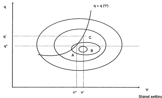
The approaches of the bi-level formulation (2.25) and mutually consistent formulation (2.26) for the equilibrium network design problem can be illustrated (Allsop 1997) by the two-dimensional contours in Figure 2.1. In Figure 2.1, the two-dimensional contours

represent the signal settings \}/ and the corresponding link flows q that give particular

values of performance index. For example, the inner contour represents a smaller value of the performance index than does the outer contour. The objective is to find the minimum value of the performance index represented by the two-dimensional contours by adjusting

the signal settings \|/ and the corresponding equilibrium flows q . The curve ^(\j/)

(40)

Sink flow s

ijj

_Q

q

q*

Signal settings

(41)

optimal signal settings ty* and the corresponding equilibrium flows q * = ^(\{/*) .

Taking the optimal equilibrium flows q * = the fixed value for the next step

in searching for the mutually consistent solution, we may find that the optimal signal

settings move from Y* to \s/ and the solution point moves from point A to B . Given

the mutually consistent signal settings \\f as the fixed value, the corresponding equilibrium

flows can be solved by the user equilibrium traffic assignment (2.23) or (2.24) and

represented by ^ = ^(\}Z ) corresponding to the point C with a rather higher value of

the performance index contour. Since optimising signal timings for this equilibrium flows

will make little difference to \\f we see that , q is an approximate solution to the

mutually consistent formulation (2.26), which is quite far from the optimal solution, i.e.

\\f* , q * given by (2.25).

2.3.3 Solution methods

In relation to the solution methods to the equilibrium network design problem for area traffic control, there are two classes of solution method according to the corresponding formulations: the mathematical optimisation method and the mutually consistent calculation. As it is noted in (2.26), Allsop and Charlesworth (1977) and Charlesworth (1977) reported a mutually consistent calculation for the signal settings in a test road network and the corresponding equilibrium traffic flows. The mutually consistent calculation of signal settings and the corresponding equilibrium traffic flows involved two classes of calculation: one is calculation of the optimal signal settings for an area traffic control problem with fixed traffic flows, and the other is calculation of user equilibrium traffic assignment problem with fixed signal settings.

(42)

this process can be carried out in a series of iterations, where one iteration of the mutually consistent calculation can be stated as follows. First, for the area traffic control optimisation problem when the traffic flows remain fixed, the optimal signal settings which minimised the chosen indicators of the system performance index can be obtained by means of the techniques discussed in Section 2.1, and thus the corresponding average traffic delay occurred at the downstream junction of each link can be specified as a component of the travel time function for further use in the user equilibrium traffic assignment. Second, following the convex combination method as discussed in Section 2.2 to solve the user equilibrium traffic assignment problem (2.23) or (2.24) with specified signal settings and corresponding incurred average traffic delay, the resulting equilibrium traffic flows can be obtained and therefore replace the fixed ones in the area traffic control optimisation problem for next iteration. Mathematical expressions for the alternate calculation for the above two problems can be given as follows.

Minimise Z2(\j/ , q)

^ ^ (2.27)

subject to q = q

and

Minimise Zj(\j/ , q)

(2.23)

subject to \|/ = \}/

where q , ^ are respectively the fixed values of equilibrium flows and signal settings,

and Q (\|/) is the set of user equilibrium flows when the signal settings V|/ is taken into

account.

(43)

To find the optimal value of the performance index for the equilibrium network design problem (2.25), a variety of mathematical optimisation methods have been reported for dealing with the dependence of equilibrium flows on signal settings. As far as these mathematical optimisation methods are concerned, two distinct classes have been noted according to the way of dealing with the dependence of equilibrium flows: firstly, a direct search approach by means of Hooke and Jeeves’ method, which solved an unconstrained optimisation problem with respect to the decision variables where the equilibrium flows were regarded as one of the decision variables; secondly, a bi-level programming approach, which solved a constrained optimisation problem where a two level formulation was considered and the user equilibrium traffic assignment was solved by the lower level problem. In the following paragraphs, we will have a look at the direct search approach to the equilibrium network design problem (2.25) by means of Hooke and Jeeves’ method first; then the bi-level programming approach will be investigated for the application to the equilibrium network design problem.

Dealing with the dependence of equilibrium flows on decision variables can be solved by means of a direct search approach where Hooke and Jeeves’ method (1961) is used. Abdulaal and LeBlanc (1979) reported the formulation and solution method by means of Hooke and Jeeves’ method for an equilibrium network design problem with continuous variables. Since no explicit mathematical expression is available for the relationships of the equilibrium flows to the decision variables, in relation to the application of Hooke and Jeeves’ method to an equilibrium network design problem, Abdulaal and LeBlanc solved an unconstrained optimisation problem in which the dependence of equilibrium flows on decision variables was dealt with as one of the decision variables and solved directly by means of the convex combination method. Following the Hooke and Jeeves’ method, the equilibrium flows need to be calculated each time when a decision variable changes and the value of the objective function will be changed accordingly. As for the application of Hooke and Jeeves’ method to the equilibrium network design problem for area traffic control optimisation in (2.25), the following steps as referred to Abdulaal and LeBlanc (1979, pp32) are given below.

Step 1. Initializ.ation:

(44)

variables for (2.25), choose an initial solution point satisfied the constraint set Sq

in (2.25), and let \\f = .

1.2 Set an initial step size a , a > 0 for the exploratory search in Step 2 and the

acceleration factor |3 for the pattern search in Step 3; set indicator r\ = 1

1.3 Set indices j = \ , k = 0

Step 2. Exploratory search:

2.0 If ./ = + 1 , go to Step 3

2.1 Let eJ , j = 1 A/ be a vector with 1 in the j th component of the decision

variable vector and 0 elsewhere, and set \j/ = \\f + a r\ €j .

Evaluate the objective function Zq at along its positive coordinate direction with

predetermined step move size a .

2.2 If Zq(\|/) < Zq(\|/) put \j/ = Y , J = y + 1 , T| = 1 and go to Step 2.0; otherwise go to Step 2.3.

2.3 If r\ = 1 , put T{ = -1 and go to Step 2.1, otherwise if r\ = -1 put j= j+ 1 ,

r\ = 1 and go to Step 2.0.

Step 3. Pattern search: when the evaluation of the objective function with respect to each component of the signal settings has been conducted in the exploratory search, we need

to compare Zq at and

3.1 If Zq(^) < Zq(V^O , put \]/^ = \jy and \\f = and