Extension of Thin Wire Techniques in the FDTD Method
for Debye Media
Dmitry Kuklin*
Abstract—There are applications of the finite difference time domain (FDTD) method, which need to model thin wires in dispersive media. However, existing thin wire techniques in the FDTD method are developed only for the conductive and dielectric media. The article presents a modification of oblique thin wire formalism proposed by Guiffaut et al. and a minor modification for the technique proposed by Railton et al. for applications with Debye media. The modifications are based on auxiliary differential equation (ADE) method. The modifications are validated by calculations of grounding potential rise (GPR) of a horizontal electrode buried in soil with dispersive properties.
1. INTRODUCTION
For particular simulations, there is a need to take into account frequency dependence of complex permittivity [1]. For example, a recent study [2] shows a significant influence of frequency dependent soil parameters on the grounding potential rise. As long as FDTD method has some strengths (such as modeling of inhomogeneities, for example), it is important to have an opportunity to use the method for calculations with thin wires in dispersive media. However, there is a number of difficulties in approximating the time domain expressions for the complex permittivity by finite differences [6]. On the other hand, there exist well-developed methods modeling Debye relaxation [18] which can be used as an approximation for the complex relative permittivity in a needed frequency range.
One can mark out two groups of techniques modeling thin wires in the FDTD method. In the first group, the FDTD equations for electric and magnetic field calculation are used to model the wire. Correct wire diameter is modeled by altering the FDTD equations [13, 14] or modifying parameters of the medium [15, 16]. The wire itself is modeled by using a high conductivity medium in the electric field calculation nodes locating along the wire (for the ideal conductor the electric field is set to zero in those nodes). In this work, the technique proposed by Railton et al. [16] and improved by Taniguchi et al. [17] is used. In the second group, two additional equations are used to model the current and voltage waves propagating along the wire. The technique was originally proposed by Holland and Simpson [8] and improved by number of authors [10–12]. The oblique thin wire formalism [12] is seemingly the only method to this moment allowing to model arbitrarily oriented thin wires (which radius is not specified by the cell size) in the FDTD method with rectangular mesh. However, in order to use these techniques in Debye media, they need to be modified.
Received 18 August 2016, Accepted 29 September 2016, Scheduled 13 October 2016
* Corresponding author: Dmitry Kuklin ([email protected]).
2. OVERVIEW OF AUXILIARY DIFFERENTIAL EQUATION METHOD FOR DEBYE MEDIA
One of the approaches to model dispersive materials in the FDTD method is the auxiliary differential equation method [7, 18]. This is an efficient algorithm that adds a relatively small amount of floating-point operations and storage needed for unknowns to basic FDTD algorithm. It is convenient to make an overview of ADE method.
Ampere’s law for Debye medium in the frequency domain is
∇ ×Hˆ =0∞jωEˆ +σEˆ +
P
p=1
ˆ
Jp, (1)
where ˆHis the magnetic field, ˆE the electric field, 0 the vacuum permittivity, ∞ the permittivity at
the high frequency limit, σ the conductivity, P the number of Debye poles, and ˆJp the polarization current for thep’th Debye pole:
ˆ
Jp = 0Δpjω 1 +jωτp
ˆ
E, (2)
where τp is the relaxation time, Δp = p − ∞ (where p is the low frequency permittivity).
Multiplication of both sides of Equation (2) by (1 + jωτp) and applying inverse Fourier transform
gives
Jp+τp∂
Jp
∂t =0Δp ∂E
∂t . (3)
In the finite difference form, using Jnp+1/2 = (Jnp +Jpn+1)/2 (time moment is determined as t =nΔt),
Equation (3) can be approximated as Jn
p +Jnp+1
2 +τp Jn+1
p −Jnp
Δt =0Δp
En+1−En
Δt . (4)
Solving this for Jnp+1 gives
Jn+1
p =kpJnp +βp
En+1−En
Δt , (5)
where
kp =
1−Δt/(2τp)
1 + Δt/(2τp), βp
= 0ΔpΔt/τp 1 + Δt/(2τp).
(6)
So that updating of polarization currentJp is performed by Equation (5).
Next, an electric field updating equation should be obtained. Using the Equation (5), Jnp+1/2 can
be evaluated fromEn,En+1 and Jn: Jn+1/2
p =
Jn
p +Jnp+1
2 =
1 2
(1 +kp)Jnp +βp
En+1−En
Δt
, (7)
then it can be substituted into the time domain form of Equation (1) approximated by the finite differences:
∇ ×Hn+1/2=
0∞
En+1−En
Δt +σ
En+1+En
2 +
1 2
P
p=1
(1 +kp)Jnp +βp
En+1−En
Δt
, (8)
and the electric field at n+ 1 can be calculated:
En+1 =
20∞+
P
p=1
βp−σΔt
20∞+
P
p=1
βp+σΔt
En+ 2Δt
20∞+
P
p=1
βp+σΔt
·
⎡
⎣∇ ×Hn+1/2−1
2
P
p=1
(1 +kp)Jnp
⎤ ⎦. (9)
3. MODIFICATION OF THE MODEL PROPOSED BY GUIFFAUT ET AL.
Each method, based on the approach of Holland and Simpson, uses two equations to model propagation of waves along the wire:
L∂I ∂t +
∂V
∂z +RI = Ez(d), (10)
Cl∂V
∂t + ∂I ∂z +
σClV
0∞
= 0, (11)
where I is the current; V is the voltage; Cl,L and R are respectively the capacitance, the inductance
and the resistance per unit length; Ez is the electric field longitudinal to the wire at the distancedfrom
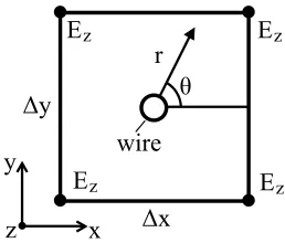
the wire. Applying ADE approach, the second equation is modified and one more equation is added.
Δx
Δy θ
x y
z
r
Ez Ez
Ez
Ez
wire
Figure 1. Thin wire and closest electric field nodes of the FDTD grid.
Figure 1 shows a thin wire oriented along z-axis and closest electric field nodes. The θcomponent of the Faraday’s law in cylindrical coordinates:
∂Er
∂z − ∂Ez
∂r =−μ ∂Hθ
∂t . (12)
Equation (10) is derived by taking the integral of Equation (12) fromr =a(where ais wire radius) to d
d
a
∂Er
∂z −
d
a
∂Ez
∂r =−μ
d
a
∂Hθ
∂t (13)
and substituting approximations for the magnetic and electric field around the wire (hereQis the charge per unit length) [8]:
Hθ = 2I
πr, Er= Q 2πr0∞
= ClV 2πr0∞.
(14)
The RI takes into account the resistance of the wire [12]. The Lis defined by
L= μ0
2π ln(d/a). (15)
Equation (11) is derived from the Ampere’s law in a similar manner as the modified version below (with the exception that the modified version takes into account the polarization current).
The modification starts from the radial component of Ampere’s law equation in cylindrical coordinates:
1 r
∂Hz
∂θ − ∂Hθ
∂z =jω0∞Er+σEr+
P
p=1
Jrp. (16)
Integration of the equation from θ= 0 to 2π yields
1 r
∂ ∂θ
2π
0
Hzdθ− ∂
∂z
2π
0
Hθdθ=jω0∞ 2π
0
Erdθ+σ
2π
0
Erdθ+ P
p=1 2π
0
Using Equation (14) and approximating the derivative∂I/∂zby finite difference, Equation (17) becomes
Ik+1/2−Ik−1/2+jωCV +σCV
0∞
+
P
p=1
Jrp = 0, (18)
whereC is equivalent capacitance for particular nodek (in [12], Ck is used), and Jrp equals
Jrp =
Δpjω
∞(1 +jωτp)CV.
(19)
In a similar manner as earlier, an update equation for theJrp can be obtained:
Jnrp+1=kpJ n
rp+βpC
Vn+1−Vn
Δt , (20)
where
kp = 1−Δt/(2τp) 1 + Δt/(2τp), β
p=
ΔpΔt/τp
∞+∞Δt/(2τp).
(21)
Approximation of time domain version of Equation (18) by finite differences with using Jrnp+1/2 = (Jrnp+Jrnp+1)/2 leads to
−Ikn+1+1//22−Ikn−+11//22
=CV
n+1−Vn
Δt +σC
Vn+1+Vn 20∞
+1 2
P
p=1
(1 +kp)J n p +βpC
Vn+1−Vn Δt
. (22)
Now the voltage at n+ 1 can be calculated:
Vn+1 =b1Vn−b2
C · ⎡ ⎣In+1/2
k+1/2 −I
n+1/2
k−1/2 +
1 2
P
p=1
(1 +kp)Jnrp ⎤
⎦, (23)
where
b1 =
20∞+0∞
P
p=1
βp −σΔt
20∞+0∞
P
p=1
βp +σΔt
, b2 =
20∞Δt
⎛
⎝20∞+0∞
P
p=1
βp +σΔt
⎞ ⎠
. (24)
Accordingly, calculation of the voltage in a multiwire junction [12] should be modified also:
Vn+1=b1Vn+ b2
Ceq,0 ·
⎡ ⎣Nw
q=1
Iqn+1/2−
1 2
P
p=1
(1 +kp)J n rp
⎤
⎦, (25)
where Nw is the number of wires in the junction [12] and Ceq,0 the equivalent capacitance for the
junction [12]. The update equation for theJrp is
Jnrp+1 =kpJ n
rp+βpCeq,0V
n+1−Vn
Δt . (26)
The current from the wire is distributed by the FDTD grid by means of the current sources. Therefore, the electric field at time step n in Equation (9) should be saved before the wire current is distributed. The saved electric field is used then in a calculation of the polarization current by the Equation (5).
4. MODIFICATION OF THE MODEL PROPOSED BY RAILTON ET AL.
The technique proposed by Railton et al. [16] is based on the correction of electric and magnetic fields in the nodes adjacent to the wire. Modeling of the wire itself is performed either by setting the electric field to zero along the electric field nodes or using a highly conductive medium.
According to the technique [16], the permittivity and the permeability in the nodes adjacent to z-directed wire should be multiplied by the coefficients x,y,μx,μy:
μx=
1 y
= ln
Δy
a
2 arctan
Δx Δy
Δx
Δy, μy = 1 x
= ln
Δx
a
2 arctan
Δy Δx
Δy
Δx, (27)
wherea is the wire radius, and Δx and Δy are respectivelyx and y dimensions of the cell. If the wire is located in the conductive medium the conductivity should also be altered [17], and σx=x,σy=y.
To use this technique in Debye media, Δshould be corrected as well by Δx=x and Δy =y.
This can be achieved by alteringβpin Equation (6). As long as in the model of Noda and Yokoyama [15]
the permittivity is corrected in a similar way, the same correction of Δε should be applicable to the model [15] too.
5. VALIDATION
In order to validate the proposed modifications, the calculations of the GPR for a buried horizontal electrode have been carried out by the FDTD method. Then the calculation results have been compared to those simulated using the hybrid electromagnetic model (HEM) which is validated experimentally [5]. First, the complex permittivity should be approximated with the Debye relaxation function. From the empirical expression in the work of [5] the imaginary part of the permittivity can be evaluated:
r(f) =
1.2·10−6σ00.27·(f−100)0.65
2πf 0 ,
(28)
where f is the frequency in Hz and σ0 a soil conductivity (σ0 = 1/ρ0). The frequency range for f in
formula (28) is 100 Hz–4 MHz [5]. The real part of the permittivity [5]:
r(f) = 7.6·103f−0.4+ 1.3. (29)
The frequency range for Equation (29) is 10 kHz–4 MHz. For the range 100 Hz–10 kHz, it is suggested in [5] to use constant permittivity equaled to the permittivity at frequency 10 kHz. However, for the calculations in the present work, the frequency range 10 kHz–4 MHz is enough.
Then-term Debye function expansion is defined by
ˆ
r(ω) =∞+ n
p=1
Δp
1 +jωτp.
(30)
To calculate the parameters∞, Δ, andτ, a hybrid particle swarm-least squares optimization approach
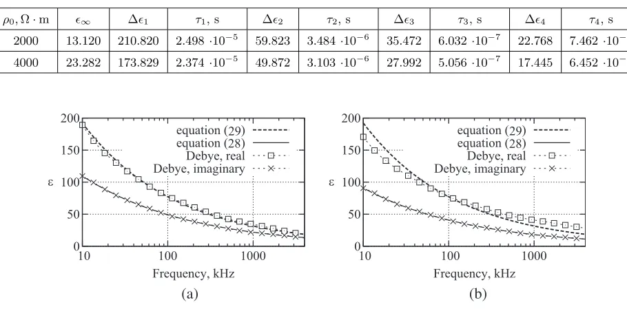
was used [6]. The obtained four-term expansion parameters for the soils with resistivity 2000 Ω·m and 4000 Ω·m are listed in Table 1. Fig. 2 shows the real and imaginary parts of the Debye function expansion compared to those of the empirical functions for 10 kHz–4 MHz frequency range.
It should be noted that the real and imaginary parts of the permittivity are related to each other by the Kramers-Kronig relations [6, 19]. However, Equations (28) and (29) do not obey these relations because the imaginary part depends on the ρ0 while the real part does not (in other words,
the imaginary part of the permittivity is not related to the real part mathematically). For this reason, it is not possible to approximate both equations exactly for all soils by the Debye function expansion (but a good approximation is possible for soils with ρ0 close to about 2000 Ω·m). Therefore, here the
imaginary part was approximated more exactly than the real part.
Table 1. The ∞, Δ, and τ parameters of the four-term expansion used to approximate empirical expressions.
ρ0,Ω·m ∞ Δ1 τ1, s Δ2 τ2, s Δ3 τ3, s Δ4 τ4, s
2000 13.120 210.820 2.498·10−5 59.823 3.484·10−6 35.472 6.032·10−7 22.768 7.462 ·10−8
4000 23.282 173.829 2.374·10−5 49.872 3.103·10−6 27.992 5.056·10−7 17.445 6.452 ·10−8
0 50 100 150 200
10 100 1000
Frequency, kHz equation ( ) equation ( ) Debye, real Debye, imaginary
0 50 100 150 200
10 100 1000
Frequency, kHz equation ( ) equation ( ) Debye, real Debye, imaginary
28 28
29 29
ε
(a)
ε
(b)
Figure 2. Approximation of the permittivity with Debye relaxation. (a) 2000 Ω·m, (b) 4000 Ω·m.
by modeling the current lead wire and the voltage reference wire as infinite. In the FDTD method, wires are simulated infinite when they penetrate absorbing boundary condition (ABC). The uniaxial perfectly matched layer (UPML) is used as the ABC in the article. In the methods based on the thin wire formalism of Holland and Simpson [8], the wire current is distributed in the FDTD calculation grid by means of the current sources. However, the UPML is not intended to contain current sources. Therefore, when the wire penetrates UPML region this can lead to a calculation error. On the contrary, the wire simulated by modifying the medium parameters can penetrate UPML region without causing the error. As long as a wire modeled by the formalism of Holland and Simpson (or model of Guiffaut et al.) can be located in a conductive medium, it is possible to place this wire in the same location as a wire simulated by model of Railton et al. (because this wire is modeled simply by using a conductive medium along the nodes of the electric field grid).
This way of modeling infinite wires can be verified by calculations with two volumes having different sizes (see Fig. 3). The size of the cell for the computation mesh is 0.125 m (the mesh has the cubic form). The thickness of the UPML equals 15 cells. The current lead wire, voltage reference wire, and grounding electrode are located perpendicularly to each other in order to minimize magnetic influence between the wires. The diameter of all the wires is 14 mm.
To calculate the potential difference between two wires (the grounding rod and the voltage reference wire), their ends (or nodes) are located at the same point without electrical connection between the wires. Voltage difference equals to a difference between potentials of the wire nodes. There is an alternative way to calculate the voltage difference [3].
The form of the current of the ideal current source is set by function
i(t) =
0.5 + 0.5 sin(tπ/t1−0.5π) if t≤t1
1 (31)
wheret1 = 0.1·10−6µs. The current amplitude is 1 A.
The GPR simulation results for the two different volumes are shown in Fig. 4 (the calculations are carried for the soil with dispersion). It can be seen that they agree with each other exactly.
UPML
10 m
0.5 m
z x y air
13.75 m 6.25 m
7.5 m
UPML z
y x
current lead wire voltage
grounding electrode current source soil
z x y
13.75 m 87.5 m
87.5 m
z y x
reference
(a) (b)
model of Railton et al.
model of wire
Guiffaut et al.
two wires are in the same location
l
Δ
Figure 3. Calculation models to verify infinite wires modeling. (a) Bigger volume for the reference simulations, (b) smaller volume with modeling of infinite wires. Δl is the cell size.
0 20 40 60 80 100 120 140
0 0.1 0.2 0.3 0.4 0.5
Voltage, V
Time, μs bigger volume (reference)
smaller volume
Figure 4. GPR calculation results for two different volumes. ρ0= 2000 Ω·m.
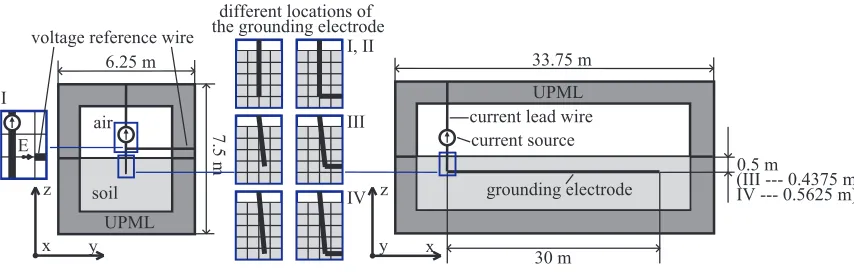
UPML
30 m
0.5 m z
x y air
33.75 m 6.25 m
7.5 m
UPML z
y x
current lead wire voltage reference wire
grounding electrode current source soil
I, II
III
IV E
different locations of the grounding electrode
I
(III --- 0.4375 m, IV --- 0.5625 m)
Figure 5. Calculation model for validation of the modifications. I — model of Railton et al.; II, III, IV — model of Guiffaut et al.
The current form is set by [4]
i(t) =
m
k=1
I0k
ηk
exp
− t τ2k
(t/τ1k)nk
1 + (t/τ1k)nk, ηk
= exp
−τ1k
τ2k
nkτ2k
τ1k
1/nk
, (32)
whereI01= 15.4 kA,I02= 7.2 kA, n1 = 3.4,n2 = 2,τ11= 0.6µs, τ12= 4µs, τ21= 4µs,τ22= 120µs.
The calculation results are shown in Fig. 6 (the simulations are carried not only for the dispersive soil but also for the soil with constant permittivity). It is seen from the figure that FDTD method simulation results are in good agreement with those of the HEM method. The difference between the results of these two methods is approximately the same both for the cases with dispersion and without it, which indicates that the difference is caused by peculiarities of the methods (or models) itself related to the injection of the current into the grounding electrode and calculation of the voltage rather than inaccuracies of the proposed modifications.
0 0.5 1 1.5 2
0 2 4 6 8
Voltage, MV
Time, μs
HEM method Railton et al., I Guiffaut et al., II Guiffaut et al., III Guiffaut et al., IV 0.8
1 1.2
2 4 6
0 1 2 3 4
0 2 4 6 8
Voltage, MV
Time, μs
1 1.5 2
2 4 6
(a) (b)
=4000 m
ε=10, ρ =2000 m
( ), ( )
( ), ( )
Ω
ε ω ρ ω
ε=10, ρ Ω
ε ω ρ ω
Figure 6. GPR of the horizontal electrode simulated by different methods. HEM method simulation results are adopted from [2]. (a)ρ0= 2000 Ω·m, (b) ρ0 = 4000 Ω·m.
6. CONCLUSIONS
The modifications of the thin wire model proposed by Guiffaut et al. and the model proposed by Railton et al. are presented. With the proposed modifications, it is now possible to perform calculations with thin wires located in Debye media in the FDTD method, which is important, for example, for simulations involving wires located in soils with dispersive properties. As long as the modifications are based on the efficient ADE method, their implementation adds a relatively small amount of floating-point operations and storage needed for unknowns to the thin wire models (in the case of the model proposed by Railton et al., only a correction of the coefficients is needed). It is expected that thin wires in other media (such as Lorenz and Drude) can be modeled similarly with the ADE method.
REFERENCES
2. Alipio, R. and S. Visacro, “Frequency dependence of soil parameters: effect on the lightning response of grounding electrodes,” IEEE Trans. Electromagn. Compat., Vol. 55, No. 1, 132–139, 2013.
3. Diaz, L., C. Miry, A. Reineix, C. Guiffaut, and A. Tatematsu, “FDTD transient analysis of grounding grids. A comparison of two different thin wire models,” 2015 IEEE International Symposium on Electromagnetic Compatibility (EMC), 501–506, 2015.
4. De Conti, A. and S. Visacro, “Analytical representation of single- and double-peaked lightning current waveforms,”IEEE Trans. Electromagn. Compat., Vol. 49, No. 2, 448–451, 2007.
5. Visacro, S. and R. Alipio, “Frequency dependence of soil parameters: experimental results, predicting formula and influence on the lightning response of grounding electrodes,” IEEE Trans. Power Delivery, Vol. 27, No. 2, 927–935, 2012.
6. Kelley D. F., T. J. Destan, and R. J. Luebbers, “Debye function expansions of complex permittivity using a hybrid particle swarm-least squares optimization approach,” IEEE Trans. Antennas Propag., Vol. 55, No. 7, 1999–2005, 2007.
7. Okoniewski, M., M. Mrozowski, and M. A. Stuchly, “Simple treatment of multi-term dispersion in FDTD,” IEEE Microw. Guided Wave Lett., Vol. 7, No. 5, 121–123, 1997.
8. Holland, R. and L. Simpson, “Finite-difference analysis of EMP coupling to thin struts and wires,”
IEEE Trans. Electromagn. Compat., Vol. 23, No. 2, 88–97, 1981.
9. Guiffaut, C. and A. Reineix, “Cartesian shift thin wire formalism in the FDTD method with multiwire junctions,”IEEE Trans. Antennas Propag., Vol. 58, No. 8, 2658–2665, 2010.
10. Ledfelt, G., “A stable subcell model for arbitrarily oriented thin wires for the FDTD method,”Int. J. Numer. Model. Electron. Netw. Devices Fields, Vol. 15, No. 5–6, 503–515, 2002.
11. Edelvik, F., “A new technique for accurate and stable modeling of arbitrarily oriented thin wires in the FDTD method,”IEEE Trans. Electromagn. Compat., Vol. 45, No. 2, 416–423, 2003.
12. Guiffaut, C., A. Reineix, and B. Pecqueux, “New oblique thin wire formalism in the FDTD method with multiwire junctions,” IEEE Trans. Antennas Propag., Vol. 60, No. 3, 1458–1466, 2012. 13. Umashankar, K. and A. Taflove, “Calculation and experimental validation of induced currents on
coupled wires in an arbitrary shaped cavity,” IEEE Trans. Antennas Propag., Vol. 35, No. 11, 1248–1257, 1987.
14. M¨akinen, R. M., J. S. Juntunen, and M. A. Kivikoski, “An improved thin-wire model for FDTD,”
IEEE Trans. Microw. Theory Techn., Vol. 50, No. 5, 1245–1255, 2002.
15. Noda, T. and S. Yokoyama, “Thin wire representation in finite difference time domain surge simulation,”IEEE Trans. Power Delivery, Vol. 17, No. 3, 840–847, 2002.
16. Railton, C. J., D. L. Paul, I. J. Craddock, and G. S. Hilton, “The treatment of geometrically small structures in FDTD by the modification of assigned material parameters,”IEEE Trans. Antennas Propag., Vol. 53, No. 12, 4129–4136, 2005.
17. Taniguchi, Y., Y. Baba, N. Nagaoka, and A. Ametani, “An improved thin wire representation for FDTD computations,” IEEE Trans. Antennas Propag., Vol. 56, No. 10, 3248–3252, 2008.
18. Taflove, A. and S. C. Hagness, Computational Electrodynamics: The Finite-Difference Time-Domain Method, 3rd Edition, Artech House, 2005.
![Figure 6. GPR of the horizontal electrode simulated by different methods. HEM method simulationresults are adopted from [2]](https://thumb-us.123doks.com/thumbv2/123dok_us/1984429.1262328/8.612.116.505.250.489/figure-horizontal-electrode-simulated-dierent-methods-simulationresults-adopted.webp)