The Diffraction by the Half-Plane with the Fractional Boundary
Condition
Eldar Veliyev1, 2, *, Vasil Tabatadze1, Kamil Kara¸cuha1, and Ertu˘grul Kara¸cuha1
Abstract—The electromagnetic plane wave diffraction by the half-plane with fractional boundary conditions is considered in this article. The theoretical part is given based on that the near field, pointing vector, and energy density distribution are calculated for different values of the fractional order. The results are compared with classical cases for marginal values of the fractional order. Interesting results are obtained for fractional orders between marginal values. Results are analyzed.
1. INTRODUCTION
The problem investigated in the study is a new approach to the diffraction problem including a half-plane surface and the half-plane wave as an incidence wave. The new method is called as fractional derivative method (FDM). The method explains the continuous intermediate stages of the two canonical states of the electromagnetic field.
In general, the fractionalization of the operators such as derivative, integral, or curl allows extending the usage of the operators. The intermediate stages obtained by the tools of fractional calculus give important results in many branches of science such as diffusion problems, system modelling with friction, and data modelling [1–3]. The first studies related to the fractional approach for the electromagnetic theory and its applications are investigated by Engheta [4–6]. Then, Veliyev et al. developed the idea for the boundary condition which is called the fractional boundary condition (FBC) [7]. The fractional boundary condition used in previous works [8–11] explains a new material property (Perfect Electric Conducting (PEC), Perfect Magnetic Conducting (PMC) or in between). Therefore, by the proposed method, not only the PEC and PMC cases are investigated, but also the cases between two states are studied, and the comparison between the previously studied method and the proposed method is done. The diffraction by half-plane can be assumed to be simplest canonical but intensively investigated structure with the edge [12]. Although the problem for the conducting sheet was solved more than 50 years ago, the problem keeps its importance and is still studied for the non-stationary scenario investigating the effect of the motion on the scattering [13, 14]. Previously, for diffraction by a half-plane with impedance, the perfect electric and magnetic conducting cases were studied not only analytically but also numerically [15–17]. The fundamentally analytical methods for the problem are the Wiener-Hopf and Maliuzhinetz methods. Even though both methods are based on a solid and well-established process, the main disadvantages of these methods are to have lasting and complex mathematical procedures. In [18], a new and practical analytical approach for the plane wave diffraction by a perfectly conducting half-plane is developed for theE and H polarized plane waves. The method uses Laguerre polynomials to expand the induced current on the plane as Method of Moments.
In the following section, the formulation of the problem and the theoretical background are presented. In Section 3, the numerical results are given, and also the comparisons between different methods are done. Then, the conclusion is drawn.
Received 24 October 2019, Accepted 20 December 2019, Scheduled 8 January 2020 * Corresponding author: Eldar Veliyev ([email protected]).
2. THE FORMULATION OF THE PROBLEM
In the formulation of the problem section, the main theoretical background is highlighted. In Figure 1, the geometry of the problem is given.
Figure 1. Geometry of the problem.
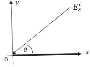
The incidenceE-polarized electromagnetic wave can be denoted asEzi =e−ik(xcosθ+ysinθ)ˆez. Note that the time dependency is e−iωt; θ is the angle of incidence; and ˆez is the unit vector in the z
direction. The incidence wave is scattered by a half-plane located aty= 0, x[0,∞). The total electric
fieldEz=Eiz+Ezs must satisfy the fractional boundary condition given as follows.
DνkyEz(x, y) = 0, y→ ±0, x >0 (1) Here,Dνky denotes the operator of the fractional derivative. The derivative is taken with respect to ky
in the order of fractional order ν, and y is the normal direction to the half-plane. Note that k is the wavenumber (k = 2π/λ); λ is the wavelength of the wave in free space; and ky is the dimensionless parameter. Keep in mind that the derivative is taken by the integral of Riemann-Liouville which has the next form [2]:
−∞Dνx(x) = 1 Γ(1−ν)
d dx
x
−∞
f(t)dt
(x−t)ν,0< ν <1 (2)
Scattered field can be represented by using the fractional Green’s function [7, 8]
Ezs(x, y)≡ ∞
0
f1−νxGν(x−x, y)dx (3)
Here, f1−ν(x) is the unknown fractional current density, andGν is the fractional Green’s function as follows.
Gνx−x, y=−i 4D
ν
kyH0(1)(k
(x−x)2+y2) (4)
whereH0(1) is the Hankel’s function of zero order and first kind.
After substituting Eq. (2) into fractional boundary conditions in Eq. (1), the following equation is achieved. −i 4 D 2ν ky ∞ 0
f1−νxH0(1)
k
(x−x)2+y2
dx =−Dkyν Ezi(x, y), x >0. (5)
In order to solve Eq. (4), the spectral representation of the Hankel function and the Fourier transform of f1−ν are used. The Fourier transform off1−ν is given as follows:
F1−ν(q) = ∞
−∞
˜
f1−ν(ξ)e−ikqξdξ= ∞
0
f1−ν(x)e−ikqxdx,
Then, the scattered electric field is expressed via the Fourier transformF1−ν(q) as given in Eq. (5).
Ezs(x, y) =−ie
±iπν 2
4π
∞
−∞F
1−ν( q)eik
xq+|y|√1−q2
(1−q2)ν−12 dq (6)
Using the Fourier transform and the spectral representation of the Hankel function, Eq. (4) is reduced to the dual integral equation (DIE) with respect to F1−ν(q):
⎧ ⎪ ⎪ ⎪ ⎪ ⎪ ⎪ ⎨ ⎪ ⎪ ⎪ ⎪ ⎪ ⎪ ⎩ ∞ −∞
F1−ν(q)eikξq(1−q2)ν−12dq=−4πeiπ2(1−3ν)sinνθe−ikξcosθ, ξ >0
∞
−∞
F1−ν(q)eikξq= 0, ξ <0
(7)
For the limit cases of the fractional orderν = 0 and ν = 1, these equations are reduced to well-known integral equations used for the PEC and PMC half-planes [20], respectively. The main purpose of the paper is to generalize the solution of the integral equations for any arbitrary fractional order (FO)
ν ∈[0,1].
Note that for the caseν= 0.5, the left part of the first integral equation in Eq. (6) gives the inverse Fourier transform. Then, the fractional current density can be found analytically as follows
f0.5(x) =Ae−ikxcosθ (8)
whereA=−2ke−iπ4sin(θ).
The Fourier transform of Eq. (7) gives F0.5(q) = πkA(δ(q + cos(θ))− π(q+cos(1 θ))). The Fourier transform of the fractional current density can be inserted into Eq. (5), then the scattered electric field becomes as Eq. (8).
Ezs(x, y) =GAπ
k(I1+I2) (9)
whereG=−4iπe±iπ4 and,
I1 = eik(−xcos(θ)+|y|sin(θ))sin−0.5(θ)
I2 = −i π
∞
−∞
eik
qx+|y|√1−q2 q+ cos (θ)
1−q2−14dq
The second integral (I2) in Eq. (8) is evaluated numerically for the results presented in Section 3,
Numerical Results.
For the general case of ν ∈ [0,1], the normalized fractional current density ˜f1−ν is expanded as orthogonal series by Laguerre polynomials with unknown coefficients fnν.
˜
f1−ν
ς
k =e
−ςςν−1 2
∞
n=0
fnνLν−12
n (2ς), ς =kx (10)
Throughout the study, Meixner’s edge conditions need to be taken into account for x→0 as including the weightingςν−12 in Eq. (9) [7]. This representation guarantees that ˜f1−ν satisfies the edge conditions.
Fourier transform of Eq. (9) can be found as given in Eq. (10).
F1−ν(q) = 1
k
∞
n=0
fnνγnν (iq−1) n
(iq+ 1)ν+n+12
(11)
whereγnν = Γ(n+ν+12)
Γ(n+1) . Here, the following property is utilized [19].
∞
0
e−ς(1+iq)ςν−12Lν− 1 2
n (2ς)dς =γnν (iq−1) n
In order to get the system of linear algebraic equations (SLAE) given in Eq. (11), first, Eq. (10) is inserted into the first equation of Eq. (7), then both sides of the integral Equation (7) is multiplied by
e−ςςν−12Lν− 1 2
n (2ς). After that, an integral is taken from 0 to ∞ with respect to ς for Eq. (7) by using the same property mentioned above.
∞
n=0
fnνCnmν =Bmν (12)
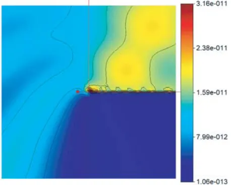
Figure 2. Near Ez field Distribution calculated with our method Fractional at ν= 0.01, θ= π2.
Figure 3. Near Ez field distribution Result obtained with analytical solution at ν = 0.01,
θ= π2.
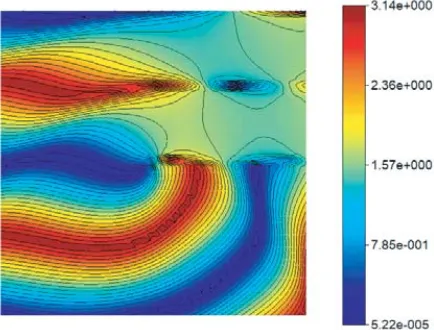
Figure 4. Poynting vector distribution at ν = 0.01,θ= π2.
where,
Cnmν = 1
kγ ν
n(−1)n+m
∞
−∞
(1−iq)n−m−ν−12
(1 +iq)n−m+ν+12
(1−q2)ν−12dq
Bmν = −4πeiπ2(1−3ν)sinν(θ) (icos (θ)−1)
m
(icos (θ) + 1)ν+m+12
After solving this SLAE, unknown coefficients fnν are determined. This gives the ability to find the fractional current density ˜f1−ν with formula (9) and its Fourier transform with formula (10). Then, the near scattered electric field distribution can be found with Eq. (5).
Before ending the theoretical part, it is needed to mention that there exists a relation between the fractional order and impedance value (η) which isη=−siniθtan(π2ν) [9]. Here we mean the impedance of the strip normalized by the impedance of the free space.
Figure 6. Ez Phase distribution obtained with our method at ν= 0.01, θ= π2.
Figure 7. Ez Phase distribution obtained with analytical method at ν= 0.01, θ= π2.
Figure 8. Near Ez field Distribution calculated
with our method Fractional at ν= 1, θ= π2.
Figure 9. Near Ez field distribution Result
3. NUMERICAL RESULTS
Based on the above mentioned mathematical algorithm, the program package was created in MatLab which gives ability to calculate near field distribution, Poynting vector distribution, and energy density distribution. The obtained results and their analysis are given below. For all results obtained with our approach presented below, 70 terms were used in the sum in Eq. (11).
First we considered the case of fractional orderν = 0.01 which is close to the PEC. For this case, there exist the analytical solution given in the book [20].
Figure 2 shows the near field distribution for this case obtained by our approach. Under the half-plane, we see the shadow which is expected. Fig. 3 shows the same scenario calculated with the analytical formula. Deviation from the analytical result is less than 4% as seen on the rulers.
Figure 4 shows the pointing vectors distribution for the same fractional order. As we see, the higher energy flow is on the left to the half-plane. Above the half-plane, the vortices of the electromagnetic energy are observed. Fig. 5 shows the energy density distribution for the same case. If we compare
Figure 10. Poynting vector distribution atν = 1,
θ= π2.
Figure 11. Energy density distribution atν = 1,
θ= π2.
Figure 12. Ez Phase distribution obtained with
our method at ν= 1, θ= π2.
Figure 13. Ez Phase distribution obtained with
this picture to Fig. 4, we see that maximum of the energy density corresponds to the upper side of the half-plane, which means that we have a standing wave. In the left part to the half-plane, we again see energy density but not as intensive as energy flux given in Fig. 4.
Figure 6 shows the phase distribution for this scenario, and energy flows perpendicularly to the phase iso-lines. This result is calculated with our method. Fig. 7 shows the same phase distribution calculated with the analytical formula, and they coincide.
After that we considered case when fractional order is ν = 1. Again we make comparison with analytical results. Fig. 8 gives the near field distribution obtained with our method and Fig. 9 the same distribution obtained with analytical formula. The pictures are very similar.
Again below the half-plane is the shadow, but the structure of the field on the upper part to the half-plane is different from the case ofν = 0.01.
Figure 10 shows the Poynting vector distribution. Again, we have main flux on the left part to the
Figure 14. NearEz field Distribution calculated
with our method Fractional at ν= 1, θ= 34π.
Figure 15. Near Ez field distribution Result
obtained with analytical solution atν = 1,θ= 34π.
Figure 16. NearEz field Distribution calculated with our method Fractional at ν= 0.5,θ= π2.
Figure 17. Near Ez field distribution Result obtained with analytical solution at ν = 0.5,
half-plane. Fig. 11 shows the energy density distribution, and as in the previous case the energy density maximum is above the half-plane.
Figure 12 shows the phase distribution for this scenario obtained with our method, and it is compared to Fig. 13 which is obtained analytically. Deviation from the analytical result is less than 1% as seen on the rulers.
All the cases considered above are for normal incidence. Fig. 14 shows the scenario when the fractional order is again ν = 1, and the incidence angle is θ = 34π. The result is obtained with our method and is compared to Fig. 15 which is obtained analytically. Deviation from the analytical result is less than 10% as seen on the rulers.
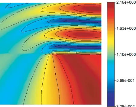
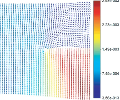
The cases of fractional order ν = 0.01 and ν = 1 correspond to the classical cases which are well known. However, we represent the results here to validate our method. Our method gives ability to consider the case when the classical solution does not exist. If we put ν = 0.5 it gives the material for
Figure 18. Poynting vector distribution at ν = 0.5,θ= π2.
Figure 19. Energy density distribution at ν = 0.5,θ= π2.
Figure 20. NearEz field Distribution calculated
with our method Fractional at ν= 0.75, θ= π2.
Figure 21. Near Ez field Distribution calculated
which the corresponding impedance isη =−i. Such a material does not exist in nature, but it has very interesting properties. If such a material can be made artificially, it will have lot of useful applications. Figure 16 shows the near field distribution whenν = 0.5 as we see that under the half-plane the high field values are observed instead of shadow. This is not an ordinary behavior of the material. It seems that such a material works like a capacitor but for electromagnetic wave. It accumulates the energy and then radiates it below (this is also clearly seen in Figs. 18–19). Such a behavior is known for resonators, but usual resonators need more complex structure. Also antennas have such a behavior when they direct energy in a certain direction. Fig. 17 shows the same result obtained with Equation (8) given in the theoretical part. Deviation from the analytical result is less than 1% as seen on the rulers. Figure 18 shows the Poyntng vector distribution. Here, we see that in reality the energy flow is in the lower part of the half-plane. This proves the idea given in the description of Fig. 16. Fig. 19 shows the energy density distribution, and here also most part of the energy is given in the lower part of the half-plane which is very different from the cases of Figures 4–5 and 10–11.
Figure 20 shows the near field distribution for the fractional order ν = 0.75, and again we have unusual behavior of the material. This is partly similar to the caseν = 1 and partlyν = 0.5 case.
Figure 21 shows the caseν = 0.25 which is partly similar to the caseν = 0.01 and partlyν = 0.5.
4. CONCLUSION
In this article, the plane wave diffraction by the half-plane with fractional boundary conditions is considered. The results for the marginal values of the fractional order are in good agreement with the results obtained by the classical methods. For the values of the fractional order between the marginal values, interesting results are obtained which describe a new type of material with interesting properties. Such a material if it can be created artificially may have wide application in the resonators or antenna devices.
REFERENCES
1. Samko, S. G., A. A. Kilbas, and O. I. Marichev, Fractional Integrals and Derivatives, Theory and Applications, Gordon and Breach Science Publishers, Langhorne, PA, USA, 1993.
2. Onal, N. ¨¨ O., K. Kara¸cuha, G. H. Erdin¸c, B. B. Kara¸cuha, and E. Kara¸cuha, “A mathematical approach with fractional calculus for the modelling of children’s physical development,”
Computational and Mathematical Methods in Medicine, Vol. 2019, Article ID 3081264, 13 pages, 2019, https://doi.org/10.1155/2019/3081264.
3. Axtell, M. and M. E. Bise, “Fractional calculus application in control systems,” Proceedings of the IEEE 1990 National Aerospace and Electronics Conference (NAECON 1990), Pittsburgh, PA, USA, June 1990.
4. Engheta, N., “Use of fractional integration to propose some “fractional” solutions for the scalar Helmholtz Equation,”Progress In Electromagnetics Research, Vol. 12, 107–132, 1996.
5. Engheta, N., “Fractional curl operator in electromagnetics,” Microwave and Optical Technology Letters, Vol. 17, No. 2, 86–91, 1998.
6. Engheta, N., “Phase and amplitude of fractional-order intermediate wave,”Microwave and Optical Technology Letters, Vol. 21, No. 5, 338–343, 1999.
7. Veliev, E. I., T. M. Ahmedov, and M. V. Ivakhnychenko, “Fractional operators approach and fractional boundary conditions,” Electromagnetic Waves, 28, Zhurbenko V. (editor), IntechOpen, Rijeka, Croatia, 2011, doi: 10.5772/16300.
8. Veliev, E. I., M. V. Ivakhnychenko, and T. M. Ahmedov, “Fractional boundary conditions in plane waves diffraction on a strip,” Progress In Electromagnetics Research, Vol. 79, 443–462, 2008. 9. Ivakhnychenko, M. V., E. I. Veliev, and T. M. Ahmedov, “Scattering properties of the strip
10. Tabatadze, V., K. Kara¸cuha, and E. I. Veliev, “The fractional derivative approach for the diffraction problems: plane wave diffraction by two strips with the fractional boundary conditions,”Progress In Electromagnetics Research, Vol. 95, 251–264, 2019.
11. Kara¸cuha, K., E. I. Veliyev, V. Tabatadze, and E. Kara¸cuha, “Analysis of current distributions and radar cross sections of line source scattering from impedance strip by fractional derivative method,”
Advanced Electromagnetics, Vol. 8, No. 2, 108–113, 2019.
12. Bowman, J. J., T. B. Senior, and P. L. Uslenghi,Electromagnetic and Acoustic Scattering by Simple Shapes (Revised Edition), 747 p., Hemisphere Publishing Corp., New York, No individual items are abstracted in this volume, 1987.
13. Idemen, M. and A. Alkumru, “Relativistic scattering of a plane-wave by a uniformly moving half-plane,”IEEE Transactions on Antennas and Propagation, Vol. 54, No. 11, 3429–3440, 2006. 14. Da Rosa, G. S., J. L. Nicolini, and F. J. V. Hasselmann, “Relativistic aspects of plane wave
scattering by a perfectly conducting half-plane with uniform velocity along an arbitrary direction,”
IEEE Transactions on Antennas and Propagation, Vol. 65, No. 9, 4759–4767, 2017.
15. Carlson, J. F. and A. E. Heins, “The reflection of an electromagnetic plane wave by an infinite set of plates,” Quart. Appl. Math., Vol. 4, 313–329, 1947.
16. Senior, T. B. A., “Diffraction by a semi-infinite metallic sheet,”Proc. Roy. Soc. London, Seria A, Vol. 213, 436–458, 1952.
17. Senior, T. B. A., “Diffraction by an imperfectly conducting half plane at oblique incidence,”Appl. Sci. Res., Vol. B8, 35–61, 1959.
18. Veliev, E. I., “Plane wave diffraction by a half-plane: A new analytical approach,” Journal of Electromagnetic Waves and Applications, Vol. 13, No. 10, 1439–1453, 1999.
19. Prudnikov, H. P., Y. H. Brychkov, and O. I. Marichev, Special Functions, Integrals and Series, Vol. 2, Gordon and Breach Science Publishers, 1986.