Feature Encoding Strategies for Multi-View Image Classification

(1)

Western University Western University

Scholarship@Western

Electronic Thesis and Dissertation Repository

1-26-2016 12:00 AM

Feature Encoding Strategies for Multi-View Image Classification

Kyle Doerr

The University of Western Ontario

Supervisor

Jagath Samarabandu

The University of Western Ontario

Graduate Program in Electrical and Computer Engineering

A thesis submitted in partial fulfillment of the requirements for the degree in Master of Engineering Science

Follow this and additional works at: https://ir.lib.uwo.ca/etd

Part of the Artificial Intelligence and Robotics Commons, and the Software Engineering Commons

Recommended Citation Recommended Citation

Doerr, Kyle, "Feature Encoding Strategies for Multi-View Image Classification" (2016). Electronic Thesis and Dissertation Repository. 3500.

https://ir.lib.uwo.ca/etd/3500

This Dissertation/Thesis is brought to you for free and open access by Scholarship@Western. It has been accepted for inclusion in Electronic Thesis and Dissertation Repository by an authorized administrator of

(2)

Machine vision systems can vary greatly in size and complexity depending on the task at hand. However, the purpose of inspection, quality and reliability remains the same. This work sets out to bridge the gap between traditional machine vision and computer vision. By applying powerful computer vision techniques, we are able to achieve more robust solutions in manufacturing settings. This thesis presents a framework for applying powerful new image classification techniques used for image retrieval in the Bag of Words (BoW) framework. In addition, an exhaustive evaluation of commonly used feature pooling approaches is conducted with results showing that spatial augmentation can outperform mean and max descriptor pool-ing on an in-house dataset and the CalTech 3D dataset. The results of the experiments contained within, details a framework that performs classification using multiple view points. The results show that the feature encoding method known as Triangulation Embedding outperforms the Vector of Locally Aggregated Descriptors (VLAD) and the standard BoW framework with an accuracy of 99.28%. This improvement is also seen on the public Caltech 3D dataset where the improvement over VLAD and BoW was 5.64% and 12.23% respectively. This proposed multiple view classification system is also robust enough to handle the real world problem of camera failure and still classify with a high reliability. A missing camera input was simulated and showed that using the Triangulation Embedding method, the system could perform classifi-cation with a minor reduction in accuracy at 98.89%, compared to the BoW baseline at 96.60% using the same techniques. The presented solution tackles the traditional machine vision prob-lem of object identification and also allows for the training of a machine vision system that can be done without any expert level knowledge.

Keywords: Machine Vision, Manufacturing reliability, Triangulation embedding, Multi-view image classification, Multiple Multi-view vision system

(3)

Acknowledgements

I would first like to thank my supervisor, Dr. Samarabandu. I have been his student for several years now, and he has been such a positive influence during my time at Western. His patience, expertise and his open-mindedness have made this possible. His willingness to take a chance on me and help foster my education is something I will forever cherish. Thank you Professor.

Next I would like to thank Dr. Wang. He has been friendly and willing to cater to my educational needs. He welcomed me into his research lab to an amazing group of people who have become dear friends to me.

I want to thank the industry sponsor that supported this work, Sightline Innovation Inc. Specifically Wallace (Wally) Trenholm, Maithili Mavinkurve and Mark Alexiuk. Their vision-ary leadership and expertise have been crucial in solving industrial problems using machine learning.

I would like to thank my parents. Their hard work and belief in the importance of education has provided me with this opportunity. I would not have made it this far without their support. I would also like to my dear friends I have met during my time at Western. Through all of our years together we have watched each other grow. In no particular order, I would like to thank - Paria, Chris Line and S., Fuad, Tania, Guy, Veronik, Ken, Matt, Ashley, Justine, Jeremy and Colin. Thank you.

(4)

(5)

4.6 Classification performance on in-house dataset using the BoW model compar-ing SIFT, SURF and ORB features against vocabulary size uscompar-ing a scompar-ingle view 52 4.7 Classification performance on CalTech dataset using the BoW model with vary-ing vocabulary size usvary-ing a svary-ingle view . . . 53

4.8 Classification performance showing the impacts of using different combina-tions of views and dictionary size on in-house dataset . . . 54

4.9 Classification performance using multiple views of the CalTech 3D dataset . . 56

4.10 Confusion matrix of the CalTech 3D dataset single view with classification results averaged over 10-folds . . . 57

(10)

4.12 A comparison on using different methods of utilizing the visual vocabulary for

image classification using in-house dataset . . . 59

4.13 Heat Map of Grid Search for polynomial degree 2 parameters . . . 62

4.14 Heat Map of Grid Search for polynomial degree 3 parameters . . . 63

4.15 Heat Map of Grid Search for RBF kernel . . . 64

4.16 Generating spatial pyramids [32] . . . 65

4.17 An example of spatial histograms . . . 68

4.18 Spatial histograms and feature pooling applied to in-house dataset . . . 71

4.19 Spatial histograms and feature pooling applied to CalTech 3D dataset . . . 72

4.20 Classification improvements when adding spatial histograms . . . 73

4.21 The results of the in-house dataset using the VLAD encoding approach . . . 74

4.22 Classification of Caltech using the VLAD encoding approach . . . 75

4.23 In-House eigenvalue distribution of PCs on feature vectors using VLAD en-codings . . . 76

4.24 CalTech eigenvalue distribution of PCs on feature vectors using VLAD . . . . 77

4.25 Similarity scores histogram of Shoe vs. Iron classes using BoW . . . 79

4.26 Similarity score histogram of Shoe vs. Iron classes using Triangulation Em-bedding . . . 79

(11)

List of Tables

4.1 Comparison of classification time [11] . . . 55 4.2 Hyper-parameter search for several kernels and the affects on classification . . . 62 4.3 Comparison of the Histogram Intersection andX2kernels . . . 67 4.4 Effects of Dimensionality Reduction when using VLAD encodings . . . 76 4.5 Comparison of the Triangulation Embedding method on the in-house dataset . 78 4.6 Comparison of the Triangulation Embedding method on the CalTech 3D set . . 78 4.7 Comparison of the Triangulation Embedding method on the in-house dataset . 80 4.8 Comparison of the Triangulation Embedding method on the CalTech dataset . 81 4.9 Comparison of the feature encoding rates . . . 81

(12)

BoW Bag of Words

BRIEF Binary Robust Independent Elementary Features FAST Features from Accelerated Segment Test

HIK Histogram Intersection Kernel ORB Oriented FAST and Rotated BRIEF PCA Principal Component Analysis PMK Pyramid Match Kernel

SIFT Scale-Invariant Feature Transform SURF Speeded-Up Robust Features SVD Singular Value Decomposition SVM Support Vector Machine

VLAD Vector of Locally Aggregated Descriptors

(13)

Chapter 1 Introduction

1.1 Motivation

Machine vision is the process of applying image processing and analysis to automate certain tasks. This term is typically applied to automating lower level tasks such as the reading of optical characters, defect inspection, and object counting. Computer vision on the other hand focuses on higher level tasks such as object and person classification, detection, tracking and segmentation. Typically, computer vision tasks use more complex methods and models for representing visual data. Often at that core of computer vision, these tasks are more difficult than machine vision because of variability in the input data and often the data comes from images that the input is not from a controlled environment. Trying to get a computer to interpret and make decisions given a wide variety of complex visual information like a human would is more challenging when the image or video is captured by a human and can contain variable poses and possible occlusions. This would not be the case for machine vision environments in which the camera is often in a fixed position and some knowledge of what to expect in the image would be known beforehand.

Machine vision will often use more low level techniques that have proven themselves to be useful in industrial settings but unable to handle the large variations in input data. Machine vision often requires a clear specified problem that can only be handled in a controlled environ-ment resulting in input data that has less variance. For a product that uses machine vision for object verification and defect detection to have any use in an industrial setting it must provide

(14)

very high accuracy and always be more reliable and faster than human inspection. Depending on the application in computer vision detecting object defects can have a wide variability in accuracy depending on the application and technique used. For example, a system that can achieve a 5% misclassification rate may achieve state of the art results for a particular learn-ing task and that may be acceptable, but in an industrial settlearn-ing that can potentially process thousands of parts a day as say defective, this system may no longer be acceptable at fully automating a task.

Machine vision systems offer high accuracy, but are limited to their environment and often require very careful parameter tuning. Computer vision on the other hand has more freedom in the variability of the data and while often has parameters tuning, typically it is not as stringent with the parameter learning being treated sometimes as a learning task in itself; say using a validation set. Our problem that we try to answer is, if machine vision works well on easier, more well defined problems but not on challenging problems with greater variability in the input and computer vision techniques perform reasonably well on more challenging hard prob-lems, is there a way to bridge the gap between the two and use the strengths of computer vision approaches in industrial applications?

In many manufacturing settings assembly lines use conveyor belts to move parts to different stages of production. In places that manufacture auto parts the products might have minimal variations in size, orientation, texture and luster. This is because each class of part is specific to the location of the car it is on and the part design between car models and the year of manufacture often varies. Many manufacturers employ people to manually inspect these parts but given the level of similarity among the parts moving on a belt the current approach is prone to human error. Correct part classification is essential for quality control and has financial implications for automotive manufacturers when high standards are not met. In this work we propose a low cost framework to address this problem of similar auto part classification using techniques from computer vision.

(15)

1.2. SIFT, SURF,andORBfeatures 3

parts come in different combinations of shapes, sizes and orientations we opted to use multiple cameras angled downwards so that differences among similar parts could be visually captured. More information on these parts can be found in Chapter 3.

1.1.1 Problem Statement

At the time of research, these automotive parts were previously categorized by humans during the manufacturing process. Since there are several stages during the production process, the parts could undergo chemical baths and painting as intermediate processes. Because of these stages, appending simple labels for identification in the form of barcodes is not possible. Using humans to visually categorize these parts and then sort them, resulted in frequent mislabelling that created confusion for the manufacturers during the assembly stage.

Figure 1.1: Images of window pillars, guides1and their location on a vehicle

1.2 SIFT, SURF, and ORB features

1.2.1 SIFT features

Scale-Invariant Feature Transform (SIFT)[34], Speeded-Up Robust Features (SURF)[1], and Oriented FAST and Rotated BRIEF (ORB)[43] are all methods for generating a collection of local image features. These local image features are designed to be invariant to translation, scaling and rotation. In other words, these local features can be reliably matched to a new set of image features, even if the new image has undergone one or all of these transformations.

(16)

The SIFT algorithm has been one of the most popular and widely used algorithms for detecting and describing image features over the past 15 years. The input image is repeatedly blurred and downsampled to create a pyramid. The differences between successive layers in the pyramid is computed to form a subsequent pyramid known as a Difference of Gaussian (DoG) pyramid. Local extrema at both the space neighbourhood and scale neighbourhood of are marked as keypoints.

The keypoints correspond to an edge or a corner. Keypoints that lie on corners are more desirable as they are more discriminative as explained in Section 2.4. The principal curvatures of the keypoint are encoded by the Hessian matrix:

H=

         

Dxx Dxy

Dxy Dyy

         

(1.1)

The ratio of the two eigenvalues of the Hessian matrix gives insight as to whether the keypoint resembles more like a corner or edge. The keypoints that are too similar to edges are removed.

The step after rejecting keypoints is to make the local feature rotationally invariant. Around each keypoint, a histogram containing weighted orientations of local gradients within a circular grid is computed. The dominant gradient becomes the canonical orientation in which the patch is rotated respectively as seen in Figure 1.2b

(a) Difference of Gaussian Pyramid2 (b) SIFT Descriptors from keypoints3 Figure 1.2: Generation of SIFT Descriptors with scale and rotation invariance

2_http:_//_aishack.in_/_tutorials_/_{sift-scale-invariant-feature-transform-log-approximation}

(17)

1.2. SIFT, SURF,andORBfeatures 5

1.2.2 SURF features

The SURF algorithm, like SIFT was based on the same principals of generating local image features that are invariant to translation, scaling and rotation. While SIFT features are quite robust, they are also slow to compute because of some computationally intensive tasks such as repeatedly performing convolution with the Gaussian kernel then downsampling to build the DoG pyramid. SURF uses a different approach to detect keypoints by using a Hessian based detector with the Laplace of Gaussian (LoG) approximation, given by:

H(x, σ)=

         

Lxx(x, σ) Lxy(x, σ) Lxy(x, σ) Lyy(x, σ)

          (1.2)

The SURF approach is then to approximate the LoG using box filters. SIFT has a scale space representation by repeatedly performing blurring and subsampling the input image then computing the DoG pyramid. SURF achieves scale invariance by increasing the box filter size at each level of the pyramid. Using the integral image representation initially introduced by Viola and Jones [48], convolution with a box filter can be performed in constant time O(1) regardless of the filter size.

The determinant of Hessiandet(H) is computed with non-maximum suppression over the space and neighbouring scales. The resulting maxima that are left are identified as keypoints.

The Haar like filters similar to the scale representation step are used to compute the dom-inant gradient in the x & y direction in a circular region. The feature descriptor is built using 4x4 square subregions over the interest point. Gradient and magnitude information are used to build a 64 dimensional feature vector.

1.2.3 ORB features

(18)

(a) Box filters used in feature detection4

(b) Scale-space representation, computed in con-stant time5

Figure 1.3: The shrinking of the hull by erosion

devices with limited memory.

1.3 Thesis Contribution

The contributions of this thesis are as follows:

• A comparison of faster, more efficient computer vision features for the purpose of machine vision are evaluated and compared to traditional feature types and the pros and cons of both are evaluated. The results obtained show that binary ORB features are more suitable than SIFT and SURF features for machine vision applications in controlled environments.

• A demonstration that using more advanced feature encoding techniques that contain higher order information, for the purpose of fine-grained image classification with multiple views has an improved classification accuracy for a machine vision dataset. These results also generalize to the publicly available CalTech 3D dataset.

• A new object classification framework using binary ORB features that can classify very similar automotive parts real-time and provide a meaningful, robust solution for

(19)

1.4. Organization of thesis 7

manufacturing settings.

• A multi view machine vision system that is robust enough that it can handle missing views with a minimal decrease in classification performance. These benefits are

demonstrated in the experimental results and show that the multiple view approach can still provide a robust solution despite camera failure.

1.4 Organization of thesis

This thesis is organized as follows:

• Chapter Two: The challenges associated with computer vision are discussed along with a literature review. Later in the chapter a review about one of the most popular image classification and retrieval techniques and its advancements in the past few years. A brief overview of the machine learning techniques used are also discussed and how they can be used for vision systems.

• Chapter Three: This chapter talks specifically about the engineering problem we set out to solve. The chapter then discusses the physical prototyping environment we used to mimic a real world vision system. We also mention the image preprocessing techniques we used prior to classifying the images. We finally discuss the improvement to the vision system by including multiple views.

• Chapter Four: There is discussion in this chapter about the in-house dataset that we created. We also discuss the use of a publicly available multi view dataset. We then provide a series of classification experiments on both datasets. We provide an assessment on using multiple views in a vision system and various classification techniques. Experimental works and results are presented along with a discussion of results.

(20)

1.5 Experiment Summary

All of the experiments conducted were evaluated on an in-house dataset containing automotive parts as introduced in Section 4.1.1 and the publicly available CalTech 3D dataset presented in Section 4.1.2.

The first set of experiments in Section 4.2.1:Classification Performance with a Single View, evaluated image classification accuracy by the use of single view images of objects within the Bag of Words (BoW) pipeline. These experiments set the baseline for classification accuracy and are compared against further experiments. The results on the first set of experiments show that for single view image classification, accuracy is generally proportional to dictionary size. This can be seen on the in-house dataset in Figure 4.6 and also on the CalTech dataset in Figure 4.7. The figures show that classification accuracy received a boost in performance for larger dictionary sizes. These two experiments also compared a newer binary descriptor against the traditional SIFT descriptor.

The next section of experiments in Section 4.3: Classification Performance with Multiple Views, goes from image classification using a single view to using multiple views on the in-house dataset. The motivation of this experiment was to determine if adding additional views would improve classification performance enough to justify adding more cameras in the frame-work. First, an evaluation of various view points was performed, with the results presented in Figure 4.8. The results show that using the four view points had a substantial increase in clas-sification accuracy. Another trend that was observed, was that increasing the dictionary size improved performance to 95.62% (C=256), much like the case of using a single view. This is the first time to our knowledge that binary features have been applied to multi view image classification within the standard BoW pipeline. In both the single and multiple view experi-ments using ORB features resulted in a higher classification accuracy when compared to SIFT or SURF features.

(21)

1.5. ExperimentSummary 9

finding from this experiment was that using SIFT features resulted in a higher classification performance compared to ORB features on the CalTech dataset for single and multi view clas-sification tasks, this was not the case on the in-house dataset. One of the major differences be-tween the two datasets, is that the CalTech set had large changes in height and scale, whereas the in-house dataset, the cameras were stationary. It is known that ORB features are fast to compute when compared to SIFT as seen in Table 4.1, but SIFT performs better at matching features at different heights and scales. These results reveal that ORB features, in addition to being much faster to compute, can outperform competing techniques when there are not large changes in height and scale, which for this type of industrial vision system would often be the case.

Using ORB features as the baseline, there were significant improvements in classification performance extending from 1 to 8 views as seen in the confusion matrices shown in Figure 4.10 and Figure 4.11 that led to a mean classification accuracy improvement over the 8 object classes by 9.03%. We were able to show that ORB features are ideal when working with datasets more common in machine vision. This is something that limited prior research has been done, comparing traditional features with binary features beyond the traditional feature matching tasks.

(22)

From the previous experiments we had established the multiple view BoW framework per-forming classification with a Support Vector Machine (SVM). Classification using a SVM is a powerful tool and is often considered one of the first options when choosing a classifier. The next set of experiments in Section 4.5.1: Kernel Selection for SVM optimization, was to op-timize the classifier by studying various kernels. The goal was to see if the data was linearly separable and to what degree. If it is not, then using kernels would increase the likelihood of separability in a higher dimensional space. The results presented in Table 4.2 show that the Gaussian kernel could actually perform the best with an accuracy rate of 97.8%. The more recent similarity functions known as the Histogram Intersection and theX2which are also func-tions, were also introduced in Section 4.5.3. The results from these two kernels as presented in Table 4.3 show a considerable increase in classification accuracy of 98.37% and 98.43%. Using the linear kernel as a classification baseline which obtained an accuracy of 95.62%, both of these kernels performed better. In fact, they even performed slightly better then the powerful Gaussian Kernel. It was demonstrated in this section that despite the elegant theory behind ker-nel methods, that the best performing kerker-nel for a multiple view classification problem turned out to be theX2_{additive kernel. This kernel has two key advantages: it is fast to compute and} unlike the traditional SVM kernels there are no hyper parameters that have to be determined thus making it ideal for smaller datasets.

The loss of spatial information that occurs within the BoW framework was addressed using feature pooling techniques is presented in Section 4.6.2. Spatial augmentation and pooling, using: max mean and sum pooling was evaluated and compared to the BoW baseline. The results on both datasets are shown in Figure 4.18 and Figure 4.19. On both datasets using spatial augmentation was the best and outperformed the BoW baseline with an accuracy of 96.08% on the in-house dataset and 93.03 % on the CalTech dataset using the basic linear kernel. The contributions to this experiment is an empirical evaluation of feature pooling and spatial binning techniques applied to a multiple view classification problem.

(23)

1.5. ExperimentSummary 11

shown in Figure 4.21 and gave a classification accuracy of 98.76% and the CalTech dataset in Figure 4.22 with 88.74%. Both of the results reveal a considerable improvement over the standard BoW baseline. Despite the popularity of VLAD feature encodings, very little work until now has been done to see how well this method works when using multiple views and very limited research has been performed to see how well this technique works outside of the traditional single view classification and retrieval problem.

The final encoding strategy evaluated is presented in Section 2.7: Triangulation Embed-ding. Triangulation Embedding maintains the BoW pipeline, yet on several occasions has given state of the art results for the task of image retrieval. Very little research is available on using this technique outside of the image search domain. Using the in-house dataset, the results of this embedding method can be seen in Table 4.5, which gave the best accuracy over all the other techniques at 99.28%. This considerable increase in classification accuracy also general-ized to the CalTech dataset, where the results are presented in Table 4.6, showing an accuracy of 94.38%. There are several contributions contained within this section. Firstly, to the best of our knowledge, Triangulation Embedding has never be applied to a multiple view classification task. The next contribution is we have demonstrated that this powerful method is compatible with binary features, which has the added benefit of being very fast to compute. Thirdly, we were able to demonstrate this powerful technique can be used outside of the computer vision domain and can be used reliably for industrial machine vision applications. By doing this, we have demonstrated a way to help bridge the gap between the two fields of computer vision and machine vision, something this thesis set out to do.

(24)

(25)

Chapter 2 Background and Literature Review

2.1 Machine Learning

Machine learning is a central topic in artificial intelligence and its definition is to have a ma-chine learn from experience of a given task if a given performance measure can be improved from prior experiences [36]. The goal of learning is achieved using concepts from computer science, mathematics and statistics.

There are three main branches in machine learning: reinforcement, unsupervised and su-pervised learning. Reinforcement learning is when an agent is not told what action to take but learns from the feedback it receives after taking an action. At a high level it can be said that the agent attempts to maximize its rewards after making decisions. Unsupervised learning fo-cuses on finding some structure using unlabelled data. The focus of this work is on supervised learning. In which a learning algorithm is given some labelled input and output data and must recognize a pattern and create a mapping function between the input and output [44]. Among all three learning approaches there is a tremendous amount of applications including image and text classification, medical diagnostics, speech recognition and data mining to name a few.

2.2 Image Processing, Understanding and Computer Vision

Digital image processing as defined by [16] is the activity of processing digital images using a digital computer. Image processing is the field of taking an image and applying algorithms

(26)

on the image to return an altered image with some desirable characteristics. Some examples could be performing image enhancement, compression, noise reduction and feature detection to name a few.

Image understanding tries to make sense of what is contained within the image. Image understanding is often seen as a mid-level process that relies on the output of a processed image and is more towards artificial intelligence. Examples of image understanding would be the task of image classification or segmenting an image and labelling the regions.

Computer vision on the other-hand is the closest towards artificial intelligence. The objec-tive being seeing as humans do and having the ability to learn, and make decisions from visual information. An example would be what semantic information can be applied to a series of recognizable objects in an image. While Gonzalez and Woods [16] admits that there is no universally clear definition to distinguish between the three areas they are often thought of as low, mid, and high level processing. The work in this thesis primarily focuses on mid-level processing.

2.2.1 Image Representation

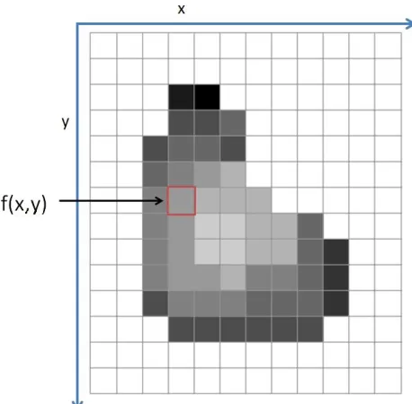
Following the definition of a digital image by Gonzalez and Woods [16], they define a gray scale image as a two dimensional function f(x,y). The values of f are discrete quantities representing the gray scale intensity and x,ycorresponding to a spatial location on the image as seen in Figure 2.1. The standard colour image is a vector valued function consisting of three channels: red, green and blue. Each channel holds the intensity of the colour at that particular pixel and when combined forms a colour image.

2.3 Feature Extraction

(27)

2.4. ORB Features 15

Figure 2.1: A representation of a digital image

point. There are numerous ways to describe these interest points such as colour, orientation, or intensity to name a few. These are referred to as feature descriptors.

2.4 ORB Features

As mentioned earlier the task of feature extraction is two step: detection and description. The most common feature type in computer vision is Scale-Invariant Feature Transform (SIFT) features. SIFT features, developed by David Lowe [34] have many good properties such as scale invariance, but SIFT descriptors are costly to compute. A new trend in the development of feature types that have emerged are known as binary image descriptors because they are faster to compute and match and have smaller memory requirements making them suitable for embedded devices. Rublee et al. [43] developed a method called ORB (Oriented FAST and Rotated BRIEF). The interest point detector uses the FAST (Features from Accelerated Segment Test) method [42] and a modified version of BRIEF as the feature descriptor [4].

(28)

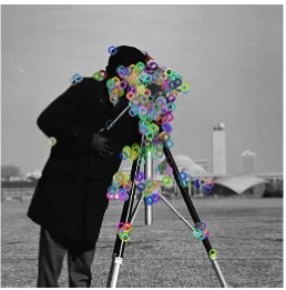
Figure 2.2: ORB features found in an image

the candidate pixelIp, if thenconnected pixels are greater or less than a given thresholdtthe point can be classified as a potential corner. This method exploits the contiguous constraint on the pixel regions to speed up performance by only performing the intensity difference test at the compass directions, thereby avoiding needless computations, if the pixel does not meet the corner criteria as can be seen in Figure 2.3.

The FAST keypoint detector can also identify keypoints that lie along edges in addition to corners. Intuitively, corners have gradients in all directions, whereas an edge will have minimal gradients along the edge direction. It is worth pointing out that having gradients that vary in all directions is a desirable property because it causes the feature to have more variance. This leads to more discriminative features because that feature will respond differently and have a greater response to varying inputs. This can be seen in Figure2.4

(29)

Figure 2.3: A visual of the FAST corner test

Figure 2.4: Keypoints on edges will have little change along the direction of the edge. Gradi-ents along the corner will have a large change in all directions.1

Ex,y =

X

u,v

wu,v(f(u+x,v+y)− f(u,v))2 (2.1)

WhereW [0,1] is the window function that is set to 1 for overlap and 0 otherwise. Using the first order Taylor expansion to approximate a function, let ∇fx and ∇fy be the partial derivatives in the x-direction and y-direction, then:

f(u+x,v+y)≈ f(u,v)+x∇fx+y∇fy (2.2)

(30)

Substituting equation 2.2 into equation 2.1 then:

Ex,y ≈

X

u,v

wu,v(x∇fx+y∇fy)2 (2.3)

Because neighbouring pixels inside the circle may also meet the criteria for being a corner, the authors of ORB use the Harris corner measure [19] to rank the corners. Using 2.3 in matrix form:

Ex,y ≈ (x,y)A

          x y           (2.4)

Where Aknown as the Harris Matrix which is the covariance matrix of the partial deriva-tives of the windowed region defined as:

A=

X

u,v wu,v

         

∇f2

x ∇fx∇fy

∇fx∇fy ∇fy2

          (2.5)

As mentioned earlier corners have gradients that vary in all directions for minor shifts whereas edges are relatively flat along the direction of the edge. The eigenvalues λ1 and λ2 of A capture the amount of covariance. If λ1 > λ2 would mean that most of the gradient is captured in one direction. If λ1 ≈ λ2 then the gradient variance is spread along both the x and y axes which follows the definition above that a corner has gradients in all directions for small shifts whereas an edge only has strong gradients on the orthogonal axis against the edge direction - rather most of the gradients can be captured along one axis. The corner response is efficiently calculated based on these two eigenvalues.

(31)

stored and the desired number of keypoints, now ranked are selected.

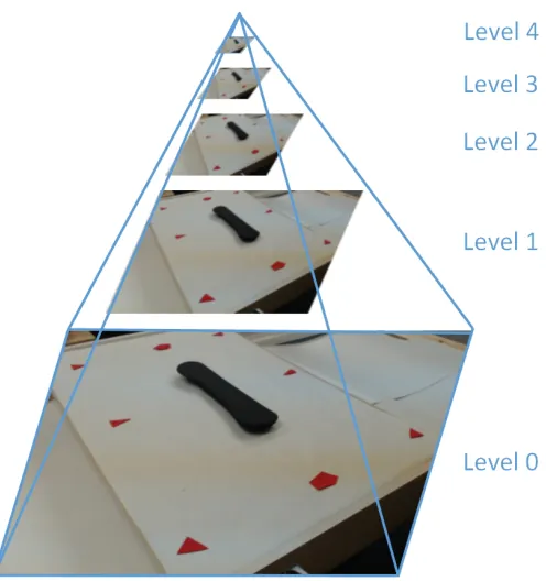
Figure 2.5: Features are produced at each level of the pyramid

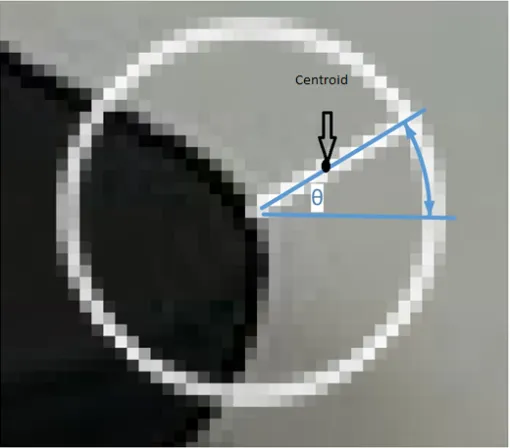
Keypoints are commonly described by their orientation. In the case of corner based interest points, they can be thought of as what angle that corner points to. The FAST method alone does not provide this orientation information, but rather computed by calculating the intensity centroid as proposed by Rosin [41]. In this method the moment of an image patch is defined as:

mpq=

X

x,y

xpyqI(x,y) (2.6)

The centroid locationC(x,y) can then be computed by:

C = m10 m00

,m01 m00

!

(2.7)

By constructing a simple vector from the corner to the centroid the angleθcan be computed as:

(32)

Figure 2.6: A sample showing where the centroid is located within an image

Following this approach the authors of ORB offer a modified version of the BRIEF feature descriptor [4]. The feature descriptor is a bit string on a smoothed image patchp. The bit string is formed by constructing a series of binary testsτdefined by:

τ(p;x,y)=

            

1 :p(x) < p(y)

0 :p(x) ≥ p(y)

(2.9)

The test results are defined by intensity of point p atx. The final descriptor then is built using:

fn(p) := X 1≤i≤n

2i−1τ(p; xi, yi) (2.10)

(33)

2.5. Bag ofWords 21

orientation of the computed intensity centroid. This is done by taking a selection ofnbinary tests at location (xi,yi) defining a 2 xnmatrix:

S= x1, ...,xn y1, ...,yn

!

(2.11)

A rotation matrix inR2is created from the patch orientationθ. The orientation is discretized

by 2π

30 increments. The rotation matrix is defined as:

Rθ =

         

cosθ −sinθ

sinθ cosθ

          (2.12)

The rotation matrix is used to rotate the location of the binary patch tests in 2.10. The series of binary tests is now:

Sθ = RθS (2.13)

The rotated BRIEF operator is then defined as:

gn(p, θ) := fn(p)|(xi,yi) Sθ (2.14)

2.5 Bag of Words

2.5.1 Descriptor Quantization

Descriptor quantization is common among all BoW and extended BoW models. This process is often done through clustering a set of feature descriptors to form what is known as thevisual words. All the visual words or clusters are known as thevisual vocabulary. The most popular clustering algorithm is known ask-meanswhich was first proposed by James MacQueen [35]. One of the earliest mentions of constructing the visual vocabulary using the k-means approach for object categorization is given by Csurka et al.[9]. A set of n feature descriptors can be described as: x1, ...,xnRD. In building the visual vocabulary the descriptor space is partitioned

(34)

has a data to means assignments: q1, ...,qn {1, ...,K}. The centroids are found using the objective function, effectively minimizing thel2_error:

qki= argmin k

kxi−µkk2 (2.15)

Unfortunately with this method the quantization of words is done by vector quantization (or hard quantization) there is no obvious choice for the number of visual words (centroids) and often needs to be determined empirically.

Figure 2.7: k-means data clustering by use of a Voronoi diagram [37]

2.5.2 Histogram Encodings

(35)

2.5. Bag ofWords 23

vocabulary as a preprocessing step. Afterwards on each new query or training image recompute the image descriptorsxXthen assign each descriptor to a visual word by Equation 2.15. The resulting query image is then represented as a 1×nvector withnbeing the number of centroids learned by k-means. This histogram representation is a type of feature vector which can then be used for retrieval or image classification purposes.

Figure 2.8: The process of descriptor encoding

2.5.3 Spatial Pyramids and Pooling

One of the limitations of the BoW model is that it is an orderless representation of encoded keypoints found on a digital image. The geometric and spatial information can reveal a lot about the scene especially when it comes to image classification. This information is lost. One method for overcoming this proposed by Lazebnik et al. [32] is to partition the image into increasing fine sub-regions and computing a histogram per region. This work was adapted from Grauman and Darrell [18] in which the authors proposed thepyramid match kernel(PMK). The PMK is a function that can compare histograms of image descriptors at increasingly coarser grids as seen in Figure 2.9. Each successive level in the pyramid has an increased weight applied to the histogramIldefined as:

Il = 1

(36)

a point and then starts to decrease. There are also variations in the construction of the spatial grids ofmxmbutmxn.

Conversely a more simple approach to incorporate weak geometry is to simply concatenate all the histograms derived from each spatial region. The one obvious problem is that simple concatenation of each histogram per spatial region causes the feature vector to become quite large. One way to circumvent this is to perform sum, max or average pooling. In which each bin of the histogram per level of the pyramid is aggregated by the sum, max or average response.

Figure 2.9: Spatial Pyramid construction on images

Choosing the number of levels in the pyramid or the partition layout remains an open ques-tion and is often found on a validaques-tion set. One thing to keep in mind is that classificaques-tion performance will plateau then start to decrease as the number of grids grows simply because there will be fewer descriptors found in each cell. This will start to cause sparsity in the feature vector and corrupt the image similarity metric.

2.5.4 Support Vector Machines

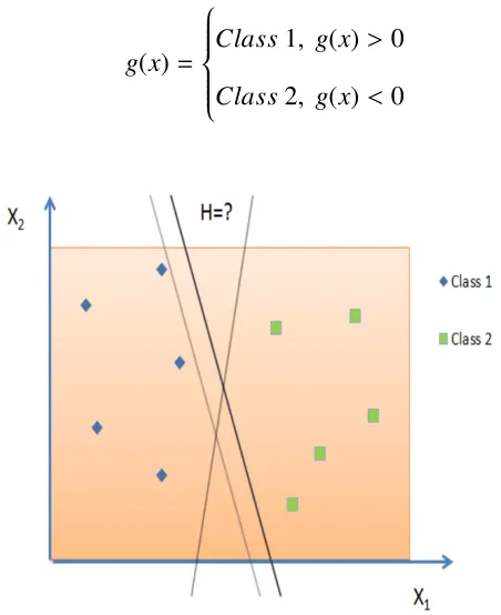
Support vector machines (SVMs) are a very useful tool in machine learning. Developed by Vapnik and Cortes [7] from statistical learning theory, it is a powerful method of supervised learning. Starting offwith discriminant analysis, assuming a set of data is linearly separable; that is, a hyperplane can be drawn that separates data given a set of inputsx = [x1,x2, ...,xn] a set of weightsw=[w1,w2, ...,wn] can be established to form a discriminant:

(37)

2.5. Bag ofWords 25

To find a decision rule:

g(x)=

            

Class1, g(x)>0

Class2, g(x)<0

(2.18)

Figure 2.10: A simple diagram of a Support Vector Machine with a separating plane in 2D

In Figure 2.10 the example is clearly linearly separable with the separating hyperplane said to be the discriminant. The problem arises in finding the ideal location of the discriminant function that will generalize well on new data by finding the ideal weights with respect to the given training data.

The idea is to write the discriminant as a linear combination of the data that lies closest to the separating hyperplane. These data points closest to the discriminant are known as support vectors. Given a training set of data for a binary classification problem:

yi =             

−1, Class1

+1, Class2

(2.19)

With the condition:

yi(wTx+w0)≥ b, b>0 (2.20)

(38)

Figure 2.11: The points lying closest to the separating hyperplane are deemed the support vectors

of the discriminant defines the marginm. The margin can be written asm= _|_W2_|. The problem can be reformulated as:

Minimize|w|sub ject to: yi(wTx+w0)≥b

(2.21)

In other words, minimizing the|w|translates to maximizing the margin separating the sup-port vectors. This can be modelled as a constrained quadratic optimization problem [20].

In many cases, the data may not be completely separable and a slack variable ξis used to provide a penalty for training examples that lie on incorrect sides of the discriminant. Using optimization techniques the SVM is computed by:

Minimize|w|sub ject to: 1

2w 2₊

CX i

ξi,

sub ject to:

yi(wTxi+b)≥ 1−ξi, whereξi ≥0∀i

(39)

2.5. Bag ofWords 27

The weight vector is given byW and biasb. This method can be solved analytically by the sequential minimal optimization technique developed by Platts [39] with complexityO(n3_).

2.5.5 Kernels

Most real world data is not linearly separable. In 1965 Thomas Cover proved that nonlinearly separable data is more likely to be linearly separable when cast into a higher dimensional space. This is known as Cover’s theorem [8]. By raising the dimensionality of the input space by the use of a kernel function allows the feature space to remain linear while increasing the likelihood of data separability. Selecting a kernel that corresponds to a dot product in a higher dimensional space is known as the kernel trick. A kernel function that is Positive Semidefinite (PSD) satisfies what is known as Mercer’s condition [3]. An example of raising the dimensionality of a binary class problem to a higher dimension making it linearly separable is given Figure 2.12 below by using the kernel functionK(x,x2):

Figure 2.12: Data that becomes linearly separable when mapped to a higher dimensional space

(40)

ide-ally one that satisfies Mercer’s condition. This allows for higher dimensional mappings of the data to take place with a simple modification to the comparison function that has an increased chance of being linearly separable.

2.6 First Order Information Encoding

Despite the success of the Bag of Words (BoW) representation it has remained relatively un-changed in retrieval and classification systems. One proposed method to help recover from the problem of quantization loss is to use first order information known by Vector of Locally Aggregated Descriptors(VLAD). This method proposed by Jegou et al. [25] is to extend the encoding of building a histogram of visual word occurrences found within an image. The pro-posed approach assigns each descriptor x ∈ Xto a centroid (using Nearest Neighbour) of a previously learned visual vocabulary as in Equation 2.15. After the assignment stage, the dif-ference between each descriptor and assigned centroid is computed forming a set of residual vectors. These two stages can be seen in Figure 2.13 and Figure 2.14.

(41)

2.6. FirstOrderInformationEncoding 29

Figure 2.14: VLAD stage 2: The residual vector of a single descriptor and its assigned centroid is a sub-vector which will then subsequently be aggregated.

The formal definition of the VLAD calculation:

vi,j =

X

NearestN(x)=ci

xj−ci,j (2.23)

With xj andci,j being the difference between each of the jthcomponents of the centroidci and the descriptor that is assigned to it. The resulting feature vector then has dimensionality D = k×d. Wheredis the length of the descriptor andkis the number of centroids.

(42)

2.7 Triangulation Embedding

So far, the BoW and VLAD encoding methods have been introduced. Triangulation embedding uses a different type of encoding method that operates on a per descriptor basis and is the core work of this thesis.

Two main approaches for determining the position of a point are: trilateration which finds points by a distance measure and the other is triangulation. Triangulation as recently described by Jegou and Zisserman [27] uses angles and will be our point of focus. In the proposed tri-angulation embedding strategy, a set of image descriptorsXare clustered using the traditional k-means approach. Once this is completed, a new set of image descriptors are then matched to the recently formed centroids. In the VLAD approach only the residuals of the query de-scriptors matched to the nearest centroid are computed. This approach deviates from VLAD because it does not use nearest neighbour assignment, but rather computes the residuals for each centroid.

There are two stages for this feature encoding method: embedding and aggregation. Their proposed embedding stepφ:Rd →RD(d< D) maps each descriptorx∈ Xas:

x7→φ(x) (2.24)

The aggregation stage is defined as a summation over all the mappings:

ψ(X)= X x∈X

φ(x) (2.25)

Given a set of visual words formed by k-means, C = {c1, ...,c|c|}i, ci R

D _{o f} _|_C_|_{. The} first step to defining the triangulation embedding functionφ4is computing a set of normalized

residual vectors from the descriptors as:

rj(x)=

(

x−cj

||x−cj||

)

, for j= 1...|C|, x_, cj (2.26)

(43)

2.7. TriangulationEmbedding 31

basis, whereas in the VLAD case, unit normalization is performed after the residual vectors are summed. This approach is also known assecant manifolds[21]. Other papers that use this technique outside of the computer vision area refer to these visual words learned by k-means as anchor points.

For each descriptor x ∈ X. It is important to point out that the unit ball is formed by quantizing residuals of image descriptors matched to the original dictionary on a validation set. For each subsequent descriptor to be embedded and later used for indexing or retrieval, the authors describe the triangulation embedding function, as:

φ4(x)= Σ−

1

2(R(_x)−R

0) (2.27)

With the R0 =EX[R(X)] andΣbelonging to the covariance matrix from a training set. This is typically referred to as whitening the vector. Where whitening is the process of centering, rotating and scaling the data defined as:

φ4(x)0 = diag(λ

−1₂

1 , ..., λ

−1₂

D ) P T _φ

(x) (2.28)

With λ being the largest eigenvalues and their associated eigenvectors from matrix P ∈

RD×D. The above equation shown by Jegou and Chum [23] can improve image retrieval and

research in [27] and [10] shows that the discriminative ability of the embedding is improved. It is also worth noting that selecting the firstneigenvectors such thatn < Djointly performs dimensionality reduction, later to be discussed in Section 2.9.

As the focus of this thesis is on image classification using multiple views, we proposed a method to aggregate the features from different views. For every view i in the image set, the features are whitened as described in Equation 2.28, using the same projection matrix P that is learned off-line across all views. The whitened feature vectors for each view are then concatenated to represent the image set:

Φ4(x) :=φ4i(x)0 f or i =1...n (2.29)

(44)

and 3.4% on the Oxford5k datasets. The authors provide a more rigorous explanation of the embedding step 2.24 and use a higher order representation leading to a weighted quadratic at the anchor points. In their publication they also prove that VLAD encoding is related to another very successful encoding method known asLocal Tangent-Based Coding(LTC) as introduced by Yu and Zhang [49]. LTC is based on the idea that features and codewords construct a smooth manifold. Through the use of anchor points, a nonlinear function f(x) on _Rd_{, that embeds} points onto the manifold can be approximated by a linear function onRD, whered < Dgiven

by Equation 2.28. The linear approximation of the nonlinear f(x) is given by f(x) ≈ PTφ₍_x_), wherePT is found by PCA.

All of these encoding strategies are derived from a common representation known asSuper Vector Encoding. The identifying characteristic of this set of encoding methods, is that all of these encoding methods use local information such as the residuals between the descriptor and nearest centroid (residual distance) to capture higher order information. The resulting feature vector has a dimensionality that is a factor of the dimensionality of the feature descriptor. Both the VLAD and Triangulation Embedding are examples of a Super-Vectors where both encoding methods capture local information between the descriptor and codeword. The original BoW representation that uses histogram encoding does not contain local information and is not con-sidered a Super-Vector because the feature vector depends on the number of centroids, not the dimensionality of the descriptor type.

(45)

2.8. PowerNormalization toAddressBurstyFeatures 33

2.8 Power Normalization to Address Bursty Features

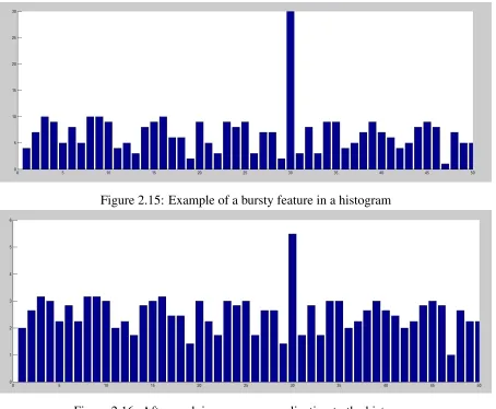
One of the phenomenons of feature detection is that once a feature is identified in an image there is a greater chance of a nearby feature (in the spatial sense) of also being detected with a high similarity score. This phenomenon is known asfeature burstsas analyzed by [24]. This can often result in large peaks in the feature vector which can corrupt the similarity metric that is in many kernel based learning approaches. The variance in the feature vector can be stabilized by applying power-law normalization defined as:

f(z)= sign(z)|z|α 0≤α≤1 (2.30)

Power normalization can be applied on each encoded descriptor individually or the feature vector. It is worth noting that when applied to the feature vector whenα=0.5 its known as the popular Hellinger Kernel.

Its worth noting that the peaks in the above images can occur from both the original BoW histogram component or they can occur from the vector residuals.

2.9 Dimensionality Reduction

One of the on going challenges in computer vision is that much of the data is inherently high dimensional and redundant. This raises the challenge of running time for many algorithms. Another problem is that as the dimensionality increases the distance between neighbouring data points grows exponentially. This is known as the curse of dimensionality. This problem is addressed by mapping the high dimensional data to a lower dimensional space based on the assumption that high-dimensional data lies near a lower-dimensional manifold.

One of the most common approaches to perform dimensionality reduction is to use Princi-pal Component Analysis (PCA). PCA attempts to find an orthogonal projection of the data onto a lower dimensional linear subspace fromn dimensions tod such thatn ≥ d while capturing the greatest variance in the data.

(46)

Figure 2.15: Example of a bursty feature in a histogram

Figure 2.16: After applying power normalization to the histogram

¯ x= 1

N N

X

n=1

xn (2.31)

With the mean-centered covariance defined as:

X

= 1

N−1 N

X

n=1

(xn− x¯)(xn− x¯)T (2.32)

For simplicity and keeping with common notation we will refer to the covariance matrix with mean subtraction along the columns asP

asXXT.

Singular Value Decomposition (SVD) is defined as taking a matrix X of size m x n and factoring it such that:

(47)

2.9. DimensionalityReduction 35

WhereU is amxmorthogonal matrix,V is anxnorthogonal matrix and S is a diagonal matrix whose diagonal elements are in decreasing order.

If the provided matrix to be decomposed is a square and symmetric matrix as in the case of XXT then SVD is equivalent diagonalization ofXXT byUresulting in each column vector ofu inUbeing eigenvectors. The numerical method to solving the SVD problem in this work was the use of the Jacobi Method.

The covariance matrixP

is symmetric of sizenxnand thus can always be diagonalized and diagonalized by an orthogonal matrix. Two matrices Aand Dare said to be similarAD˜ if an invertible matrix P exists such thatA= P−1DP

Figure 2.17: PCA example on a 2D dataset after projection of the data onto the principal component axes2

The principal components refer to the orthogonal vectors forming the new coordinate sys-tem spanned by the dominant eigenvectors of the data covariance matrix [15]. The eigenvectors capture the directions that maximize the variance in the data with a corresponding eigenvalue that captures the magnitude of variance. This example can be seen in Figure 2.17.

(48)

Part Classification on a Conveyor Belt

Framework

There has been previous research in using multiple view techniques for object recognition and retrieval tasks [14, 47, 40, 31, 30, 46]. It has already been demonstrated that the addition of multiple views within the BoW framework can improve accuracy for object classification as demonstrated by Savarese and Lei [45] and Fu et al. [14] on the same dataset. On other datasets, the task of object classification can be improved using multiple views as seen in the works of methods that rely on high quality reconstruction for classification, but 3D reconstruction is heavily affected by noise resulting in holes in the model in addition to being computationally more expensive. In many machine vision applications that require rapid classification using methods of 3D model generation are simply not practical when using standard cameras.

Many existing systems require the manufacturer of the vision system to create new tem-plates, or modify some parameters as most current systems use low level vision techniques. Our goal was to use computer vision techniques that could learn an additional object class dur-ing normal manufacturdur-ing production that could be performed with minimal supervision. This is often at the cost to the customer and possibly cause system downtime. Another real concern for manufacturers that do buy these vision systems is that computer hardware can break at any time without warning, in many cases halting production. The goal here was to create a setup that could address both of these problems.

(49)

3.1. PhysicalSetup 37

3.1 Physical Setup

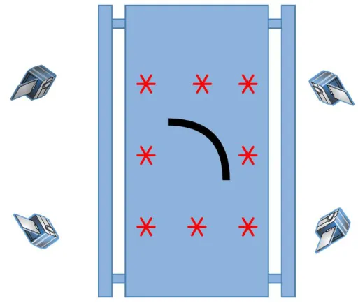
The purposed method of performing classification on a conveyor belt was to use multiple cam-eras to view the object from four sides. The motivation behind this was to make use of ad-ditional information that comes from multiple views and possible occlusions of discernible regions that may take place on the part. The occlusion of discriminating features on the object is very much a real case for the in-house dataset that was constructed. The hopes being that this approach would boost classification performance.

Figure 3.1: Positioned cameras focused over a conveyor belt

A diagram of the envisioned system can be seen in Figure 3.1 showing how the cameras were positioned around the conveyor belt to capture from the four corners. Naturally the four captured images provide a different view point of the object to be classified as can be seen in Figure3.2.

(50)

Figure 3.2: A diagram showing how different views can look drastically different depending on the view point

The cameras were positioned about 1.4 meters above the belt and angled at approximately 45◦ down towards the object. The spacing of the mounted cameras was arbitrarily selected to ensure the conveyor portion of the belt was always viewable. For consistency once positioned, the cameras were not moved.

The actual cameras themselves were simple, low cost, commercially available USB 2.0 web cameras. These cameras are able to record video in 1080p; however, all captured frames were processed and stored at a resolution of 1280x720. Many other works relating to multi view images require more specialized and costly cameras. The goal here being that the selection of cameras need not be expensive and provide a cost efficient solution. The type of camera used can be seen in Figure3.4.

3.2 Object Localization

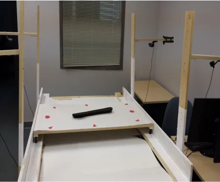
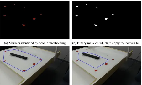
Given that the cameras are positioned above the conveyor belt at an angle, there are regions outside of the belt that are captured. Since the regions offof the belt provide no additional information about the part red patches as seen in Figure 3.3 were placed on the belt surrounding the object. As the focus of this work is on the classification aspect of the problem and not image segmentation the red markers served to provide a simple boundary of the object.

(51)

3.2. ObjectLocalization 39

Figure 3.3: Mock conveyor used in lab to gather data.

creates the binary mask. Given three discrete sets Θ = {θ1, θ2, θ3} representing each colour channel, segmentation by colour thresholding is defined as:

g(x,y)=

            

1 : f(x,y) ⊆ Θ

0 : f(x,y) * Θ

(3.1)

To reduce the number of spurious pixels being identified as the markers the basic noise reduction technique of median filtering was applied as a preprocessing step. One of the masks generated can be seen in Figure 3.5b.

(52)

Figure 3.4: The type of camera used in our experiments1

as seen in 3.6a. Given a set of n points corresponding to pixels for which g(x,y) = 1 the computational complexity of finding the hull isO(nlogn) based on the Graham method [17].

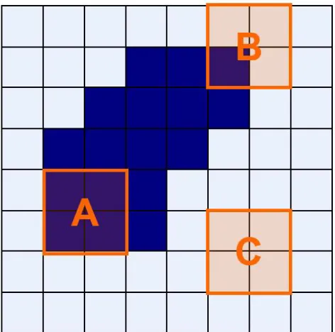
At this stage the current mask contains the image but also may contain some markers that fall within the hull. We remedied this problem by applying the morphological operation of erosion. Since the hull could take on various shapes depending on the image captured we needed to shrink the size of the mask while preserving its shape. The convex hull could vary widely among views as it relates to the position of the belt and shrinking the mask by a set amount of pixels runs the risk of masking out some of the auto part in the image. This approach helps to minimize the impact of this problem. At this point only features within the masked region will be detected shown in Figure 3.5d.

Using the definition from Woods and Gonzalez [16], erosion stems from set theory and is defined given two setsAandBinZ2the erosion ofAbyBdenotedA Bis given by:

A B={z|(B)z ⊆ A} (3.2)

SetBis commonly called a structuring element. In the context of digital imagesBis amxn

(53)

3.2. ObjectLocalization 41

(a) Markers identified by colour thresholding (b) Binary mask on which to apply the convex hull

(c) Object enclosed by the hull shown in blue (d) Reduced area to only enclose the part

Figure 3.5: The object localization process

matrix and is the set of all points, that when translated byzis contained inA.

Using the definition of a digital image from Section 2.2.1 given imageAand treating it as a function corresponding to (x,y) pixels the result of performing erosion overAwith structuring elementBreturns a maskggiven by:

g(x,y)=

            

1 : if B fits A

0 : ifBdoes not fit A

(3.3)

(54)

(a) Convex hull (b) Distance map of the hull after erosion

Figure 3.6: The shrinking of the hull by erosion

3.3 Extension to Multiple Views

Historically, most problems in computer vision involving the use of stereo or multi view images try to compensate from the fact that we live in a 3D world and when taking images 3D points are mapped to a 2D plane, for the standard camera model resulting in a loss of depth information.

The basics of how a camera works come from the pinhole camera. The same concept takes place when working with digital images. Multiple Rays of light emanates from a single point known as the point source. The concept of a pinhole camera is to capture only a single ray from each point on the object. The model lets rays of light into a small opening in a light proof box that inverts the image. The opening of the box that allows light in is called the aperture. An ideal pinhole camera has an infinitely small aperture that will only allow one ray to pass through. Realistic cameras based on this model are not ideal and have more than one ray per point entering the aperture. Small apertures allow less rays in resulting in a darker but more focused image. Larger apertures allow for a brighter but more blurry image.

The pinhole camera model does allow for an approximation of a perspective projection for generating an image. The mapping of the object to the image plane can be see in Figure 3.9. Its worth noting that in this diagram the image plane is actually in front of the camera.

(55)

3.3. Extension toMultipleViews 43

Figure 3.7: Structuring elements note that element A fits whereas B and C do not.2

                 f x f y z                  =                 

f 0 0 0 0 f 0 0 0 0 1 0

                                          x y z 1                          (3.4)

The above formulation can be rewritten as:

zm=PM (3.5)

Most cameras do not use an actual pinhole to filter rays of light but make use of a lens for the purpose of focusing the rays of light as seen in Figure 3.10

The matrix mcan simply be rewritten asm = (f x/z, f y/z,1)T_{. The drawbacks regarding} this formulation is it lacks camera pose and internal geometry. Through matrix decomposi-tion of matrix Pthe decomposition can give intrinsic and extrinsic parameters. The intrinsic matrix contains internal parameters such as focal length. The extrinsic matrix contains param-eters used to define motion about a static scene relating the world coordinates to the camera

(56)

Figure 3.8: Pinhole

Figure 3.9: Projection diagram

coordinates.

These camera parameters can be found through a process known as camera calibration. The distortion coefficients can be identified by both sets of parameters and corrected for. Glossing over the details of camera calibration it is important to point out that this plays a very important role in recovering depth. Most of the techniques above would require the use of calibration for whatever multi view information they deal with.

(57)

3.3. Extension toMultipleViews 45

Figure 3.10: Lens used to focus light3

between some of the part classes could only be identified when looking at the object from multiple view points.

This is where this work deviates from many of the above approaches. Many techniques for generating 3D models require many views of the part. This is evident by the large number of views of the same object in publicly available datasets. Many stereo imaging techniques have two cameras very close together. The objects in-house dataset can only be distinguished at a visual level when the views are angled far apart as in our setup. Other feature based techniques to work on the correspondence problem between sets of features across multiple views relies on strong discriminative features. Unfortunately our objects for classification are all black and have some level of luster. Reliable feature matching techniques are not feasible as with most reconstruction methods using correspondence when there are not enough features matched consistently across the frames with high confidences they are dropped. The end result is an extremely sparse point cloud representation with very few points and certainly not enough points to regenerate the full model. There is of course the technique of deflectometry [29] uses very specialized equipment for paint defects after performing surface reconstruction. The main issue with that approach is the object needs to be stationary. Even if the common 3D approach for image classification could be reliably performed our system requires classification of the

(58)

Feature Encoding Strategies for Multi-View Image Classification

Scholarship@Western

Scholarship@Western

Feature Encoding Strategies for Multi-View Image Classification

Feature Encoding Strategies for Multi-View Image Classification

Acknowledgements

Contents

List of Tables

Chapter 1

Introduction

1.1

Motivation

1.1.1

Problem Statement

1.2

SIFT, SURF, and ORB features

1.2.1

SIFT features

1.2.2

SURF features

1.2.3

ORB features

1.3

Thesis Contribution

1.4

Organization of thesis

1.5

Experiment Summary

Chapter 2

Background and Literature Review

2.1

Machine Learning

2.2

Image Processing, Understanding and Computer Vision

2.2.1

Image Representation

2.3

Feature Extraction

2.4

ORB Features

X

X

X

X

2.5

Bag of Words

2.5.1

Descriptor Quantization

2.5.2

Histogram Encodings

2.5.3

Spatial Pyramids and Pooling

2.5.4

Support Vector Machines

2.5.5

Kernels

2.6

First Order Information Encoding

2.7

Triangulation Embedding

2.8

Power Normalization to Address Bursty Features

2.9

Dimensionality Reduction

Part Classification on a Conveyor Belt

Framework

3.1

Physical Setup

3.2

Object Localization

3.3

Extension to Multiple Views