Fundamental Classifications for Empirical Study Data Mining

(1)

Available online: https://edupediapublications.org/journals/index.php/IJR/ P a g e | 314

Fundamental Classifications for Empirical Study Data Mining

Prof.Dr.G.Manoj Someswar

1

, Dr.Mukiri Ratna Raju

2

1. Dean (Research), Global Research Academy – Scientific & Industrial Research

Organisation[Autonomous], Hyderabad, Telangana State, India

2. Associate Professor, Department of CSE, St.Ann’s College of Engineering &

Technology, Chirala, Andhra Pradesh, India

Abstract

Dimensionality diminishment through the determination of an applicable quality (component) subset may deliver different advantages to the real information mining step, for example, execution change, by easing the scourge of dimensionality and enhancing speculation abilities, accelerate by lessening the computational exertion, enhancing model interpretability and decreasing expenses by maintaining a strategic distance from "costly" elements. These objectives are not completely perfect with each other. Consequently, there exist a few component determination issues, as indicated by the particular objectives. In our research paper, include determination issues are characterized into two fundamental classifications: finding the ideal prescient components (for building productive expectation models) and discovering all the applicable elements for the class quality.

From a simply hypothetical point of view, the determination of a specific trait subset is not of enthusiasm, since the Bayes ideal forecast control is monotonic, consequently including more components can't diminish precision. Practically speaking, be that as it may, this is really the objective of highlight choice: choosing the most ideal property subset, given the information and learning calculation qualities, (for example, inclinations, heuristics). Regardless of the possibility that there exist certain associations between the characteristics in the subset returned by a few strategies and the hypothetically significant properties, they can't be summed up to shape a useful technique, material to any learning calculation and dataset. This is on account of the data expected to register the level of importance of a characteristic (i.e. the genuine dissemination) is not by and large accessible in commonsense settings.

Keywords: Feature Selection Techniques,CFS (Correlation-based Feature Selection), Wrapper

(2)

Introduction

The idea of pertinence is fundamental to the hypothetical detailing of highlight determination. There are a few meanings of importance accessible in writing. In [Gen89], an element is characterized as significant if its esteems shift deliberately with the class characteristic esteems. In this is formalized as:

Definition 1:

Xj

is

relevant iff



x and y for which p(Xj = x )>0, s.t. p(Y = y | Xj = x ) ≠ p(Y = y),

meaning that an attribute is relevant if the class attribute is conditionally dependent on it. Another possible definition of relevance is that by removing attribute Xj from the

feature set F the conditional class probability changes :

Definition 2:

Xi

is

relevant iff

 x, y and f for which p(Xj = x, Fj= f )>0, s.t. p(Y = y | Xj = x, Fj= f ) ≠ p(Y = y | Fj = f) where

Fj = {X1, ... Xj-1, Xj+1,, ... Xn} denotes the set of all attributes except Xj and f represents a value

assignment to Fj.

However, these definitions may yield unexpected results. Take the Boolean xor problem, for example, with Y = X1X2. Both X1 and X2 are indispensable for a correct prediction of Y. However, by the first definition, both X1

and X2 are irrelevant, since p(Y=y | X1= x) = p(Y=y)= 0.5, i.e. for any value X1there are two different values

for y. The same is true for X2. Also,if we add feature X3=X2, then by the second definition, both X2 and X3 are

considered irrelevant, since neither adds information to F3 and F2, respectively.

To address such issues, in two degrees of relevance are introduced: strongrelevance and weak relevance, by quantifying the effect of removing the attribute on theperformance of the Bayes optimal classifier.[1] Thus, an attribute is strongly relevant if it indispensable, i.e. its removal results in performance loss of the optimal Bayes classifier. The actual definition is equivalent to the second definition of relevance presented before.

The definition for weak relevance is the following:

Definition 3: An attribute Xj is weakly relevant iff it is not strongly relevant and  a

subset of features Fj’ of Fj for which  x, y and f’ with p(Xj = x, Fj’ = f ‘)>0, s.t. p(Y = y | Xj =

x, Fj’ = f ‘) ≠ p(Y = y | Fj’ = f ‘)

(3)

is strongly relevant, and X2 and X3 are weakly relevant.

The above definitions of relevance do not imply attribute usefulness for a specific learner. Therefore, we define feature selection in the following manner:

Definition 4: Feature selection represents the extraction of the optimal attribute subset,

Fopt = {Xk1, ..., Xkn}, where {k1, ..., kn}  {1,...,n}

The definition of optimality is specific to the feature selection technique (on the subset evaluation measure), and it depends on the learning algorithm characteristics (such asbiases, heuristics) and on the end goal of the classification.[2]

Feature Selection Techniques

There exist two possible methodology to take after for highlight assurance: examine for the best subset of judicious segments (for building successful desire models), or find all the pertinent components for the class quality. The latter is proficient by playing out a situating of the credits as shown by their individual perceptive power, surveyed by methods for different procedures: (i) figure the execution of a classifier worked with each single variable, (ii) enlist estimation measures, for instance, an association coefficient or the edge and (iii) use information speculation measures, for instance, the basic information. Include choice calculations are customarily separated in machine learning writing into: channel techniques (or channels), wrapper strategies (or wrappers), and implanted techniques (i.e. techniques installed

inside the learning procedure of specific

classifiers).

In any case, this approach fails to perceive abundance parts, which have been seemed to hurt the portrayal technique of the naïve Bayes classifier. Thusly, most part decision strategies focus on checking for the best subset of insightful components. They change in two fundamental perspectives: the interest methodology used and the trademark subset evaluation system.

There exist a couple of broad audits on highlight assurance counts in composing. Dash masterminds highlight assurance counts using two criteria: the period strategy and the evaluation work. Three time procedures – heuristic, complete and self-assertive – and five appraisal measures – evacuate, information, dependence, consistency and classifier botch rate – are perceived. This results in fifteen

(4)

class are overviewed.[3] Trial appraisals are performed on three fake datasets, to think the farthest point of each estimation to pick the pertinent parts. Another careful review is presented in the portrayal of highlight assurance figurings presented there resembles that the refinement is that the period philosophy is furthermore divided into chase affiliation and time of successors, realizing a 3-estimation depiction of the component assurance procedures. Other beneficial audits can be found in our research paper.

For the element determination issue, the request of the hunt space is O(2|F|). Along these lines, playing out a comprehensive scan is unfeasible aside from spaces with few components. Finish look systems play out a total scan for the ideal subset, as per the assessment work utilized. Their multifaceted nature is littler than O(2|F|), on the grounds that not all subsets are assessed. The optimality of the

arrangement is ensured. Delegates of this class are: branch and bound with backtracking or

expansiveness initially look.

A more proficient exchange off between arrangement quality and inquiry unpredictability is given by heuristic hunt strategies. With a couple of exemptions, all pursuit techniques falling in this classification take after a basic procedure: in every cycle, the rest of the components to be chosen/rejected are considered for choice/dismissal. The request of the look space for these strategies is

for the most part quadratic in the quantity of

elements – O(|F|2). In this manner, such

strategies are quick, and despite the fact that

they don't ensure optimality, the nature of the arrangement is normally great. Illustrative of this classification are: insatiable slope climbing, which considers nearby alterations to the element subset (forward choice, in reverse end or stepwise bi-directional pursuit), best-first inquiry, which additionally rolls out neighborhood improvements yet permits backtracking along the hunt way and hereditary calculations, which consider worldwide changes. Sufficiently given time, best-first hunt will play out a total pursuit. Covetous slope climbing experiences the skyline impact, i.e. it can get gotten at nearby optima. Sufficiently given hunt fluctuation, populace size and number of cycles, hereditary calculations as a rule join to the ideal arrangement.

(5)

ravenous slope climbing can be infused with irregularity by beginning from an underlying

arbitrary subset.

Whether or not a certain sub-set is optimal depends on the evaluation criterion employed. The relevance of a feature is relative to the evaluation measure.

Since, most often, the end goal of feature selection is to obtain an efficient classification model in the processing phase, setting the target of feature selection to minimize the (Bayesian) probability of error might be appropriate. The probability of error is defined as :

Pe =



[1



max

P

(

y

k

|

x

)]

p

(

x

)

dx

K c

unconditional probability distribution of the

instances, and P(yk_{| x)}_{is the posterior probability where}

p(x) = k 1p(x | yk )P( yk ) is the of yk being the class of x.

The goodness of a feature subset F’ is therefore: J = 1 – Pe. P(yk| x) are usually unknown, and have to

be modeled, either explicitly (via parametric or non-parametric methods), or implicitly, by building a classification model which learns the decision boundaries between the classes on a sample dataset. For a feature subset F’, an estimate Pe of

the error is computed, by counting the errors produced by the classifier built on a subset of the available data, using only the features in F’, on a holdout test set taken also from the available data. The feature subset which minimizes the error

returned. This forms the basis of the wrapper methodology. The estimation of Pe may require

more sophisticated procedures than simple holdout validation set: k-fold cross-validation or repeated bootstrapping may yield more accurate values.

Distance (or discrimination, separability) measures favor features which induce a larger distance between instances belonging to different classes. The Euclidean distance is one of the metrics used to compute the distance. The best feature subset is that which maximizes the inter-class distance:

(6)

J





k1

P

(

y

k

)



lk1

P

(

y

l

)

D

(

y

k

,

y

l

)

where

y

k

and

y

l

represent the

k

th

and

l

th

class labels, respectively, and

D

(

y

k

,

y

l

)



1

_N _N



k k



kl k1 d(x(k ,k1 )

,x (l ,k2 )

)

N

k

N

l 1 2 1

represents the interclass distance between the kth

and lth_{class labels,}_N

k and Nl are the numberof

instances belonging to classes Nk and Nl,

respectively, and x(k,k1) is the instance k1 of class yk.

Such measures do not necessitate the modeling of the probability density function. As a result, their

relation to the probability of error can be loose Divergence measures are similar to distance measures, but they compute a probabilistic distance between the class-conditional probability densities:

J





f

[

p

(

x

|

y

k

),

p

(

x

|

y

l

)]

dx

Classical choices for f include: the Kullback-Liebler divergence or the Kolmogorov distance. Such measures provide an upper bound to Pe. Statistical dependence quantify how strongly two features are associated with one

another, i.e. by knowing the value of either one, the other can be predicted. The most employed such measure is the correlation coefficient:

Correlation(Xi, Xj)

=

E[( X i 



X )( Xj 



Xj )] i



Xj

X

i

(7)

Available online: https://edupediapublications.org/journals/index.php/IJR/ P a g e | 320 m

(

x

k(i)



x

(i)

)(

x

k(j)



x

( j

)

r

x(i)x(j)





k 1

(

m



1)

s

x(i)

s

x(j)

where x(i)_and_x(j)_{represent the value sets of attributes}_X

i and Xj, respectively, x(i) and

x( j

) represent the sample means and sx(i) and sx( j ) represent the sample standard deviations.

This measure may be used in several ways: rank features according to their individual correlation with the class – those exhibiting a large correlation are better; a second possibility is investigated in, where the heuristic “merit” of a subset of features is proposed, according to which subsets whose features exhibit higher individual correlation with the class and lower inter-correlation receive higher scores:

M

F'



k r

cf

k



k

(

k



1)

r

ff

where k = |F’|, r represents the sample correlation coefficient, c represents the class and f represents a predictive feature; rcf is the mean feature-class correlation, fF ' and rff is the mean feature-feature inter-correlation.

Similar to the statistical dependence measures, there are several measures from information theory, based on Shannon’s entropy, which can help determine how much information on the class Y has been gained by knowing the values of Xi. The most employed is the information gain, which can be used without knowledge

of the probability densities, such as in decision tree induction.

Consistency measures are characteristically different than all the other evaluation measures. They rely heavily on the training data. Also, the methods that employ them apply the Min-Features bias, i.e. favor consistent hypotheses definable over as few features as possible. An inconsistency in F’ appears when two instances belonging to different classes are indistinguishable by their values of the features in F’ alone. The inconsistency count of an

instance xi with respect to feature subset F’ is:

(8)

k

where F’(xi) is the number of instances in training set T equal to xi using only attributes in F’,

and F '

k

(x ) is the number of instances in T of class yk_{equal to}_xi_{using only the features in}

i

F’. The inconsistency rate of a subset of features F’ in the training set T is expressed as the average of the inconsistency scores of T’s instances with respect to F’. This is a monotonic measure, which has to be minimized.

Filter Methods

Channels perform include determination freely of a specific classifier, being spurred by the properties of the information dispersion itself. There are a few powerful calculations in writing which utilize a channel technique. Among the most referred to are: RELIEF , LVF, FOCUS Correlation-based channel – CFS or measurable strategies in light of theory tests. [4]

Help depends on the thought utilized by closest neighbor learners: for each case in a haphazardly picked test, it registers its closest hit (nearest case from a similar class) and miss (nearest case from an alternate class), and uses a weight refresh instrument on the components. After all the preparation occasions in the specimen have been dissected, the components are positioned by their weights.[5] The impediments of this technique originated from the way that inadequate examples may trick it, and there is no broad philosophy for picking the specimen measure.

LVF (Las Vegas Filter) utilizes a probabilistically-guided irregular inquiry to investigate the characteristic subspace, and a consistency

assessment measure, unique in relation to the one and utilized by FOCUS. The strategy is productive, and has the upside of having the capacity to discover great subsets notwithstanding for datasets with clamor. Additionally, a great estimation of the last arrangement is accessible amid the execution of the calculation.[6] One downside is the way that it might take more time to discover the arrangement than calculations utilizing heuristic era methods, since it doesn't exploit earlier learning.

(9)

the gathering trait class connection against property characteristic relationship is figured, as in condition [7] The subset which expands the proportion is the decreased trait set. PCA (Principal Components Analysis) is a channel strategy generally utilized for highlight determination and extraction in picture handling applications (numeric qualities). It plays out an orthogonal change on the info space, to deliver a lower dimensional space in which the principle varieties are kept up. There are a few unique renditions to perform PCA – a survey on a few methodologies is accessible in our research paper.

Wrapper Methods

Since channels neglect to catch the inclinations innate in learning calculations, with the end goal of boosting the grouping execution, channel strategies may not accomplish critical enhancements. Rather, wrapper techniques ought to be considered. Test comes about which approve this suspicion can be found in our research paper. Wrappers instead of channel strategies, look for the ideal subset by utilizing an experimental hazard assess for a specific classifier (they perform observational hazard minimization).[8] Consequently, they are

changed in accordance with the particular relations between the arrangement calculation and the accessible preparing information. One disadvantage is that they have a tendency to be fairly moderate.

By and large wrapper technique comprises of three

fundamental strides: • area system

• an assessment system • an approval system

Along these lines, a wrapper is a 3-tuple of the shape <generation, assessment, validation>. The component choice process chooses the insignificant subset of elements, considering the expectation execution as assessment capacity: limit the evaluated blunder, or proportionately, amplify the normal precision.

Each chose highlight is thought to be (emphatically) pertinent, and rejected elements are either unimportant or repetitive (with no further refinement). The distinctions in the utilization of the wrapper approach are because of the strategies utilized for era, the classifier utilized for assessment and the system for evaluating the off-example exactness.

The era strategy is an inquiry method that chooses a subset of elements (Fi) from the first list of

capabilities of the set (

F

),

Fi



F

, as exhibited in

(10)

On account of wrappers the assessment is performed by measuring the execution of a specific classifier on the projection of the underlying dataset

on the chose traits (i.e. evaluate the likelihood of blunder, as exhibited in area 4.2.2)[9]. The approval system tests the legitimacy of chose subset through examinations gotten from other component determination and era methodology sets. The goal of the approval technique is to recognize the best execution that could be acquired in the initial two stages of the strategy for a given dataset, i.e. to recognize the determination strategy which is most reasonable for the given dataset and arrangement technique. As an outcome, the insignificant component subset is chosen. All components from the subset are viewed as pertinent to the objective idea. Besides, the grouping technique plays out the best, so it is to be considered for further arrangements.

The underlying work on wrappers has been done by John, Kohavi and Pfleger , which directed a progression of investigations to concentrate the impact of highlight determination on the speculation execution of ID3 and C4.5, utilizing a few counterfeit and characteristic space datasets. [10] The outcomes demonstrated that, with one special case, highlight determination did not change the speculation execution of the two calculations fundamentally. Hereditary pursuit techniques were

utilized in inside a wrapper system for choice tree learners (SET-Gen), trying to enhance both the exactness and effortlessness of the subsequent models. The wellness work proposed by the creators was a direct blend of the exactness, the span of the subsequent trees (standardized by the preparation set size) and the quantity of components.

Insensibility has been proposed in to ease the impact of unessential elements on the kNN classifier. The calculation utilizes in reverse end as era strategy and an unmindful choice tree as classifier. A setting touchy wrapper for example based learners is proposed in, which chooses a (conceivably) unique subset of elements for each occasion in the preparation set. In reverse disposal

(11)

a hazard gauge (i.e. wrapper based), however the strategy can be utilized likewise to create a positioning of the components. [11]

The most essential feedback conveyed to the wrapper approach is worried with its computational cost, since each component subset must be assessed via preparing and assessing a classifier, conceivably a few times (if cross-approval, or rehashed bootstrapping are utilized). To address this issue, effective pursuit techniques have been proposed in our research paper – race seek and schemata look – and – compound hunt space administrators. Also, eager inquiry procedures have a lessened time many-sided quality and appear to be powerful against over fitting.

Combining Generation Strategies

A first inspiration for handling a blend approach for the era systems can be found in the without no lunch hypothesis. It is realized that, because of the particular predominance of classifiers, there is no

generally best technique, i.e. one which yields better execution than every other strategy, on any issue. Instinctively, this issue ought to influence the era techniques utilized as a part of highlight choice too. As will be appeared in segment 4.3.2, there is no prevalent wrapper mix, in spite of the fact that there are sure mixes which continually yield great

execution change. Diverse pursuit systems in the era step may yield essentially unique outcomes.

A moment inspiration for such an approach is the way that mix techniques by means of outfit learning or the Dempster-Shafer Theory of Evidence have been appeared to enhance the strength of individual classifiers over an extensive variety of issues. Such methodologies decrease the fluctuation related to single learners, and by consolidating distinctive techniques the subsequent inclination is relied upon to be lower than the normal predisposition of the individual strategies.

(12)

(13)

COMBINE GENERATION STRATEGIES

Given: Set

Sp



{

Sp

1

,

Sp

2

,...,

Sp

p

}

of search strategies sEval – subset evaluation method

T – training set Do:

1. Generate individual feature subsets corresponding to each search method, using sEval and T:



{

F

CV1

,...,

F

CVp

}

, where

F

k F

CV



{(

X

j

,

cv

)

k

_|

_j

_

_1,

_n

_}

CV j

cv

jk- local score of attribute Xjin set

F

CVk

2. Compute, for each attribute, a global score: p

s

j







k

cv

kj

k1

3. Select the final attribute subset:

F



{

X

j

|

s

j





j

}

where



j is the selection threshold for attribute Xj

One way to deal with create such a component subset is to run the wrapper in a cross-approval circle and relegate to each element a score equivalent to the quantity of folds in which it was chosen. Utilizing the neighborhood choice scores, we figure a worldwide weighted score for each element, and apply a determination procedure to acquire the last element subset. As of now, a better than expected uniform choice methodology has been connected, however the strategy can be stretched out to suit other voting methodologies. Experimental Evaluation

Evaluating the Wrapper Methodology

A progression of assessments on the wrapper technique have been led keeping in mind the end

(14)

highlight determination around choice trees. The issue was initially figured in, where it was demonstrated that pruning ought to be maintained a strategic distance from for this situation.

(15)

In the endeavor to give answers to these inquiries, a progression of relative assessments on a few instantiations of the wrapper strategy have been performed. Fourteen UCI datasets were utilized, portrayed in Table A. 4.1. In choosing the datasets, the criteria expressed in were utilized: dataset measure, sensible encoding, fathomability, non-detail and age. The assessment situations have been set up utilizing the WEKA system. Taking after a progression of preparatory assessments on a few pursuit methodologies, covetous stepwise in reverse hunt and best initially look have been chosen as era strategies. Three distinctive learning plans, speaking to three conspicuous classes of calculations: choice trees (C4.5 – amendment 8 – J4.8, as actualized by WEKA); Naïve Bayes and troupe techniques (AdaBoost.M1, with Decision Stump as a base learner) were utilized for the assessment and approval strategies. For J4.8, investigations were performed both with and without pruning.[14]

In introducing the outcomes, the accompanying

truncations have been utilized:

 for the era technique: o BFS: best initially seek

 GBW: avaricious stepwise in reverse inquiry

 for the assessment work and the approval technique: o JP: J4.8 with pruning

 oJNP: J4.8 without pruning o NB: Naïve Bayes

 AB: AdaBoost.M1

A "_" is utilized to flag a "couldn't care less" circumstance (e.g. all mixes yield similar outcomes).

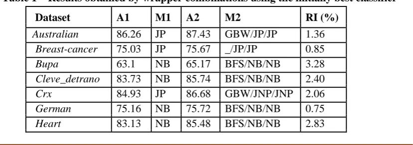
Table 1 presents the outcomes acquired by wrappers utilizing the classifier which at first yielded the most astounding precision for the assessment and approval methods. In everything except two cases we find that the exactness increments in the wake of performing highlight determination utilizing the wrapper approach on the at first best classifier.

Table 1 – Results obtained by wrapper combinations using the initially best classifier

Dataset A1 M1 A2 M2 RI (%)

Australian 86.26 JP 87.43 GBW/JP/JP 1.36

Breast-cancer 75.03 JP 75.67 _/JP/JP 0.85

Bupa 63.1 NB 65.17 BFS/NB/NB 3.28

Cleve_detrano 83.73 NB 85.74 BFS/NB/NB 2.40

Crx 84.93 JP 86.68 GBW/JNP/JNP 2.06

German 75.16 NB 75.72 BFS/NB/NB 0.75

(16)

Cleveland 56.54 NB 60.71 GBW/NB/NB 7.38

Monk3 98.91 JP 98.92 _/J_/J_ 0.01

PimaDiabethes 75.75 NB 77.58 BFS/NB/NB 2.42

Thyroid 99.45 AB 99.28 BFS/J_/J_ -0.17

Tic-tac-toe 83.43 JP 83.47 BFS/J_/JNP 0.05

Vote 96.22 JP 96.73 GBW/JP/JP 0.53

Wisconsin 96.24 NB 96.07 BFS/NB/NB -0.18

A1 = Initial best accuracy; M1 = Initial best classifier; A2 = Accuracy for the wrapper method which uses the initial best classifier for both evaluation and validation; M2 = Wrapper method which uses the initial best classifier for both evaluation and validation; RI = Relative Improvement (%) = (A2-A1)/A1

Table 2 – Datasets used in the evaluations on wrapper feature selection

Dataset No. No. Attributes

Attributes Instances type

Australian 14+1 690 Num, Nom

Breast-cancer 9+1 286 Nom

Bupa 5+1 345 Num

Cleve-detrano 14+1 303 Num, Nom

Crx 15+1 690 Num, Nom

German 20+1 1000 Num, Nom

Heart 13+1 270 Num, Nom

Cleveland 13+1 303 Num, Nom

Monk3 7+1 432 Nom

Pima Diabethes 8+1 768 Num

Thyroid 20+1 7200 Num, Nom

Tic-tac-toe 9+1 958 Nom

Vote 16+1 435 Nom

Wisconsin 9+1 699 Num

On the Thyroid dataset no change is found. This conduct is clarified by the high starting precision. Because of that esteem, enhancements are hard to get. Along these lines, there is no explanation

(17)

different mixes utilized for the wrapper prompt an exactness increment on this dataset too (see table 2). Table 2 presents the outcomes gotten by the best <generation, assessment, validation> mixes. In the majority of the cases, the BFS/NB/NB mix accomplishes the most elevated precision, while mixes utilizing JP or JNP come in second. There are three special cases to this run the show:

• the Breast-tumor dataset: the main dataset on which mixes utilizing AB acquire the most elevated exactness

• the Cleveland dataset: here, GBW acquires the best precision. Likewise, the Cleveland dataset is the just a single in which GBW chose less qualities than BFS.

• the Wisconsin dataset: as indicated prior, for this set a blend of classifiers in the assessment/approval steps accomplishes the most

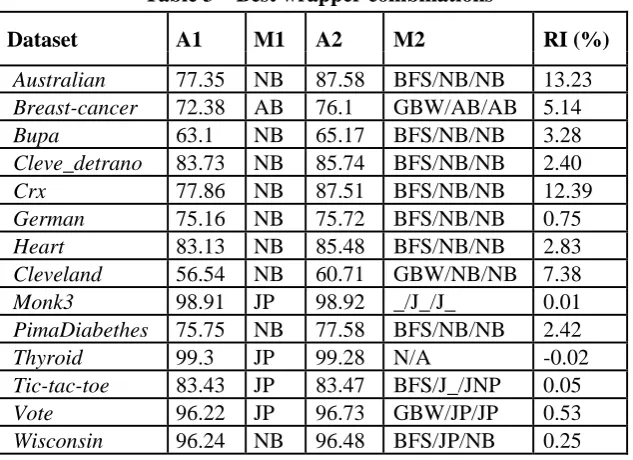
elevated exactness. Table 3 presents the outcomes acquired by the _/JNP/JNP wrapper. The considerable preferred standpoint of this wrapper is that it is to a great degree stable. It always helps the precision, despite the fact that it doesn't acquire the best change constantly. The _/J_/J_ wrappers get the best exactnesses on 4 datasets (out of 14), while in 1 case the best precision is acquired with a wrapper utilizing J4.8 as assessment capacity. Besides, on 8 datasets, a wrapper in view of J4.8 gets the second best execution, while on 2 different datasets, it is considered as assessment capacity, or approval work separately. The best relative

(18)

(19)

Table 3 – Best wrapper combinations

Dataset A1 M1 A2 M2 RI (%)

Australian 77.35 NB 87.58 BFS/NB/NB 13.23

Breast-cancer 72.38 AB 76.1 GBW/AB/AB 5.14

Bupa 63.1 NB 65.17 BFS/NB/NB 3.28

Cleve_detrano 83.73 NB 85.74 BFS/NB/NB 2.40

Crx 77.86 NB 87.51 BFS/NB/NB 12.39

German 75.16 NB 75.72 BFS/NB/NB 0.75

Heart 83.13 NB 85.48 BFS/NB/NB 2.83

Cleveland 56.54 NB 60.71 GBW/NB/NB 7.38

Monk3 98.91 JP 98.92 _/J_/J_ 0.01

PimaDiabethes 75.75 NB 77.58 BFS/NB/NB 2.42

Thyroid 99.3 JP 99.28 N/A -0.02

Tic-tac-toe 83.43 JP 83.47 BFS/J_/JNP 0.05

Vote 96.22 JP 96.73 GBW/JP/JP 0.53

Wisconsin 96.24 NB 96.48 BFS/JP/NB 0.25

A1 = Initial accuracy for the classifier used in the best wrapper; M1 = Classifier of the best wrapper; A2 = Accuracy for best wrapper; M2 = Best wrapper; RI = Relative Improvement

Table 4 – Results obtained by the _/JNP/JNP wrapper

Dataset Initial BFS GBW Dataset Initial BFS GBW

Australian 86.2 86.26 86.03 Cleveland 53.46 53.32 59.55

Breast-cancer 73.68 75.03 75.19 Monk3 98.91 98.92 98.92

Bupa 59.13 64.80 64.80 PimaDiabethes 73.82 73.35 74.00

Cleve_detrano 76.63 82.08 80.33 Thyroid 99.3 97.73 97.78

Crx 84.93 86.14 86.68 Tic-tac-toe 83.43 83.47 83.47

German 71.72 73.11 72.26 Vote 96.22 96.64 96.66

(20)

Table 4 demonstrates how the quantity of characteristics is fundamentally lessened through component choice (54.65% and 52.33% overall, for the best wrapper, and individually second best wrapper). This restricts the pursuit space and accelerates the preparation procedure. For the most part, BFS chooses less traits than GBW, and the subsequent datasets end up being more proficient. The special case is the Cleveland dataset, for which GBW chooses less properties than BFS. For this situation additionally the execution is better. The general conclusion is that less credits prompt a superior execution (both expanded exactness and diminished preparing time). [15]

Table 5 demonstrates the first and second best exactnesses acquired after element choice. It can be watched that the second best change is huge also, which shows that element determination ought to be utilized as a part of any information mining process, paying little heed to how great the accessible learning calculation is.

Evaluating the Combination Strategy

A progression of assessments on 10 UCI benchmark datasets have been performed, to

investigate the impacts delivered by the proposed blend technique on the order execution of J4.8. Four distinctive inquiry systems have been viewed as: best-first hunt (bfs), bi-directional best-first pursuit (bfs_bid), forward and in reverse eager stepwise hunt (gsf and gsb, individually). J4.8 has been utilized for the wrapper assessment work. 10-crease cross-approval has been utilized for both execution assessment and in the execution of the blend technique.

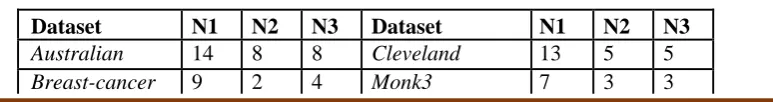
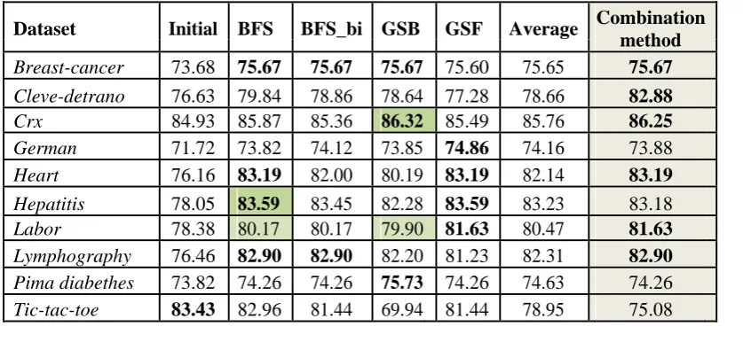
The exactness esteems acquired by the different strategies are introduced in Table 6, while the quantity of characteristics chosen by every strategy is shown in Table.7. As the outcomes demonstrate, an individual strategy can accomplish the best exactness on a dataset and the most noticeably bad on an alternate dataset, while the blend technique dependably yields better execution than the most noticeably bad individual strategy.

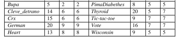
Table 5 – Number of attributes selected

Dataset N1 N2 N3 Dataset N1 N2 N3

Australian 14 8 8 Cleveland 13 5 5

(21)

Bupa 5 2 2 PimaDiabethes 8 5 5

Cleve_detrano 14 6 6 Thyroid 20 5 7

Crx 15 6 6 Tic-tac-toe 9 7 7

German 20 9 9 Vote 16 7 7

Heart 13 8 8 Wisconsin 9 5 5

N1 = Number of initial attributes in the dataset (without the class attribute); N2 = Number of attributes selected by the best wrapper method; N3 = Number of attributes selected by the wrapper which uses the best classifier (the classifier which achieved the best accuracy on the original dataset)

Table 6 – First and second best accuracies obtained after feature selection

Dataset A1 A2 A3 RI2 (%)

Australian 86.26 87.58 87.43 1.36

Breast-cancer 75.03 76.10 75.67 0.85

Bupa 63.1 65.17 64.8 2.69

Cleve_detrano 83.73 85.74 84.88 1.37

Crx 84.93 87.51 86.68 2.06

German 75.16 75.72 75.56 0.53

Heart 83.13 85.48 85.33 2.65

Cleveland 56.54 60.71 60.49 6.99

Monk3 98.91 98.92 98.92 0.01

PimaDiabethes 75.75 77.58 77.06 1.73

Thyroid 99.45 99.28 99.27 -0.18

Tic-tac-toe 83.43 83.47 83.47 0.05

Vote 96.22 96.73 96.71 0.51

Wisconsin 96.24 96.48 96.32 0.08

A1 = initial accuracy for the best classifier; A2 = Accuracy for the best wrapper method; A3 = Accuracy for the second best wrapper method; RI2 = Relative improvement for the second best wrapper method

Likewise, its execution is like the normal of the individual strategies, and in a few cases it accomplishes the best, or near the best execution (6

(22)

individual techniques and the mix strategy (at p=0.05). Additionally, with the exception of the GSF-based wrapper, there is a factual distinction between the execution of the individual techniques and the underlying execution, and furthermore between the blend strategy and the underlying execution. The dependability of the determination is along these lines accomplished, in this manner lessening the danger of choosing a wrong strategy in another issue.

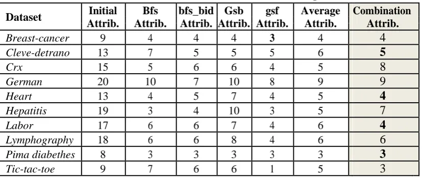
The diminishment in the quantity of qualities delivered by the mix strategy is likewise

noteworthy – like the normal lessening accomplished by the individual era methodologies. The relative lessening to the underlying trait set is of ~62%.

In this way, the mix technique gives a right evaluation of the normal execution change by means of highlight determination, by building up a pattern execution level for the investigated dataset and order strategy.

Table 7 – J4.8 accuracies on attribute subsets resulted from wrapper subset selection with various search strategies

Dataset Initial BFS BFS_bi GSB GSF Average Combination

method

Breast-cancer 73.68 75.67 75.67 75.67

75.60 75.65

75.67

Cleve-detrano 76.63 79.84 78.86 78.64

77.28 78.66

82.88

Crx 84.93 85.87 85.36 86.32 85.49 85.76 86.25

German 71.72 73.82 74.12 73.85

74.86 74.16

73.88

Heart 76.16 83.19 82.00 80.19

83.19 82.14

83.19

Hepatitis 78.05

83.59

83.45 82.28

83.59 83.23

83.18

Labor 78.38 80.17 80.17 79.90 81.63 80.47 81.63

Lymphography 76.46 82.90 82.90 82.20

81.23 82.31

82.90

Pima diabethes 73.82 74.26 74.26 75.73

74.26 74.63

74.26

(23)

Table 8 – Size of attribute subsets resulted from wrapper subset selection with various search strategies

Dataset Initial Bfs bfs_bid Gsb gsf Average Combination Attrib. Attrib. Attrib. Attrib. Attrib. Attrib. Attrib.

Breast-cancer 9 4 4 4 3 4

4

Cleve-detrano 13 7 5 5 5 6

5

Crx 15 5 6 6 4 5

8

German 20 10 7 10 8 9

9

Heart 13 4 5 7 4 5

4

Hepatitis 19 3 4 10 3 5

7

Labor 17 6 6 7 4 6

4

Lymphography 18 6 6 8 4 6

6

Pima diabethes 8 3 3 3 3 3

3

Tic-tac-toe 9 7 6 6 1 5

3

Conclusions on Feature Selection

Among the numerous conceivable favorable circumstances of highlight determination, maybe the most vital is enhancing the arrangement execution. All component determination strategies can be displayed as a mix of three stages: era, assessment and approval. The diverse options accessible for accomplishing each progression accommodate a wide range of highlight determination techniques. Be that as it may, much the same as on account of learning calculations, there is no all around best component choice technique. With the end goal of execution change, wrappers give the most fitting technique. A unique commitment exhibited in this thesis is the orderly investigation and the recognizable proof of the most encouraging blends of scan techniques for era,

and classifiers for assessment and approval, with

the end goal that the execution (i.e. the precision) increment is ensured. As the trial comes about demonstrate, wrappers can simply enhance the execution of classifiers. By and large, the classifier which at first accomplished the most astounding exactness keeps up its superior after element choice (first or second best execution). This implies once a dataset has been at first evaluated and a specific learning plan has been

chosen as being suitable, that plan will keep up its execution all through the mining procedure. Likewise, for all the datasets considered, the second best execution after element choice still yields noteworthy enhancements over the underlying classifier, which demonstrates the need for such a stage.

(24)

exactness in the majority of the cases. The wrapper _/JNP/JNP accomplishes the most noteworthy upgrades with respect to the underlying precision (up to 11%). The quantity of characteristics is impressively lessened (more than half), which brings about speedier preparing, yet another favorable position of property choice.

In the endeavor to diminish the predisposition presented by the inquiry techniques utilized as a part of the era methodology and enhance the dependability of highlight choice, without expanding its multifaceted nature, a unique mix strategy has been proposed, which chooses the most suitable qualities by applying a worldwide choice system on the characteristic subsets chose independently by the hunt strategies. Eager strategies have been considered for blend, since they give great quality arrangements moderately quick.

The assessments performed on the recently proposed strategy have affirmed that the technique accomplishes preferred strength over individual component choice performed by means of various pursuit strategies, while keeping the high decrease level. The technique can be utilized for introductory issue evaluation, to set up a gauge execution for highlight choice.

The original combination method and the analysis presented in this chapter have been acknowledged by the research community through the publication of 2 research papers in the proceedings of

renowned international conferences.

Joining Pre-processing Steps: A Methodology

Regardless of the possibility that critical endeavors

have been directed to create techniques which handle deficient information or perform highlight choice, with outstanding accomplishments in both fields autonomously, as far as anyone is concerned there hasn't been any endeavor to address the two issues in a joined way. This is what is proposed in this part – a joint component determination – information ascription pre-preparing philosophy.

A Joint Feature Selection – Data

Imputation Methodology

The oddity of our procedure comprises in the improvement of the information ascription venture with data given by the quality determination step. It considers the pre-preparing movement as a homogeneous assignment, joining the two once free strides:

• attribute determination • data attribution

(25)

i.e. just the estimations of the qualities which are important for the trait being attributed are utilized while deciding the substitution esteem. The strategy forces neither the procedure for quality choice, nor the information attribution system. In any case, an ascription system in light of regulated learning strategies ought to be utilized, keeping in mind the end goal to make utilization of the chose properties.

There are two variations of the technique. One performs information ascription first and afterward property subset determination, and the second which utilizes the invert arrange for the two. In this manner, we utilize the accompanying shortened forms:

• F – the first property set in the preparation set

• CT – subset of finish preparing cases

• ITj – subset of preparing occurrences with incentive for Xj missing

• AOSj – the prescient quality subset for Xj

• COS – the prescient quality subset for the class Y

FSAfterI

In the FSAfterI variant of the strategy, each trait Xj

with the exception of the class is considered. On the off chance that there are any occasions in the preparation set with obscure esteems for the present trait, the philosophy considers the characteristic for ascription. CT speaks to a subset of finish examples. For each characteristic Xj thus, a subset containing the inadequate cases regarding the property is extricated. The entire subset, CT, is utilized to fabricate the ascription display for thedeficient part, as portrayed further: the component subset prescient for quality Xj, AOSj, is separated from the total preparing subset. At that point, a model is worked for quality Xj utilizing the entire occasions subset and the components in AOSj. Utilizing this model, the swap esteems for the

fragmented examples are processed and credited in the underlying preparing set. Accordingly, the preparation set winds up plainly total in Xj. After every one of the traits have been viewed as, all examples in the preparation set are finished. Now, include choice is connected on the preparation set to decide the class-prescient element subset, COS. The projection of the preparation set on COS is the consequence of the technique.

(26)

FSAfterI

CT = extract_complete(T) T’ = T

For each attribute Xj

AOSj = fSelect(F – {Xj}



{Y}, CT, Xj)

T’ = Impute(prAOSjT’, Xj)

COS = fSelect(F,T’,Y)

Tresult = prCOST’

FSBeforeI

The second form of the proposed procedure, FSBeforeI, considers the two stages backward request. It does exclude any predisposition in the class-ideal quality determination stage, since the operation is performed before the ascription stage. [16] For deciding AOSj the first list of capabilities F and the class Y are utilized. In this manner we guarantee that all the significant traits for Xj are utilized to manufacture the ascription display. For

performing highlight choice, in both the era of COS and AOSj, k-overlay cross-approval is utilized, and the traits which are "better" on the normal are chosen. The strategy for evaluating "better" on the normal relies on upon the component determination technique utilized: positioning strategies yield normal legitimacy/rank measures, while different techniques may demonstrate a rate relating to the quantity of folds in which the characteristic has been chosen. In view of this data, the prescient subset can be concluded.

Experimental Evaluation

We have played out a few assessments with various usage of the consolidated philosophy, executed inside the WEKA structure. Beginning trials have been led on 14 benchmark datasets, gotten from the UCI vault. The ebb and flow assessments have been led on the accompanying complete UCI datasets: Bupa Liver Disorders, Cleveland Heart Disease, and Pima Indian Diabetes (depicted in Appendix A, table A.1).

The accompanying specializations of the approach have been considered:

 For quality determination (f): o ReliefF

 CFS – Correlation-based Feature Selection Wrapper

 For information attribution (i):

(27)

as IBk)

For assessing the execution (c): the normal characterization exactness figured utilizing 10 trials of a stratified 10-overlap cross approval for:

 J4.8

 Naïve Bayes (NB)

The hunt technique (era system) utilized in the quality determination is best-first pursuit. The prescient characteristic subset is acquired by means of 10-crease cross approval. For ascription with kNN, k has been set to 5. We have utilized the accompanying assessment system:

• Incompleteness has been reenacted, at various levels, utilizing the methodology depicted in segment

• In every trial of a stratified 10-crease

cross-approval, for each quality Ai in the trial preparing set (aside from the class) fluctuate the rate of inadequacy. At that point apply the pre-preparing procedure, in its present specialization, to acquire the preprocessed trial preparing set. At last, form a model from the adjusted preparing set, utilizing an arrangement calculation, and gauge its exactness utilizing the trial testing set.

• In expansion, for each quality Ai, the normal order precision has been assessed for

various renditions of the preparation set: finish, inadequate, credited and pre-handled through element determination.

The assessments endeavor to approve experimentally the accompanying explanations: the blend is more productive than the individual strides it joins, and the specializations of the mix are steady over the characteristics of a dataset – a similar specialization is distinguished just like the best for all the noteworthy qualities. By huge property we mean the traits which are always chosen by various element choice strategies. These are the characteristics that will impact the most the nature of the educated model.

(28)

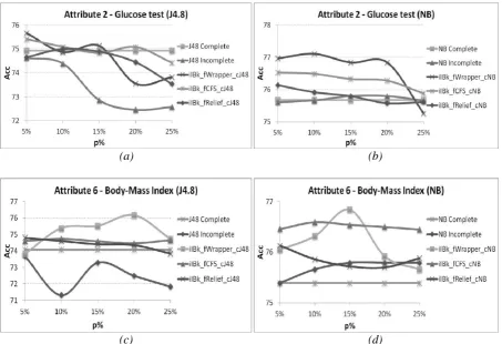
specializations for J4.8 (1-2% outright change accomplished by the CFS specializations, 1-3% by the wrapper up to 1% by the ReliefF based specializations). Be that as it may, NB is by all accounts more effective on the inadequate dataset, and the pre-preparing philosophy can't, for the most part, lift J4.8's exactness over NB's level (except for the wrapper based specialization). In this manner, specializations for NB ought to be considered here also. For the Cleveland dataset, the most huge changes are acquired by specializations for J4.8 (3-4%

accomplished by the CFS based specialization). In any case, the ReliefF specializations for NB yields the most astounding exactness levels: ~58% for both qualities broke down, rather than ~56% - the precision gotten by NB on the deficient renditions of the dataset, and ~56-56.5% - the precision acquired by the best specialization for J4.8 (utilizing CFS). The outcomes exhibited so far have demonstrated that we can play out the choice of the learning calculation before performing pre-handling with the proposed approach.

(a) (b)

(c) (d)

(29)

accuracy on the incomplete dataset, for attributes strongly correlated with the class, Pima dataset

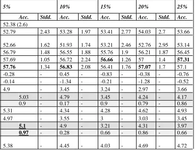
In the accompanying, we display a similar examination for the grouping execution on various variants of the preparation set, gotten through a few pre-handling procedures: ascription, characteristic choice and the consolidated strategy (both FSAfterI and FSBeforeI). Additionally, the order execution on the entire and p% fragmented datasets is accounted for. Tables 1-2 present the exactness

levels gotten for two huge traits of the Cleveland dataset. The specialization considered for the consolidated system utilizes CFS for trait choice. In both cases, the two variants of the joined technique yield preferred grouping exactnesses over the deficient dataset (up to 5% total increment). A reasonable change can be seen over the attribution step additionally (up to 5% supreme increment, the lines in dull dim shading in the tables). The

execution of highlight choice methodologies is like that of our proposed approach on this dataset.

Conclusions

There exist a progression of pre-handling assignments and related methods which concentrate on setting up the crude information for the mining step. In any case, every strategy concentrates on a solitary part of the information, and there is no data trade between free pre-handling steps. This part displays another approach for pre-handling, which

joins two some time ago free pre-preparing steps: information attribution and highlight determination.

The technique expressly performs trait determination for the information ascription stage. Two formal variants of the proposed technique have been presented: FSAfterI and FSBeforeI. The two contrast in the request of the two periods of the philosophy: the main performs information ascription first and afterward chooses the class-ideal element subset, while the second considers the invert arrange. FSBeforeI ought to be favored, since it doesn't present any ascription predisposition in the element determination stage.

(30)

addition, specializations utilizing CFS for quality determination and NB for the last characterization have dependably yielded higher exactness levels when contrasted with the precision on the deficient information. Likewise, the blend turns out to be better than the information ascription and trait determination assignments performed separately, which suggests it as a powerful approach for performing information pre-handling.

The outcomes have shown that, by and large, the change over the ascription undertaking is critical (a flat out increment in exactness of up to 5%). Concerning the correlation with the individual trait choice undertaking, much of the time the execution of the joined approach is better than that of the quality determination step (supreme change of up to 1%). In the special case cases, highlight determination yields the most astounding execution of the various methodologies.

The first information pre-preparing technique proposed in this part is the consequence of research bolstered by PNII give no.12080/2008: SEArCH – Adaptive E-Learning Systems utilizing Concept Maps. The proposed strategy has been acknowledged by the examination group through the distribution of two research papers in the procedures of prestigious global meetings:

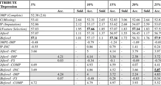
In the following, we present a comparative analysis

for the classification performance on different versions of the training set, obtained through several pre-processing strategies: imputation, attribute selection and the combined methodology (both FSAfterI and FSBeforeI). Also, the classification performance on the complete and p% incomplete datasets is reported. Tables 1-2 present the accuracy levels obtained for two significant attributes of the Cleveland dataset. The specialization considered for the combined methodology employs CFS for attribute selection. In both cases, the two versions of the combined

(31)

Table 9 : The average accuracy (and standard deviation) obtained by J4.8 on different versions of the training set and d for attribute STDepression, Cleveland dataset (specialization iIBk_fCfsSubsetEval_cJ)

ATTRIBUTE

5% 10% 15% 20% 25%

STDepression

Acc. Stdd. Acc. Stdd. Acc. Stdd. Acc. Stdd. Acc.

COMP (Complete) 52.38 (2.6)

INC(Missing) 53.41 2.64 52.31

2.65 52.83 3.06 52.66 2.64 52.83

IMP (Imputation) 52.86 2.12 53.17

2.17 53.62 2.68 54.07 2.59 53.07

FS(Feature Selection) 57.03 1.95 57.66 1.85 57.07 1.83 57.14 1.83 57.55

FSAfterI 57.07 1.11 57.31 1.37 56.97 1.55 56.45 1.17 56.79

FSBeforeI 57.1 1.01 57.17 1.1 57.34 1.72 56.31 1.76 57.9

COMPL-IMP -0.48 - -0.79 - -1.24 - -1.69 - -0.69

IMP-INC -0.55 - 0.86 - 0.79 - 1.41 - 0.24

FSAfterI –INC 3.66 - 5 - 4.14 - 3.79 - 3.97

FSAfterI –IMP 4.21

-

4.14

-

3.34

-

2.38

-

3.72

FSAfterI –FS 0.03 - -0.34 - -0.1 - -0.69

- -0.76

FSAfterI –COMP 4.69 - 4.93 - 4.59 - 4.07 - 4.41

FSBeforeI –INC 3.69 - 4.86

- 4.52

- 3.66

- 5.07

FSBeforeI –IMP 4.24

-

4

-

3.72

-

2.24

-

4.83

FSBeforeI –FS 0.07 - -0.48 - 0.28 - -0.83

- 0.34

(32)

Table 5.2 Table-10 : The average accuracy (and standard deviation) obtained by J4.8 on different versions of the training set and d for attribute Thal, Cleveland dataset (specialization

iIBk_fCfsSubsetEval_cJ48)

REFERENCES

1. [Fan00] Fan W., Stolfo S., Zhang J. and Chan P. (2000). AdaCost: Misclassification cost-sensitive boosting. Proceedings of the 16th _{International Conference on Machine}

Learning, pp. 97–105.

2. [Far09] Farid D.M., Darmont J., Harbi N., Hoa N.H., Rahman M.Z. (2009). Adaptive

Network Intrusion Detection Learning: Attribute Selection and Classification.

WorldAcademy of Science, Engineering and Technology 60. [Faw97] Fawcett T. and Provost F.J. (1997). Adaptive Fraud Detection. Data Mining and Knowledge Discovery, 1(3), pp. 291-316.

3. [Faw06] Fawcett T. (2006). An introduction to ATTRIBUTE

5% 10% 15% 20% 25%

Thal

Acc. Stdd. Acc. Stdd. Acc. Stdd. Acc. Stdd. Acc.

COMP (Complet 52.38 (2.6)

INC(Missing) 52.79 2.43 53.28 1.97 53.41 2.77 54.03 2.7 53.66

IMP

(Imputation) 52.66 1.62 51.93 1.74 53.21 2.46 52.76 2.95 53.14

FS(Feature Sele 56.79 1.48 56.55 1.88 55.76 1.9 56.21 1.87 56.45

FSAfterI 57.69 1.05 56.72 2.24 56.66 1.26 57 1.4 57.31

FSBeforeI 57.76 1.34 56.83 2.08 56.41 1.76 57.07 1.7 57.1

COMPL-IMP -0.28 - 0.45 - -0.83 - -0.38 - -0.76

IMP-INC -0.14 - -1.34 - -0.21 - -1.28 - -0.52

FSAfterI –INC 4.9 - 3.45

- 3.24

- 2.97

- 3.66

FSAfterI –IMP

5.03

-

4.79

-

3.45

-

4.24

-

4.17

FSAfterI –FS 0.9 - 0.17 - 0.9 - 0.79 - 0.86

FSAfterI –COMP 5.31 - 4.34 - 4.28 - 4.62 - 4.93

FSBeforeI –INC 4.97 - 3.55

- 3 - 3.03

- 3.45

FSBeforeI –IMP 5.1

-

4.9

-

3.21

-

4.31

-

3.97

FSBeforeI –FS 0.97 - 0.28 - 0.66 - 0.86 - 0.66

(33)

4. ROC analysis. Pattern Recognition Letters, 27, 861–874.

5. [Fay96] Fayyad U.M., Piatetsky-Shapiro G. and Smyth P. (1996). From Data Mining to Knowledge Discovery in Databases. Artificial Intelligence Magazine, 17(3): 37-54.

6. [Fei11] Feier M., Lemnaru C. and Potolea R. (2011). Solving NP-Complete Problems on the CUDA Architecture using Genetic Algorithms. In Proceedings ofISPDC 2011, pp. 278-

7. [Fir09] Firte A.A., Vidrighin B.C. and Cenan C. (2009). Intelligent component foradaptive E- learning systems. Proceedings of the IEEE 5th

International Conference on Intelligent Computer Communication and Processing. 27-29 August 2009, Cluj-Napoca, Romania. pp. 35-38.

8. [Fir10] Firte L., Lemnaru C. and Potolea R. (2010). Spam detection filter using KNN algorithm and resampling. Proceedings of the 2010 IEEE 6th _{International} _{Conference on}

Intelligent Computer Communication and Processing, pp.27-33.

9. [Fre97] Freund Y. and Shapire R. (1997). A decision-theoretic generalization of on-line learning and an application to boosting. Journal

of Computer and System Sciences, 55(1):119– 139.

10. [Gar09] García S. and Herrera F. (2009). Evolutionary Undersampling for Classification with Imbalanced Datasets: Proposals and Taxonomy. EvolutionaryComputation, Vol. 17, No. 3. pp. 275-306.

11. [Ged03] Gediga G. and Duntsch I. (2003). Maximum consistency of incomplete data via noninvasive imputation. Artificial intelligence Review, vol. 19, pp. 93-107.

12. Gen89] Gennari, J.H., Langley P. and Fisher D. (1989). Models of incremental concept formation. Artificial Intelligence, 40, pp.11-61.

13. [Gog10] Gogoi P., Borah B., Bhattacharyya D.K., (2010). Anomaly Detection Analysis of Intrusion Data using Supervised & Unsupervised Approach. Journal of Convergence Information Technology, vol. 5, no. 1, pp. 95-110.

14. [Gre86] Grefenstette, J.J. (1986). Optimization of control parameters for genetic algorithms. IEEE Transactions on Systems, Man, and Cybernetics, 16, 122-128.

(34)

values in preterm birth data. International journal of intelligent systems, vol. 17, pp. 125-134.

16. [Grz05] Grzymala-Busse J.W., Stefanowski J. and Wilk S. (2005). A comparison of two approaches