Western University Western University
Scholarship@Western
Scholarship@Western
Electronic Thesis and Dissertation Repository
9-23-2015 12:00 AM
Computing in Algebraic Closures of Finite Fields
Computing in Algebraic Closures of Finite Fields
Javad Doliskani
The University of Western Ontario Supervisor
Eric Schost
The University of Western Ontario Joint Supervisor Jan Minac
The University of Western Ontario Graduate Program in Computer Science
A thesis submitted in partial fulfillment of the requirements for the degree in Doctor of Philosophy
© Javad Doliskani 2015
Follow this and additional works at: https://ir.lib.uwo.ca/etd Part of the Computer Sciences Commons
Recommended Citation Recommended Citation
Doliskani, Javad, "Computing in Algebraic Closures of Finite Fields" (2015). Electronic Thesis and Dissertation Repository. 3282.
https://ir.lib.uwo.ca/etd/3282
This Dissertation/Thesis is brought to you for free and open access by Scholarship@Western. It has been accepted for inclusion in Electronic Thesis and Dissertation Repository by an authorized administrator of
Western University
Scholarship@Western
Electronic Thesis and Dissertation Repository
Computing in Algebraic Closures of Finite Fields
Javad Doliskani
Supervisor Eric Schost
The University of Western Ontario
Follow this and additional works at:http://ir.lib.uwo.ca/etd Part of theComputer Sciences Commons
Computing in Algebraic Closures of
Finite Fields
(Thesis format: Integrated-Article)
Javad Doliskani
Department of Computer Science A thesis submitted in partial fulfillment
of the requirements for the degree of Doctor of Philosophy
The School of Graduate and Postdoctoral Studies The University of Western Ontario
London, Ontario, Canada
Abstract
We present algorithms to construct and perform computations in algebraic closures of finite fields. Inspired by algorithms for constructing irreducible polynomials, our approach for con-structing closures consists of two phases; First, extension towers of prime power degree are built, and then they are glued together using composita techniques. To be able to move elements around in the closure we give efficient algorithms for computing isomorphisms and embeddings. In most cases, our algorithms which are based on polynomial arithmetic, rather than linear algebra, have quasi-linear complexity.
Co-Authorship
This document is based on the following joint works with Éric Schost and Luca Defeo.
Chapter 2 Taking roots over high extensions of finite fields.Mathematics of Computation, 83(285), pp. 435-446, 2014.
Chapter 3 Computing in degree 2k-extensions of finite fields of odd characteristic. Des. Codes Cryptography, 74(3), pp. 559-569, 2015.
Chapter 4 Fast algorithms for`-adic towers over finite fields. In Proceedings of the 38th Interna-tional Symposium on Symbolic and Algebraic Computation (ISSAC’13). ACM, New York, NY, USA.
List of Tables
2.1 Some special cases for square roots . . . 12
3.1 Costs for computations inFqn, withn=2k. . . 23
3.2 Timings for lifting 2k-torsion . . . 31
List of Figures
1.1 Algebraic closure ofFq . . . 5
2.1 Our square root algorithm vs. Cipolla’s and Tonelli-Shanks’ algorithms. . . 18
2.2 Our algorithm vs. Kaltofen and Shoup’s algorithm. . . 19
3.1 The new square root algorithm vs. the one in[6] . . . 30
4.1 The`-adic towers overFq andK0. . . 36
4.2 The isogeny cycle ofE0. . . 43
4.3 Times for building 3-adic towers on top ofF2(left) andF5(right), in Magma (first three lines) and using our code. . . 48
5.1 Timings in seconds, p=5,n=m+1 . . . 66
Contents
1 Introduction 2
1.1 Notations . . . 2
1.2 Our approach . . . 4
Bibliography . . . 7
2 Taking Roots over High Extensions of Finite Fields 9 2.1 Introduction . . . 9
2.2 Previous work . . . 12
2.3 A new root extraction algorithm . . . 14
2.3.1 An auxiliary algorithm . . . 15
2.3.2 Takingt-th roots . . . 16
2.3.3 Experimental results . . . 18
Bibliography . . . 20
3 Computing in Degree2k-Extensions of Finite Fields of Odd Characteristic 22 3.1 Introduction . . . 22
3.2 Proof of the complexity statements . . . 24
3.2.1 Representing the fieldsLk . . . 25
3.2.2 Arithmetic operations . . . 26
3.2.3 Frobenius computation . . . 26
3.2.4 Trace, norm and quadratic residuosity test . . . 27
3.2.5 Taking square roots . . . 28
3.2.6 Computing embeddings . . . 29
3.3 Experiments . . . 30
Bibliography . . . 31
4 Fast Algorithms for`-adic Towers over Finite Fields 33 4.1 Introduction . . . 33
4.2 Quasi-cyclotomic towers . . . 35
4.2.1 FindingP0 . . . 37
4.2.2 Gm-type extensions . . . 37
4.2.3 Chebyshev-type extensions . . . 37
4.2.4 The general case . . . 38
4.3.1 Towers from algebraic tori . . . 40
4.3.2 Towers from elliptic curves . . . 43
4.4 Lifting and pushing . . . 45
4.4.1 Lifting . . . 45
4.4.2 Pushing . . . 46
4.5 Implementation . . . 47
Bibliography . . . 48
5 Fast arithmetic for the algebraic closure of finite fields 51 5.1 Introduction . . . 51
5.2 Preliminaries . . . 53
5.2.1 Polynomial multiplication and remainder . . . 53
5.2.2 Duality and the transposition principle . . . 54
5.3 Trace and duality . . . 55
5.4 Embedding and isomorphism . . . 57
5.4.1 Embedding and computingR. . . 58
5.4.2 Isomorphism . . . 60
5.5 The algebraic closure of
F
p . . . 635.6 Implementation . . . 65
Bibliography . . . 67
Conclusion 70 A Finite Fields 71 A.1 Basic properties . . . 72
A.2 Irreducible polynomials . . . 73
A.3 Traces and Norms . . . 75
Chapter 1
Introduction
The theory of finite fields has found much attention during recent decades, most notably due to developments in the branches of computer science such as cryptography, coding theory, switch-ing circuits, and combinatorics[18]. In applications, one almost always encounters finite fields that are extensions of the so-called prime fields. For example, in public-key cryptography, there are cryptosystems that are based on the group of points on an algebraic curve. To have a secure system one must go through the process of choosing a random secure curve. A good class of candidates for such curves are hyperelliptic curves. One of the efficient methods of choosing a secure hyperelliptic curve requires counting the number of points on the curve, which in turn requires building a large number of successive extensions over a small prime field[10, 11]. The natural need for extensions usually arises from the need for manipulating polynomials and their roots. Once the extension are built, the next step is to be able to move elements from one extension to the other. This is where algebraic closures come to the fore. From a computational point of view, an algebraic closure of a given field can be seen as a large enough finite extension that contains the roots of a given finite set of polynomials. Computation in algebraic closures has been considered by others, e.g. [24]and references therein. In this chapter, we briefly review some basic properties of finite fields, and discuss some notations on the running time complexities of some basic arithmetics over them. At the end, we give an overview of our computational approach to algebraic closures.
1.1 Notations
In this section, we give a very brief review of finite fields concepts and notations used in the subsequent chapters. For a more detailed preliminary on finites fields we refer the reader to Appendix A. Given a prime number p, we denote the prime finite field with p elements byFp.
The prime number p is called the characteristic of the field.
Irreducible polynomials. The univariate polynomial ring overFp is denoted byFp[X]. The
elements ofFp[x]are of the form f(X) =anXn+an−1Xn−1+· · ·+a0whereai∈Fp. The degree
otherwise it is calledirreducible. For a monic irreducible polynomialsf of degreenthe quotient
Fp[X]/〈f〉is a finite field extension ofFp of degreen. We usually denote such an extension by Fqwhere q= pn.
Operation complexities The nature of the algorithms presented in this document suggests an algebraic complexity model. This means we will count operations{+,−,×,÷}in a based field such asFp orFq. Consequently, we have to choose a representation for elements of field
exten-sions. For example, one could proceed implementing algorithms using normal basis represen-tation, in which case the complexity estimates are stated differently. However, we shall use the monomial basis representation, since in particular our implementations and result comparisons are based on systems such as NTL[23], Magma[3], and FLINT[12]. In the monomial repre-sentation, the finite field or even ring extension are represented by quotients. For example, the finite fieldFqn is represented byFq[X]/〈f〉where f is a monic irreducible polynomial of degree n inFq[X]. So an elementa∈Fqn is a polynomial of degree less thanninFq[X].
One of the most fundamental operations in all algebraic systems ispolynomial multiplication. We denote the upper bound for the cost of multiplying two polynomials of degreenbyM(n). This means for a given fieldK and two polynomials f,g ∈K[X]of degree n, f g can be computed usingM(n)multiplications inK. The best known upper bound forM(n)isO(nlog(n)log log(n))
[19, 6]. This is done using Fast Fourier Transform. The idea is to reduce the polynomial multi-plication to point-wise vector-vector multimulti-plication using an invertible change of representation. See[27, Chapter 8]for more details. We assume that M(n) is a super-linear function, i.e. not bounded by any linear function.
Another fundamental operation ismatrix multiplication. Given two square matrices of size n
over a fieldK we assume they can be multiplied usingO(nω)multiplications inK, whereω is called the linear algebra exponent. A naive implementation would giveω=3. A slightly better algorithm due to Strassen[25]gives a boundω≤2.81. The algorithm uses a divide and conquer approach to reduce the multiplication problem to sub-blocks of the given matrices. The smallest known bound isω≤2.37 due to Coppersmith and Winograd[7].
Given polynomials f,g,h ∈ K[X] of degree n, the modular composition problem is to com-pute f(g) modh. We denote the upper bound for modular composition byC(n). In a boolean complexity model, in which bit or word operation are counted, there is an algorithm due to Ked-laya and Umans[15, 26]that runs inO(n1+"log(p)1+o(1))operations. Since we do not follow a
boolean model, and there is still no competitive implementation of their algorithm that we know of, we opt for the well-known algorithm of Brent and Kung[5]. Their algorithm gives the bound
O(n(ω+1)/2). We can takeω≤2.37 using the Coppersmith and Winograd algorithm which gives C(n) =O(n1.69). There is the slightly better boundC(n) =O(n1.67)due to Pan[13], which uses
rectangular matrix multiplication.
Algebraic closures. A field extensionK ⊆Lis said to be algebraic if every elementa∈Lis a root of a monic polynomial inK[X]. A fieldKis algebraically closed ifL=K for every algebraic extension ofL. An algebraic closure of a fieldK, denoted byK, is an algebraically closed algebraic extension ofK.
Generally, we can define the compositum of a family{Fi}i∈I of subfields of Lto be the smallest
subfield ofLcontaining allFi. The compositum ofE,F is not defined unless we have embeddings of both fields into a common fieldL. Let m= [E:K]andn= [F :K]. We have the following diagram of extensions:
L
E F
E F
K
≤n ≤m
m n
From the diagram [E F : K] ≤ mn and m | [E F :K] and n |[E F : K]. So if gcd(m,n) = 1 then [E F :K] = mn. Therefore, if E,F are finite fieldsFpn,Fpm with gcd(m,n) =1 then the
compositumE F is the finite fieldFpmn. This allows us to define the algebraic closure ofFpas the
union
Fp= [
i≥1
Fpi.
1.2 Our approach
Let Fq be a finite field with q = pn a prime power. We divide the construction ofFq into two
major steps: building towers, and gluing towers. Let us explain what these mean. Let ` be a prime number, and let
Fq⊂Fq`⊂Fq`2 ⊂ · · ·
a sequence of extensions each of degree`. We call this an`-adic tower. Define the`-adic closure
ofFq to be the union
F(`)q = [
i≥0
Fq`i.
Assume we have build these towers for different prime`. Then we can glue them together to get the algebraic closure. By gluing here we mean computing composita. Figure 1.1 shows the above structure ofFq. The solid circles in the middle are the composita.
`-adic towers. LetFi =Fq`i be the leveli of the`-adic tower for an integeri >0. The goal is
to be able to compute inFiin quasi-linear time in the extension degree`i. For this we need first
to construct the tower, and then be able to move up and down to different levels of the tower efficiently.
Fq Fq2
Fq4
F(q2)
Fq3
Fq9
F(q3)
Fq5
Fq25
F(q5)
Fq`
Fq`2
F(q`)
Figure 1.1: Algebraic closure ofFq
to reduce the problem to root extraction in subfields using trace-like computations. For example, using our algorithm, the complexity of taking square roots inFq is an expectedO(M(n)log(p)+
C(n)log(n))operations inFp. Computing roots in finite fields was previously considered by
oth-ers like Cipolla [28] and Tonelli-Shanks [20]. Kaltofen and Shoup[14] give an Equal Degree Factorization (EDF) algorithm that can be used for computing roots.
The case`=2 of the`-adic towers, which is of particular interest, is treated separately in Chapter 3. Our algorithms presented there for construction of the tower and performing basic operations inside the tower are all quasi-linear time. The following table summarizes the complexities of our algorithms for some well-known operations for this case.
Operation Cost addition/subtraction O(n)
multiplication M(n) +O(n)
inversion O(M(n))
quadratic residuosity O(M(n) +log(q))
square root O(M(n)log(nq)) (expected) isomorphism O(n+log(n)log(q)) (expected)
Note the improvement of the square root complexity here compared to the one for general finite fields which has aC(n)term. Another special case of the`-adic towers is`= p, called the Artin-Schreier tower. The algorithms for this case were presented in[9].
Chapter 4 discusses the towers for a general`. The fieldFq`i can be represented by two natural
bases overFq. For a univariate representation of the formFq[Xi]/〈Qi〉, whereQi∈Fq[Xi]is a
monic irreducible polynomial of degree`i, we get the monomial basis
forFq`i overFq. Herexi is the residue class ofXimoduloQi. But we can also considerF q`i as a
degree`extension overFq`i−1, i.e. as a bivariate quotient
Fq[Xi−1,Xi]/〈Qi−1(Xi−1),Ti(Xi−1,Xi)〉
whereTiis a monic polynomial of degree`inXi, and of degree less than`i−1inX
i−1. This gives
the basis
Bi= (1, . . . ,xi`−i−11−1, . . . ,xi`−1, . . . ,xi`−i−11−1xi`−1).
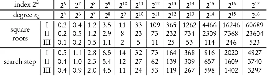
forFq`i overFq. The complexity of constructing the tower, which requires some initialization
and findingQi,Ti, is close to quasi-linear. Using the usual algorithms, basic operations like multi-plication and inversion inFq[Xi]/〈Qi〉are done using respectivelyO(M(`i))andO(M(`i)log(`i))
operations inFq. These are quasi-linear in the extension degree`i. Moving up and down in the
tower is done using repeated applications of two operations calledliftandpush. Lifting refers to the change of basis fromBi toUi while pushing is the inverse transformation. These operations are also very close to being quasi-linear. The following table summarizes our main complexity results.
Condition Initialization Qi,Ti Lift, push
q=1 mod` Oe(log(q)) O(`i) O(`i)
q=−1 mod` Oe(log(q)) O(`i) O(M(`i)log(`i))
− Oe(`2+M(`)log(q)) O(M(`i+1)M(`)log(`i)2) O(M(`i+1)M(`)log(`i))
4`≤q1/4 O˜
e(`log
5(q) +`3)(bit) O
e(`2+M(`)log(`q) +M(`i)log(`i)) O(M(`i)log(`i))
4`≤q1/4 O˜
e(`log
5(q))
(bit)+Oe(M(`)pqlog(q)) Oe(log(q) +M(`i)log(`i)) O(M(`i)log(`i))
The probabilistic complexities with expected running time are denoted by Oe( ). Also O˜e( ) indicates the additional omission of logarithmic factors. Although in some cases there are extra factors of`, we have achieved quasi-linear time in the degree of the extension`i in most of the
cases. Our algorithm for constructing towers are inspired by the previous works of Shoup[21, 22] and Lenstra/De Smit[16], and Couveignes/Lercier[8]. See the introduction of Chapter 4 for more details.
Composita. In Chapter 5, we discuss the composita of fields. LetFpm =Fp[x]/〈Qm(x)〉and Fpn =Fp[y]/〈Qn(y)〉be two finite fields whereQm(x)∈Fp[x]andQn(y)∈Fp[y]are irreducible
of comprime degreesm,n>1 respectively. Define thecomposed productofQm,Qnas
Qmn(z) = Y
1≤i≤m
1≤j≤n
(z−aibj)
where(ai)1≤i≤m and(bj)1≤j≤n are roots ofQmandQnin the algebraic closure ofFp. The
poly-nomialQmn is irreducible of degreemninFp[z], see[4]. The fieldFp[z]/〈Qmn(z)〉is the
com-positum ofFpm andFpn, and there exists embeddingsϕx,ϕy, and an isomorphismΦof the form ϕx: Fp[x]/〈Qm〉 → Fp[z]/〈Qmn〉,
ϕy: Fp[y]/〈Qn〉 → Fp[z]/〈Qmn〉, Φ: A=Fp[x,y]/〈Qm,Qn〉 → Fp[z]/〈Qmn〉
The goal is to computeϕx,ϕy, andΦandΦ−1efficiently. We present algorithms for computing
ϕxandϕy which run usingO(nM(m) +mM(n))operations inFp. Assuming thatm≤n,Φand Φ−1can be computed using eitherO(m2M(n))orO(M(mn)n1/2+M(m)n(ω+1)/2)operations in
Fp whereω is the linear algebra exponent. Therefore, computing embeddingsϕx,ϕy is
quasi-linear in mnwhile computing the isomorphismsΦ,Φ−1has an extra factor of morn. Previous
algorithms such as the ones presented in[2], and[17, 1]also compute embeddings of finite fields. They rely on linear algebra which results in complexities at least quadratic in the degree of the extensions.
Bibliography
[1] B. Allombert. Explicit computation of isomorphisms between finite fields. Finite Fields Appl., 8(3):332 – 342, 2002.
[2] W. Bosma, J. Cannon, and A. Steel. Lattices of compatibly embedded finite fields. J. Symb. Comput., 24(3-4):351–369, 1997.
[3] Wieb Bosma, John Cannon, and Catherine Playoust. The MAGMA algebra system I: the user language. J. Symbolic Comput., 24(3-4):235–265, 1997.
[4] J.V. Brawley and L. Carlitz. Irreducibles and the composed product for polynomials over a finite field. Discrete Mathematics, 65(2):115 – 139, 1987.
[5] R. P. Brent and H. T. Kung. Fast algorithms for manipulating formal power series. Journal of the Association for Computing Machinery, 25(4):581–595, 1978.
[6] D. G. Cantor and E. Kaltofen. On fast multiplication of polynomials over arbitrary alge-bras. Acta Informatica, 28(7):693–701, 1991.
[7] D. Coppersmith and S. Winograd. Matrix multiplication via arithmetic progressions. J. Symb. Comp, 9(3):251–280, 1990.
[8] Jean-Marc Couveignes and Reynald Lercier. Fast construction of irreducible polynomials over finite fields. To appear in the Israel Journal of Mathematics, July 2011.
[9] L. De Feo and É. Schost. Fast arithmetics in Artin-Schreier towers over finite fields. Journal of Symbolic Computation, 47(7):771–792, 2012.
[10] Luca De Feo. Fast algorithms for computing isogenies between ordinary elliptic curves in small characteristic. Journal of Number Theory, 131(5):873–893, May 2011.
[11] P. Gaudry and É. Schost. Point-counting in genus 2 over prime fields. J. Symbolic Comput., 47(4):368–400, 2012.
[13] X. Huang and V. Y. Pan. Fast rectangular matrix multiplication and applications. J. Com-plexity, 14(2):257–299, 1998.
[14] E. Kaltofen and V. Shoup. Fast polynomial factorization over high algebraic extensions of finite fields. InISSAC’97, pages 184–188. ACM, 1997.
[15] K. S. Kedlaya and C. Umans. Fast polynomial factorization and modular composition.
SIAM J. Computing, 40(6):1767–1802, 2011.
[16] Hendrick W. Lenstra and Bart De Smit. Standard models for finite fields: the definition, 2008.
[17] H. W. Lenstra Jr. Finding isomorphisms between finite fields. Math. Comp., 56(193):329– 347, 1991.
[18] Rudolf Lidl and Günter Pilz. Applied abstract algebra. Springer Science & Business Media, 2012.
[19] A. Schönhage and V. Strassen. Schnelle Multiplikation grosser Zahlen. Computing, 7:281– 292, 1971.
[20] D. Shanks. Five number-theoretic algorithms. InProceedings of the Second Manitoba Con-ference on Numerical Mathematics, pages 51–70, 1972.
[21] Victor Shoup. New algorithms for finding irreducible polynomials over finite fields. Math. Comp., 54:435–447, 1990.
[22] Victor Shoup. Fast construction of irreducible polynomials over finite fields. J. Symbolic Comput., 17(5):371–391, 1994.
[23] Victor Shoup. NTL: A library for doing number theory. http://www.shoup.net/ntl, 2003.
[24] Allan K. Steel. Computing with algebraically closed fields. Journal of Symbolic Computa-tion, 45(3):342 – 372, 2010.
[25] Volker Strassen. Gaussian elimination is not optimal. Numerische Mathematik, 13(4):354– 356, 1969.
[26] C. Umans. Fast polynomial factorization and modular composition in small characteristic. InSTOC, pages 481–490, 2008.
[27] J. von zur Gathen and J. Gerhard. Modern Computer Algebra. Cambridge University Press, 2003.
Chapter 2
Taking Roots over High Extensions of
Finite Fields
2.1 Introduction
Beside its intrinsic interest, computingm-th roots over finite fields (forman integer at least equal to 2) has found many applications in computer science. Our own interest comes from elliptic and hyperelliptic curve cryptography; there, square root computations show up in pairing-based cryptography[3]or point-counting problems[8].
Our result in this paper is a new algorithm for computing m-th roots in a degree n extension
Fq of the prime fieldFp, with p a prime. Our emphasis is on the case where p is thought to be
small, and the degreengrows. Roughly speaking, we reduce the problem tom-th root extraction in a lower degree extension ofFp (when m=2, we actually reduce the problem to square root
extraction overFp itself).
Our complexity model. It is possible to describe the algorithm in an abstract manner, indepen-dently of the choice of a basis ofFq overFp. However, to give concrete complexity estimates, we
have to decide which representation we use, the most usual choices being monomial and normal bases. We choose to use a monomial basis, since in particular our implementation is based on the library NTL[22], which uses this representation. Thus, the finite field Fq =Fpn is represented
asFp[X]/〈f〉, for some monic irreducible polynomialf ∈Fp[X]of degreen; elements ofFqare
represented as polynomials inFp[X]of degree less thann. We will briefly mention the normal
basis representation later on.
The costs of all algorithms are measured in number of operations +,×,÷in the base field Fp
(that is, we are using an algebraic complexity model) — at the end of this introduction, we discuss how our results can be stated in the boolean model, in light especially of results by Umans[25] and Kedlaya and Umans[13].
We shall denote upper bounds for the cost ofpolynomial multiplicationandmodular composition
by respectivelyM(n)andC(n). This means that over any fieldK, we can multiply polynomials
of degreeninK[X]inM(n)base field operations, and that we can compute f(g)modhinC(n)
Care super-linear functions, as in[26, Chapter 8], and thatM(n) =O(C(n)). In particular, since we work in the monomial basis, multiplications and inversions inFq can be done in respectively O(M(n))andO(M(n)log(n))operations inFp, see again[26].
The best known bound forM(n)isO(nlog(n)log log(n)), achieved by using Fast Fourier Trans-form[19, 5]. The most well-known bound forC(n)is O(n(ω+1)/2), due to Brent and Kung[4],
whereωis such that matrices of sizenover any fieldKcan be multiplied inO(nω)operations in K; this estimate assumes thatω >2, otherwise some logarithmic terms may appear. Using the
algorithm of Coppersmith and Winograd[6], we can takeω≤2.37 and thusC(n) =O(n1.69); an algorithm by Huang and Pan[10]actually achieves a slightly better exponent of 1.67, by means of rectangular matrix multiplication.
Main result. We will focus in this paper on the case of t-th root extraction, where t is a prime divisor ofq−1; the general case ofm-th root extraction, withmarbitrary, can easily be reduced to this case (see the discussion after Theorem 20).
The core of our algorithm is a reduction oft-th root extraction inFqtot-th root extraction in an
extension ofFpof smaller degree. Our algorithm is probabilistic of Las Vegas type, so its running
time is given as an expected number of operations. With this convention, our main result is the following.
Theorem 1. Let t be a prime factor of q −1, with q = pn, and let s be the order of p in
Z/tZ.
Given a ∈F∗q, one can decide if a is a t -th power in F∗q, and if so compute one of its t -th roots, by means of the following operations:
• an expected O(sM(n)log(p) +C(n)log(n))operations inFp; • a t -th root extraction inFps.
Thus, we replace t-th root extraction in a degree n extension by a t-th root extraction in an extension of degree s ≤ min(n,t). The extension degree s is the largest one for which t still divides ps−1, so iterating the process does not bring any improvement: thet-th root extraction
inFps must be dealt with by another algorithm. The smaller s is, the better.
A useful special case is t =2, that is, we are taking square roots; the assumption that t divides
q−1 is then satisfied for all odd primes p and alln. In this case, we have s =1, so the second step amounts to square root extraction inFp. Since this can be done inO(log(p))expected
oper-ations inFp, the total running time of the algorithm is an expectedO(M(n)log(p)+C(n)log(n))
operations inFp.
A previous algorithm by Kaltofen and Shoup[12]allows one to compute t-th roots in Fpn in
expected timeO((M(t)M(n)log(p) +tC(n) +C(t)M(n))log(n)); we discuss it further in the next section. This algorithm requires no assumption ont, so it can be used in our algorithm in the case
s >1, for t-th root extraction inFps. Then, its expected running time isO((M(t)M(s)log(p) + tC(s) +C(t)M(s))log(s)).
The strategy of using Theorem 20 to reduce fromFq toFps then using the Kaltofen-Shoup
our algorithm has advantages (as explained in the last section). For largert, the gap in our favor will increase for cases whens is small (such as whent divides p−1, corresponding to s =1). Finally, let us go back to the remark above, that for anym, one can reduce m-th root extraction ofa∈F∗q to computingt-th roots, witht dividingq−1; this is well known, see for instance[1,
Chapter 7.3]. We writem=uv with(v,q−1) =1 and t|q−1 for every prime divisort of u, and we assume thata is indeed anm-th power.
• We first compute the v-th root a0 of a asa0 =av−1modq−1 by computing the inverse` of
v modq−1, and computing an`-th power inFq. This takesO(nM(n)log(p))operations
inFp.
• Let u=Qdi=1mαi
i be the prime factorization of u, which we assume is given to us. Then,
fork=1, . . . ,α1, we compute anm1-th rootak ofak−1using Theorem 20, so thataα 1 is an mα1
1 -th root ofa0.
One should be careful in the choice of the m1-th roots (which are not unique), so as to ensure that eachak is indeed anu/mi
1-th power: if the givenakis not such a power, we can
multiply it by am1-th root of unity until we find a suitable one. The root of unity can be found by the algorithm of Theorem 20.
Once we knowaα
1, the same process can be applied to compute an m
α2
2 -th root ofaα1, and
so on.
The first step, taking a root of orderv, may actually be the bottleneck of this scheme. Whenv
is small compared ton, it may be better to use here as well the algorithm by Kaltofen and Shoup mentioned above.
In a boolean model. In our algebraic model, whenn grows, the bottleneck of our algorithm (or of the Kaltofen-Shoup algorithm) is modular composition, since there is currently no known algorithm with cost quasi-linear inn.
If we analyze running times in a boolean model (counting bit or word operations), much better can be done: Kedlaya and Umans[13], following previous work by Umans[25], give an algo-rithm with a boolean cost that grows liken1+"log(p)1+o(1)for modular composition in degreen
overFp, for any given" >0. They also show that minimal polynomial of elements ofFq=Fpn
can be computed for the same cost.
The algorithms of the following sections can be analyzed in the boolean model without difficulty (for definiteness, over a boolean RAM with logarithmic access cost — the Kedlaya-Umans algo-rithm uses table lookup in large tables). The only differences are in the cost of modular composi-tion overFp, as well as minimal polynomial computation inFq, for which we use the results by
Kedlaya and Umans. Using the fact that arithmetic inFpcan be done in boolean time log(p)1+o(1),
the running time reported in Theorem 20 then becomesO(sM(n)log(p)2+o(1)+n1+"log(p)1+o(1))
bit operations, for any" >0; this admits the upper boundO(s n1+"log(p)2+o(1)). With respect to
the extension degreen, this is close to being linear time.
Organization of the chapter. The next section reviews and discusses known algorithms; Sec-tion 2.3 gives the details of the root extracSec-tion algorithm and some experimental results. In all the paper,(F∗q)t denotes the set of t-th powers inF∗q.
Acknowledgments. We thank NSERC and the Canada Research Chairs program for financial support. We also thank the referee for very helpful remarks.
2.2 Previous work
Lettbe a prime factor ofq−1. In the rest of this section, we discuss previous algorithms fort-th root extraction, with a special focus on the case t =2 (square roots), which has attracted most attention in the literature. Note that our assumptions exclude the case of pth root extraction in characteristic p.
We shall see in Section 2.3 that given a prime t as above, the cost of testing for t-th power is always dominated by the t-th root extraction; thus, for an inputa ∈F∗q, we always assume that a∈(F∗q)t.
All algorithms discussed below rely on some form of exponentiation inFq, or in an extension of Fq, with exponents that grow linearly withq. As a result, a direct implementation using binary
powering usesO(log(q))multiplications inFq, that is,O(nM(n)log(p))operations inFp. Even
using fast multiplication, this is quadratic inn; alternative techniques should be used to perform the exponentiation, when possible.
Some special cases of square root computation. IfG is a group with an odd order s, then the mapping f :G→G, f(a) =a2is an automorphism ofG; hence, every elementa∈Ghas a
unique square root, which isa(s+1)/2. Thus, ifq≡3(mod 4), the square root of anya∈(F∗q)2is a(q+1)/4; this is because(
F∗q)2is a group of odd order(q−1)/2.
More complex schemes allow one to compute square roots for some increasingly restricted classes of prime powersq. The following table summarizes results known to us; in each case, the algo-rithm usesO(1)exponentiations andO(1)additions/multiplications inFq. The table indicates
what exponents are used in the exponentiations.
Table 2.1: Some special cases for square roots Algorithm q exponent
folklore 3(mod 4) (q+1)/4 Atkin 5(mod 8) (q−5)/8
Müller[15] 9 (mod 16) (q−1)/4 and(q−9)/16 Konget al.[14] 9 (mod 16) (q−9)/8 and(q−9)/16
in the literature, for example to cube roots in the case where q =7(mod 9)[17], with similar running times.
Cipolla’s square root algorithm. To compute the square root ofa∈(F∗q)2, Cipolla’s algorithm
uses an element b inFq such that b2−4a is not a square inFq. Then, the polynomial f(Y) = Y2−b Y+a is irreducible over
Fq, henceK=Fq[Y]/〈f〉is a field. Let y be the residue class
ofY modulo〈f〉. Since f is the minimal polynomial of y overFq,NK/Fq(y) =a, ensuring that p
a=Y(q+1)/2mod(Y2−b Y+a).
Finding a quadratic nonresidue of the form b2−4a by choosing a random b ∈
Fq requires an
expectedO(1)attempts[1, page 158]. The quadratic residue test, and the norm computation take
O(M(n)log(n) +log(p))andO(nM(n)log(p))multiplications inFprespectively. Therefore, the
cost of the algorithm is an expectedO(nM(n)log(p))operations inFp.
Algorithms extending Cipolla’s to the computation oft-th roots inFp, wheretis a prime factor
of p−1, are in[27, 28, 16].
The Tonelli-Shanks algorithm. We will describe the algorithm in the case of square roots, al-though the ideas extend to higher orders. Tonelli’s algorithm[23]and Shanks’ improvement[20] use discrete logarithms to reduce the problem to a subgroup ofF∗q of odd order. Letq−1=2r`
with(`, 2) =1 and letH be the unique subgroup ofF∗q of order`. Assume we find a quadratic
nonresidue g ∈ F∗q; then, the square root of a ∈ F∗q can be computed as follows: we can
ex-press a as gsh ∈ gsH by solving a discrete logarithm in
F∗q/H; s is necessarily even, so that p
a=gs/2h(`+1)/2.
According to [18], the discrete logarithm requires O(r2M(n)) multiplications in
Fp; all other
steps take O(nM(n)log(p)) operations in Fp. Hence, the expected running time of the
algo-rithm is O((r2+nlog(p))M(n)) operations in
Fp. Thus, the efficiency of this algorithm
de-pends on the structure of F∗q: there exists an infinite sequence of primes for which the cost is O(n2M(n)log(p)2), see[24]. An extension to the computation of cube roots modulo pis in[17],
with a similar cost analysis.
Improving the exponentiation. All algorithms seen before use at bestO(nM(n)log(p)) op-erations inFp, because of the exponentiation. Using ideas going back to[11], Barretoet al.[3]
observed that for some of the cases seen above, the exponentiation can be improved, giving a cost subquadratic inn.
For instance, when taking square roots withq =3 (mod 4), the exponentiationa(q+1)/4can be
reduced to computinga1+u+···+u(n−3)/2
, with u = p2, plus two (cheap) exponentiations with
expo-nents p(p−1)and(p+1)/4. The special form of the exponent 1+u+· · ·+u(n−3)/2makes it
possible to apply a binary powering approach, involvingO(log(n))multiplications and exponen-tiations, with exponents that are powers of p.
Further examples for square roots are discussed in[14, 9], covering the entries of Table 2.1. These references assume a normal basis representation; using (as we do) the monomial basis and mod-ular composition techniques (which will be explained in the next section), the costs become
p−1, such that t2does not divide p−1, and if gcd(n,t) =1, then t-th root extraction can be
done usingO(tM(n)log(p) +C(n)log(n))operations inFp.
Kaltofen and Shoup’s algorithm. Finally, we mention what is, as far as we know, the only algorithm achieving an expected subquadratic running time inn(using the monomial basis rep-resentation), without any assumption on p.
Consider a factor t of q−1. To compute a t-th root ofa ∈(F∗q)t, the idea is simply to factor Yt−a∈
Fq[Y]using polynomial factorization techniques. Since we know thatais at-th power,
this polynomial splits into linear factors, so we can use an Equal Degree Factorization (EDF) algorithm.
A specialized EDF algorithm, dedicated to the case of high-degree extension of a given base field, was proposed by Kaltofen and Shoup [12]. It mainly reduces to the computation of a trace-like quantity b +bp+· · ·+bpn−1, where b is a random element in Fq[Y]/〈Yt−a〉. Using a
binary powering technique similar to the one of the previous paragraph, this results in an ex-pected running time of O((M(t)M(n)log(p) +tC(n) +C(t)M(n))log(n)) operations inFp;
re-mark that this estimate is faster than what is stated in[12]by a factor log(t), since here we only need one root, instead of the whole factorization. In the particular case t = 2, this becomes
O((M(n)log(p) +C(n))log(n)). This achieves a running time subquadratic inn.
This idea actually allows one to compute at-th root, for arbitraryt: starting from the polynomial
Yt−a, we apply the above algorithm to gcd(Yt−a,Yq−Y); computingYq moduloYt−acan
be done by the same binary powering techniques.
2.3 A new root extraction algorithm
In this section, we focus ont-th root extraction inFq, fort a prime dividingq−1 (as we saw in
Section 3.1,m-th root extraction, for an integerm≥2, reduces to takingt-th roots, wheret is a prime factor ofmdividingq−1).
The algorithm we present uses the traceFq→Fq0, for some subfieldFq0⊂Fq to reducet-th root
extraction inFqtot-th root extraction inFq0. We assume as before that the fieldFqis represented
by a quotientFp[X]/〈f〉, with f(X)∈Fp[X]a monic irreducible polynomial of degreen. We
letx be the residue class ofX modulo〈f〉.
Since we will handle bothFq andFq0, conversions may be needed. We recall that the minimal
polynomial g ∈Fp[Z]of an elementb ∈Fq can be computed inO(C(n) +M(n)log(n))
opera-tions inFp [21]. Then,Fq0=Fp[Z]/〈g〉is a subfield ofFq=Fp[X]/〈f〉; given r ∈Fq0, written
as a polynomial inZ, we obtain its representation on the monomial basis ofFq by means of a
2.3.1 An auxiliary algorithm
We first discuss a binary powering algorithm to solve the following problem. Starting fromλ∈ Fq, we are going to compute
αi(λ) =λ1+p s
+λ1+ps+p2s
+· · ·+λ1+ps+p2s+···+pi s
for given integers i,s >0. This question is similar to (but distinct from) some exponentiations and trace-like computations we discussed before; our solution will be a similar binary powering approach, which will performO(log(i)) multiplications and exponentiations by powers of p. Let
ξi=xp i s
, ζi(λ) =λps+p2s+···+pi s and δi(λ) =λps+λps+p2s+· · ·+λps+p2s+···+pi s, where all quantities are computed inFq, that is, modulo f; for simplicity, in this paragraph, we
will writeαi,ζi andδi. Note thatαi=λδi, and that we have the following relations:
ξ1=x
ps
, ζ1=λps, δ1=λps and
ξi= (
ξpi s/2
i/2 ifi is even
ξps
i−1 ifi is odd,
ζi= (
ζi/2ζ
pi s/2
i/2 ifi is even
ζ1ζ
ps
i−1 ifi is odd,
δi= (
δi/2+ζi/2δ
pi s/2
i/2 ifi is even
δi−1+ζi ifi is odd.
Because we are working in a monomial basis, computing exponentiations to powers of p is not a trivial task; we will perform them using the following modular composition technique from[7]. Take j ≥0 and r ∈Fq, and letRandΞj be the canonical preimages of respectively r andξj in Fp[X]; then, we have
rpj s =R(Ξj)mod f,
see for instance[26, Chapter 14.7]. We will simply write this as r(ξj), and note that it can be computed using one modular composition, in time C(n). These remarks give us the following recursive algorithm, where we assume thatξ1=xps andζ
1=λp
s
are already known.
Algorithm 1XiZetaDelta(λ,i,ξ1,ζ1)
Input: λ, a positive integeri,ξ1=xps
,ζ1=λps
Output: ξi,ζi,δi
1. ifi =1then
2. return ξ1,ζ1,ζ1
3. end if
4. j ← bi/2c
5. ξj,ζj,δj←XiZetaDelta(λ,j,ξ1,ζ1)
6. ξ2j←ξj(ξj)
7. ζ2j←ζj·ζj(ξj)
8. δ2j←δj+ζjδj(ξj)
10. return ξ2j,ζ2j,δ2j 11. end if
12. ξi←ξ2j(ξ1)
13. ζi←ζ1·ζ2j(ξ1)
14. δi←δ2j+ζi
15. return ξi,ζi,δi
We deduce the following algorithm for computingαi(λ).
Algorithm 2Alpha(λ,i)
Input: λ, a positive integeri
Output: αi
1. ξ1←xps
2. ζ1←λps
3. ξi,ζi,δi←XiZetaDelta(λ,i,ξ1,ζ1)
4. return λδi
Proposition 2. Algorithm 2 computesαi(λ)using O(C(n)log(i s)+M(n)log(p))operations inFp. Proof. To compute xps andλps we first compute xp andλp usingO(log(p))multiplications in Fq, and then doO(log(s))modular compositions modulo f. The depth of the recursion in
Al-gorithm 1 isO(log(i)); each recursive call involvesO(1)additions, multiplications and modular compositions modulo f, for a total time ofO(C(n))per recursive call.
As said before, the algorithm can also be implemented using a normal basis representation. Then, exponentiations to powers of p become trivial, but multiplication becomes more difficult. We leave these considerations to the reader.
2.3.2 Taking
t
-th roots
We will now give our root extraction algorithm. As said before, we now let t be a prime factor ofq−1, and we let s be the order of p inZ/tZ. Thens dividesn, sayn=s`.
We first explain how to test for t-th powers. Testing whether a ∈F∗q is a t-th power is
equiv-alent to testing whether a(q−1)/t = 1. Let ζ = a(ps−1)/t
; then a(q−1)/t = ζ1+ps+···+p(`−1)s
. Com-puting ζ requires O(sM(n)log(p)), and computing ζ1+ps+···+p(`−1)s
using Algorithm 1 requires
O(C(n)log(n)+M(n)log(p))operations inFp. Therefore, testing for at-th power takesO(C(n)log(n)+ sM(n)log(p))operations inFp.
In the particular case whentdividesp−1, we can actually do better: we havea(q−1)/t=res(f,a)(p−1)/t,
In any case, we can now assume that we are given a ∈(F∗q)t, with t-th root γ ∈Fq. Defining β=trF
q/Fq0(γ), where trFq/Fq0 :Fq→Fq0 is the trace linear form andq
0=ps, we have β= `−
1
X
i=0
γpi s
=γ(1+γps−1+γp2s−1+· · ·+γp(`−1)s−1)
=γ(1+a(ps−1)/t+a(p2s−1)/t+· · ·+a(p(`−1)s−1)/t). (2.1) Let b =1+a(ps−1)/t
+a(p2s−1)/t
+· · ·+a(p(`−1)s−1)/t
, so that Equation 3.3 givesβ=γb. Taking the t-th power in both sides results in the equationβt=abt over
Fq0. Since we knowa, and we
can computeb, we can thus determineβbyt-th root extraction inFq0. Then, if we assume that
b6=0 (or equivalently thatβ6=0), we deduceγ =βb−1; to resolve the issue thatβmay be zero,
we will replaceabya0=act, for a random elementc∈ F∗q.
Computing the t-th root ofa0bt in
Fq0 is done as follows. We first compute the minimal
poly-nomial g∈Fp[Z]ofa0bt, and letz be the residue class ofZ inFp[Z]/〈g〉. Then, we compute a t-th rootr ofz inFp[Z]/〈g〉, and embed r inFq. The computation ofr is done by a black-box t-th root extraction algorithm, denoted byr 7→r1/t.
It remains to explain how to compute b efficiently. Let λ = a(ps−1)/t; then, one verifies that b=1+λ+α`−2(λ), so we can use the algorithm of the previous subsection. Putting all together, we obtain the following algorithm
Algorithm 3t-th root inF∗q
Input: a∈(F∗q)t
Output: at-th root ofa 1. s ←the order of p inZ/tZ
2. `←n/s
3. repeat
4. choose a randomc∈Fq
5. a0←act
6. λ←a0(ps−1)/t
7. b←1+λ+Alpha(λ,`−2) 8. until b6=0
9. g ←MinimalPolynomial(a0bt)
10. β←z1/t inFp[Z]/〈g〉
11. return Embed(β,Fq)b−1c−1
The following proposition proves Theorem 20.
Proposition 3. Algorithm 3 computes a t -th root of a using an expected O(sM(n)log(p)+C(n)log(n)) operations inFp, plus a t -th root extraction inFq0.
Proof. Note first thatβ=0 means that trF
q/Fq0(γc) =0. There areq/q
0values ofcfor which this
to have to chooseO(1)elements inFqbefore exiting the repeat . . . until loop. Each pass in the loop
usesO(sM(n)log(p))operations in Fp to compute a0 andλ, andO(C(n)log(n) +M(n)log(p))
operations inFp to computeb.
Givena0andb, one obtainsbt anda0bt using anotherO(sM(n)log(p))operations in
Fp; then,
computing g takes timeO(C(n) +M(n)log(n)).
After the black-box call to t-th root extraction modulo g, embeddingβinFq takes time C(n).
We can then deduce γ by two divisions in Fq, using O(M(n)log(n)) operations in Fp; this is
negligible compared to the cost of all modular compositions.
2.3.3 Experimental results
We have implemented our root extraction algorithm, in the case m=2 (that is, we are taking square roots); our implementation is based on Shoup’s NTL[22]. The experiments in this section were done for the “small” and “large” characteristics p=449 and p =3489756093814709256345 34573457497, and different values of the extension degree, on a 2.40GHz Intel Xeon. They show that the behavior of our algorithm hardly depends on the characteristic.
Figure 3.1 compares our algorithm to Cipolla’s and Tonelli-Shanks’ algorithms over Fq, with q = pn, for different values of the extension degreen. For eachn, the running time is averaged
over five runs, with input being random squares inFq.
0 5 10 15 20 25
50 100 150 200 250 300 350 400 450 500
time(sec)
extension degree
Cipolla Tonelli-Shanks New
(a) p=449
0 100 200 300 400 500 600 700 800 900 1000
50 100 150 200 250 300 350 400 450 500
time(sec)
extension degree
Cipolla Tonelli-Shanks New
(b)p=348975609381470925634534573457497
Figure 2.1: Our square root algorithm vs. Cipolla’s and Tonelli-Shanks’ algorithms.
Remember that the bottleneck in Cipolla’s and Tonelli-Shanks’ algorithms is the exponentiation, which takesO(nM(n)log(p))operation inFp. As it turns out, NTL’s implementation of
modu-lar composition hasω=3; this means that with this implementation we haveC(n) =O(n2), and
our algorithm takes expected timeO(M(n)log(p)+n2log(n)). Although this implementation is
not subquadratic inn, it remains faster than Cipolla’s and Tonelli-Shanks’ algorithms, in theory and in practice.
larger that in the first figure). We ran the algorithms for five random elements for each extension degree. At this scale, we observe irregularities in the averaged running time of the Kaltofen-Shoup algorithm, due to its probabilistic behavior.
The vertical dashed lines and the green line respectively show the running time range, and the average running time, of Kaltofen and Shoup’s algorithm. In the case of our algorithm (the red graph), the vertical ranges are invisible because the deviation from the average is≈10−2seconds.
0 200 400 600 800 1000 1200 1400 1600 1800
0 1000 2000 3000 4000 5000 6000 7000 8000 9000 10000
time(sec)
extension degree
New Kaltofen-Shoup
(a) p=449
0 1000 2000 3000 4000 5000 6000 7000 8000
0 1000 2000 3000 4000 5000 6000 7000 8000 9000 10000
time(sec)
extension degree
New Kaltofen-Shoup
(b)p=348975609381470925634534573457497
Figure 2.2: Our algorithm vs. Kaltofen and Shoup’s algorithm.
This time, the results are closer. Nevertheless, it appears that the running time of our algorithm behaves more “smoothly”, in the sense that random choices seem to have less influence. This is indeed the case. The random choice in Kaltofen and Shoup’s algorithm succeeds with probability about 1/2; in case of failure, we have to run to whole algorithm again. In our case, our choice of an elementc inF∗q fails with probability 1/p1/2; then, there is still randomness involved in
the t-th root extraction inFp, but this step was negligible in the range of parameters where our
experiments were conducted.
Another way to express this is to compare the standard deviations in the running times of both algorithms. In the case of Kaltofen-Shoup’s algorithm, the standard deviation is about 1/p2 of the average running time of the whole algorithm. For our algorithm, the standard deviation is no more than 1/pp of the average running time of the trace-like computation (which is the dominant part), plus 1/p2 of the average running time of the root extraction in Fp (which is
cheap).
Finally, we mention that the crossover point between our algorithm and the previous ones varies with p, but is usually small: aroundn=20 ton=30 for small p (say less than 500) and around
Bibliography
[1] E. Bach and J. Shallit.Algorithmic Number Theory; Volume I: Efficient Algorithms. The MIT Press, 1996.
[2] P. Barreto and J. Voloch. Efficient computation of roots in finite fields. Designs, Codes and Cryptography, 39:275–280, 2006.
[3] P. S. L. M. Barreto, H. Y. Kim, B. Lynn, and M. Scott. Efficient algorithms for pairing-based cryptosystems. InAdvances in cryptology—CRYPTO 2002, volume 2442 ofLecture Notes in Comput. Sci., pages 354–368. Springer, 2002.
[4] R. P. Brent and H. T. Kung. Fast algorithms for manipulating formal power series. Journal of the Association for Computing Machinery, 25(4):581–595, 1978.
[5] D. G. Cantor and E. Kaltofen. On fast multiplication of polynomials over arbitrary alge-bras. Acta Informatica, 28(7):693–701, 1991.
[6] D. Coppersmith and S. Winograd. Matrix multiplication via arithmetic progressions. J. Symb. Comp, 9(3):251–280, 1990.
[7] J. von zur Gathen and V. Shoup. Computing Frobenius maps and factoring polynomials.
Comput. Complexity, 2(3):187–224, 1992.
[8] P. Gaudry and É. Schost. Genus 2 point counting over prime fields. Journal of Symbolic Computation, 47(4):368 – 400, 2012.
[9] D.-G. Han, D. Choi, and H. Kim. Improved computation of square roots in specific finite fields. IEEE Trans. Comput., 58:188–196, 2009.
[10] X. Huang and V. Y. Pan. Fast rectangular matrix multiplication and applications. J. Com-plexity, 14(2):257–299, 1998.
[11] T. Itoh and S. Tsujii. A fast algorithm for computing multiplicative inverses in GF(2m)using
normal bases. Inform. and Comput., 78(3):171–177, 1988.
[12] E. Kaltofen and V. Shoup. Fast polynomial factorization over high algebraic extensions of finite fields. InISSAC’97, pages 184–188. ACM, 1997.
[13] K. S. Kedlaya and C. Umans. Fast polynomial factorization and modular composition.
SIAM J. Computing, 40(6):1767–1802, 2011.
[14] F. Kong, Z. Cai, J. Yu, and D. Li. Improved generalized Atkin algorithm for computing square roots in finite fields. Inform. Process. Lett., 98(1):1–5, 2006.
[16] N. Nishihara, R. Harasawa, Y. Sueyoshi, and A. Kudo. A remark on the computation of cube roots in finite fields. Cryptology ePrint Archive, Report 2009/457, 2009. http:
//eprint.iacr.org/.
[17] C. Padró and G. Sáez. Taking cube roots in Zm. Applied Mathematics Letters, 15(6):703 –
708, 2002.
[18] S. C. Pohlig and M. E. Hellman. An improved algorithm for computing logarithms over gf(p) and its cryptographic significance. IEEE Transactions on Information Theory, IT-24:106–110, 1978.
[19] A. Schönhage and V. Strassen. Schnelle Multiplikation grosser Zahlen. Computing, 7:281– 292, 1971.
[20] D. Shanks. Five number-theoretic algorithms. InProceedings of the Second Manitoba Con-ference on Numerical Mathematics, pages 51–70, 1972.
[21] V. Shoup. Fast Construction of Irreducible Polynomials over Finite Fields". Journal of Symbolic Computation, 17(5):371–391, May 1994.
[22] V. Shoup. A library for doing number theory (NTL).http://www.shoup.net/ntl/, 2009.
[23] A. Tonelli. Bemerkung über die Auflösung quadratischer Congruenzen. Göttinger Nachrichten, pages 344–346, 1891.
[24] G. Tornaría. Square roots modulo p. InLATIN 2002: Theoretical Informatics, volume 2286 ofLecture Notes in Comput. Sci., pages 430–434. Springer, 2002.
[25] C. Umans. Fast polynomial factorization and modular composition in small characteristic. InSTOC, pages 481–490, 2008.
[26] J. von zur Gathen and J. Gerhard. Modern Computer Algebra. Cambridge University Press, 2003.
[27] H. C. Williams. Some algorithms for solving xq≡N (mod p). InProceedings of the Third Southeastern Conference on Combinatorics, Graph Theory and Computing (Florida Atlantic Univ., Boca Raton, Fla., 1972), pages 451–462. Florida Atlantic Univ., 1972.
Chapter 3
Computing in Degree
2
k
-Extensions of
Finite Fields of Odd Characteristic
3.1 Introduction
Factoring polynomials and constructing irreducible polynomials are two fundamental operations for finite field arithmetic. As of now, there exists no deterministic polynomial time algorithm for these questions in general, but in some cases better answers can be found. In this chapter, we discuss algorithmic questions arising in such a special case: the construction of, and computations with, extensions of degreen=2k of a base field, say
Fq, withq a power of an odd prime p. In
other words, we are interested with the complexity of computing in the quadratic closure ofFq.
There exists a well-known construction of such extensions[11, Th. VI.9.1], which was already put to use algorithmically in[15]: if q =1 mod 4, then for any quadratic non-residueα ∈Fq,
the polynomialX2k
−α∈Fq[X]is irreducible for any k ≥0, and allows us to constructFq2k.
Ifq=3 mod 4, we first construct a degree-two extensionFq0 ofFq, which will thus satisfy q0=
1 mod 4; this is done by remarking thatX2+1∈Fq[X]is irreducible, so that we can construct Fq0 asFq[X]/〈X2+1〉.
In this note, taking this remark as a starting point, we give fast algorithms for operations such as multiplication and inversion, trace and norm computation, and most importantly square root computation inFq2k (see below for our motivation), as well as isomorphism computation.
We do not make any assumption on the wayFqis represented: the running time of our algorithms
is estimated by counting operations(+,×,÷)inFq at unit cost. The cost of most algorithms will
be expressed in terms of the cost of polynomial multiplication. Explicitly, we let M : N → N
be such that degree n polynomials over any ring R can be multiplied inM(n)operations in R, and such that M(n)/n is non-decreasing (this will be referred to as super-linearity). Using the algorithm of[3], we can takeM(n) =O(nlog(n)log log(n)).
In view of the discussion above, we will assume that q=1 mod 4: if this is not the case, replac-ingFq byFq0as explained above only induces a constant overhead, since all operations(+,×,÷)
inFq0 can be done usingO(1)operations inFq. Besides, we will assume that the non-quadratic
construction, since findingα in a polynomial-time deterministic manner is a well-known open question. Some algorithms below are non-deterministic (Las Vegas) as well; for such algorithms, we give the expected running time.
Theorem 4. Suppose that q = 1 mod 4. Given a non-quadratic residue α ∈ Fq, for k ≥ 0 and n=2k, the running times for computations in
Fqn reported in Table 3.1 hold.
Operation Cost addition/subtraction O(n)
multiplication M(n) +O(n)
inversion O(M(n))
Frobenius O(n+log(q))
norm O(M(n))
trace 1
quadratic residuosity O(M(n) +log(q))
square root O(M(n)log(nq)) (expected) isomorphism O(n+log(n)log(q)) (expected) Table 3.1: Costs for computations inFqn, withn=2k.
This paper can be seen as an analogue of[5], which discusses these questions for Artin-Schreier extensions: the problems we consider, the techniques we use, and the applications (dealing with torsion points of some genus 1 or 2 Jacobians; see below) are similar. More precisely, the recur-sive techniques used here are similar to those in the reference in terms of exploiting the special structure of the tower and the defining polynomials.
For some questions, such as Frobenius or isomorphism computation, we refer to the next section for a precise description of the operation we perform; however, we mention that in all cases, we use a polynomial basis representation for all computations. In all cases, the combined size of input and output isO(n)elements inFq, and using fast multiplication, all running times reported here
are quasi-linear1inn.
Some results in the above table are straightforward (such as addition/subtraction or trace com-putation) and some are well-known (such as multiplication). Our focus in this note is actually on square root computation, and to the best of our knowledge, this is the first time that such results appear.
The straightforward approaches to square root extraction, using for instance Cipolla’s or the Tonelli-Shanks algorithms [16, 4, 13]require a number of multiplications in Fqn proportional
to log(qn); the cost is thenO(nM(n)log(q))operations in
Fq, which is at best quadratic inn. It
is possible to compute square roots faster, using fast algorithms formodular composition, which is the operation that consists in computing F(G)modH, given some univariate polynomials
F,G,H. Let us denote byC(n)the cost of this operation, whenF,G,H have all degree at most
n. Then, the algorithms of[9, 6]compute square roots inFqnusingO(M(n)log(q)+C(n)log(n))
operations inFq.
In our model, where operations inFqare counted at unit cost, the best known bound onC(n)is
C(n) =O(pnM(n) +n(ω+1)/2), where 2≤ω≤3 is such that matrices of size mover
Fq can be
multiplied inO(mω)operations[2]. Thus, depending onω, and neglecting logarithmic factors, the cost (with respect ton) of the corresponding square root algorithms ranges betweenO(n3/2)
andO(n2). We remark however that, in a boolean model (on a RAM, using an explicit boolean
representation of the elements inFq, and counting boolean operations at unit cost), Kedlaya and
Umans gave in[10]an algorithm of costn1+"log(q)1+o(1)for modular composition inF
q, for any " >0. In that model, algorithms such as those in[9, 6]are thus close to linear time.
None of the algorithms mentioned above is dedicated to the specific case we consider, where the extension degreenis a power of two; few references consider explicitly this particular case[7, 19]. The algorithm of [7]gives a quadratic residuosity test that usesO(log(n)) Frobenius computa-tions and multiplicacomputa-tions in Fqn, and O(log(q)) multiplications inFq. This reference does not
specify how to represent the extensions ofFq, and what algorithms should be used for basic
oper-ations. Using the algorithms given below for arithmetic and Frobenius computations, the cost of their quadratic residuosity test algorithm isO((M(n) +log(q))log(n))multiplications inFq; this
is slightly slower than our result. The authors of[7]also give algorithms for quadratic residuosity and square root computation for degree 2k-extensions in their later work[19]. They removed the
computation overlap between quadratic residuosity test and square root, but the algorithms still run in times quadratic inn(the quadratic residuosity test being the bottleneck).
This work was inspired by computations with Jacobians of curves of genus 2 over finite fields. Given a genus 2 curveC defined overFp, the algorithm of[8]computes the cardinality of the
JacobianJ ofC, following Schoof’s elliptic curve point counting algorithm[12]. This involves in particular the computation of successive divisors of 2k-torsion in J, by means of successive
divisions by two inJ. Such a division by two boils down to several arithmetic operations, and four square root extractions; thus, the divisors we are computing are defined over the quadratic closure ofFp, or of a small extension ofFp.
In other words, for dealing with 2k-torsion, the algorithm of [8] relies entirely on the
opera-tions above, arithmetic operaopera-tions and square root extraction. At the time of writing[8], the au-thors relied on a variant of the Kaltofen-Shoup algorithm[9]with running timeO(M(n)log(q)+
C(n)log(n)), which was a severe bottleneck; our new algorithms completely alleviate this issue. After proving Theorem 20 in Section 3.2, we present in Section 3.3 some experiments that con-firm that the practical interest of our quasi-linear algorithms for the point-counting problem above.
Acknowledgements. The authors are supported by NSERC and the Canada Research Chairs program. We wish to thank the reviewers for their helpful remarks and suggestions.
3.2 Proof of the complexity statements
In this section, we prove the results stated in Table 3.1. The tower of fieldsFq,Fq2, . . .Fq2k, . . .
will be written
withLk=Fq2k for allk.
3.2.1 Representing the fields
L
kThe tower of fieldsL0,L1, . . . can be represented in two fashions, using univariate or multivariate
representations (see as well[5], for a similar discussion for Artin-Schreier extensions).
Let α ∈Fq be a fixed non-quadratic residue. Define the sequence of polynomialsT1,T2, . . . in
indeterminatesX1,X2, . . . given by
T1=X12−α and Tk=Xk2−Xk−1 fork>1, as well as the polynomialsP1,P2, . . . given by
Pk=Xk2k −α fork≥1.
The discussion in the introduction, as well as the one in[11], shows that for allk ≥0 we have the equality between ideals
〈T1, . . . ,Tk〉=〈Pk,Xk−1−Xk2, . . . ,X1−Xk2k−1〉, (3.1) that this ideal (call itAk) is prime, and that we have
Lk'Fq[X1, . . . ,Xk]/Ak.
Fork≥1, letxkbe the image ofXkin the residue class ringFq[X1, . . . ,Xk]/Ak. Due to the natural
embedding ofFq[X1, . . . ,Xk]/Ak intoFq[X1, . . . ,Xk+1]/Ak+1,xk can be unequivocally seen as an
element ofFq2` for`≥k(and thus as an element of the quadratic closure ofFq).
On the left-hand side of (3.1), we have a Gröbner basis of Ak for the lexicographic orderX1<
· · ·<Xk, whereas on the right we have a Gröbner basis for the lexicographic orderXk<· · ·<X1. Corresponding to these two bases ofAk, the elements of Lk can be represented as polynomials inx1, . . . ,xk of degree at most 1 in each variable (and coefficients inFq), or as polynomials inxk
of degree less than 2k.
By default, we will use the univariate representation; an elementγ ofLk will thus be written as γ =G(xk), for some polynomialG∈Fq[Xk]of degree less than 2k.
We will not explicitly need to convert to multivariate polynomials, but we will often do one step of such a conversion, switching between univariate and bivariate bases. Indeed, for allk≥1, we have
Lk 'Fq[Xk]/〈Pk(Xk)〉 'Fq[Xk−1,Xk]/〈Pk−1(Xk−1),Xk2−Xk−1〉.
TheFq-monomial basis ofFq2k associated to the left-hand side is
1, xk, . . . , xk2k−1, whereas the one associated to the right-hand side is


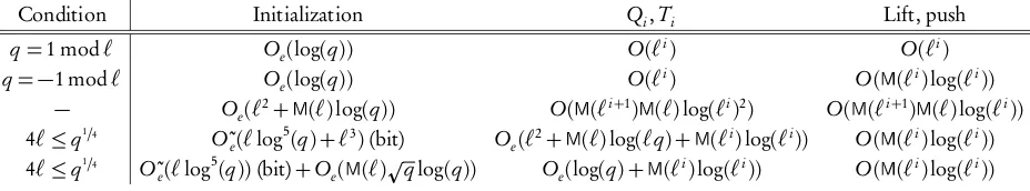
![Figure 3.1: The new square root algorithm vs. the one in [6]](https://thumb-us.123doks.com/thumbv2/123dok_us/7746357.1269285/38.612.178.433.378.558/figure-new-square-root-algorithm-vs.webp)