Gottfried Herold, Elena Kirshanova, and Alexander May
Horst G¨ortz Institute for IT-Security Faculty of Mathematics Ruhr University Bochum, Germany
Abstract. We provide for the first time an asymptotic comparison of all known algorithms for the search version of the Learning with Errors (LWE) problem. This includes an analysis of several lattice-based approaches as well as the com-binatorialBKWalgorithm. Our analysis of the lattice-based approaches defines a general framework, in which the algorithms of Babai, Lindner-Peikert and several pruning strategies appear as special cases. We show that within this framework,
alllattice algorithms achieve the same asymptotic complexity.
For theBKWalgorithm, we present a refined analysis for the case of only a poly-nomial number of samples via amplification, which allows for a fair comparison with lattice-based approaches. Somewhat surprisingly, such a small number of samples does not make the asymptotic complexity significantly inferior, but only affects the constant in the exponent.
As the main result we obtain that both, lattice-based techniques andBKWwith a polynomial number of samples, achieve running time 2O(n)forn-dimensional LWE, where we make the constant hidden in the big-Onotion explicit as a simple and easy to handle function of allLWE-parameters. In the lattice case this func-tion also depends on the time to compute aBKZlattice basis with block sizeΘ(n). Thus, from a theoretical perspective our analysis reveals howLWE’s complexity changes as a function of theLWE-parameters, and from a practical perspective our analysis is a useful tool to chooseLWE-parameters resistant to all known at-tacks.
Keywords.LWE security, Bounded Distance Decoding, Lattices,BKW
1
Introduction
Lattice-based cryptosystems are currently the best candidates for post-quantum security and allow for a variety of new functionalities. This led to an impressive amount of publications within the last decade (see e.g. [43],[19], [41] and their follow-up works). The security of most lattice-based public-key encryption schemes relies on the hardness of the Learning with Errors (LWE) problem – an average-case hard lattice problem introduced into cryptography by Regev ([43]), and formerly studied in the learning community ([21, 13]). In the search version ofLWE, one has to recover a secret vector s∈Znqby looking atmsamples(ai,hai,si+ei), whereai∈Znqis chosen uniformly at
random andei is a discrete Gaussian error with (scaled) standard deviations. Notice
that the input size of such anLWEsample is linear inn,logqand logs.
standard complexity assumptions ([20]), but the currently best algorithms for finding shortest vectors even with polynomial approximation ratio require either exponential time and space 2O(n)([3, 39]) or for polynomial space slightly super-exponential time 2O(nlogn)([26]).
While Regev’s quantum reduction fromSIVPtoLWEis dimension-preserving, Peik-ert’s classical reduction [40] has a quadratic loss by transformingn-dimensional lattice problems inton2-dimensionalLWEinstances inpolynomialtime (see also [14]) . These complexity theoretic results stress the need to studyLWE’s complexity directly in order to be able to instantiateLWEin cryptography with a concrete predetermined security level.
For the LPN problem, which is a special case of LWE for q=2, Blum, Kalai and Wasserman (BKW, [13]) designed the currently fastest algorithm with slightly sub-exponential complexity 2O(lognn)(see also the discussion in Regev [43]). Unfortunately, BKWrequires the same sub-exponential amount of memoryandofLPNsamples. Recent research [4, 5] analyzesBKW’s complexity in theLWE-setting forq=poly(n), where the authors provide fully exponential (inn) bounds for the runtime, as well as for memory and sample complexity.BKW’s huge sample complexity makes the algorithm often use-less forLWEcryptanalysis in practice, since cryptographic primitives like encryption usually provide no more than a polynomial number of samples to an attacker.
Concerning lattice-based attacks, the algorithm of Lindner and Peikert [32], which is an adaptation of Babai’sNearestPlanealgorithm to theLWEsetting, and its im-provements due to Liu-Nguyen ([33]) and Aono et al. ([8]) are considered as the practi-cal benchmark standard in cryptanalysis to assessLWE’s security. Unfortunately, the au-thors do not provide an asymptotic analysis of their algorithms as a function of theLWE
parameters(n,m,q,s). This is an unsatisfactory situation, since it makes lattice-based approaches somewhat incomparable among themselves and especially to the combina-torialBKW-algorithm in theLWEscenario [4, 7, 29]. The lattice-based literature often suggests that lattice-based approaches are most practical for attackingLWE, while the BKWliterature suggests that asymptotically theBKWalgorithm always outperforms lat-tice reduction. Our results show that both statements should be taken with care. It really depends on theLWE-parameters (and the lattice reduction algorithm) which approach is asymptotically fastest, even when we useBKWrestricted to only a linear numbermof samples.
WhetherLWE-type cryptosystems will eventually be used in practice crucially de-pends on a good understanding of the complexity ofLWE-instances. A proper cryptana-lytic treatment of a complexity assumption such asLWEincludes practical cryptanalysis of reasonably sized instances as well as an extrapolation to cryptographic security level instances fromasymptotic formulas. This is the widely accepted approach for estimat-ing key sizes [30, 1], which is for instance taken for measurestimat-ing the hardness of factorestimat-ing RSA-1024 [28]. Whereas some practical experiments on concreteLWEinstances where reported in the literature [32, 33, 8], the asymptotics remains unclear. Our work fills this gap.
com-plexity analysis of the LWEproblem that covers techniques such as lattice-based ap-proaches (lattice-basis reduction+enumeration, embedding) and the combinatorialBKW -approach. We state the algorithmic complexity regarding the three metrics: expected running time, memory complexity and number of LWEsamples, all as a function of theLWE-parameter(n,q,s). For attaining our results, we introduce the following tech-niques.
1. We propose a new generalized framework for Bounded Distance Decoding (BDD) enumeration techniques, which we callgeneralized pruning. Our framework cov-ers all previously known enumeration approaches such as Babai’sNearestPlane algorithm, itsLWE-extension NearestPlanes of Lindner-Peikert ([32]), Linear Pruning ([45]) and Extreme Pruning ([17]), which were left without rigorous anal-ysis in [6]. We show thatallthese approaches achievethe sameexpected running-timeϒ=2c f(n)havingthe sameconstantc. Of course, we should stress once again
that our analysis is purely asymptotic (as opposed to [6]). So in practice some prun-ing strategies clearly outperform others, as reported in several experiments in the literature [32, 33, 8], but our analysis shows that this superiority vanishes for in-creasingn.
To provide a complete picture of lattice-based attacks, in Sect. 5 we also include the asymptotic complexity analysis ofLWEusing Kannan’s embedding technique [26]. See Table 1 for the precise complexity estimates.
2. In Sect. 7 we refine the asymptotic complexity analysis of theBKWalgorithm in the case where onlym=O(nlogn)samples are given. This amplification of samples is similar to Lyubashevsky’s amplification for the LPN-case [34]. However, whereas theLPN-case amplification raised the running time from 2O(lognn) to 2O(log logn n), in the LWE case the loss affects only the constant. Again, see Table 1 for a more precise statement of the running time as a function of theLWE-parameters.
Since any lattice-based attack relies on a basis-reduction as preprocessing, its run-ning time crucially depends on the complexity of basis reduction. The basis reduc-tion algorithms of Kannan ([25]) or MV, ADRS, Laarhoven ([39, 2, 29]) have run time complexities 2Θ(nlogn) or 2Θ(n), respectively. We denote in Table 1 byc
BKZ the hidden
constant in these run time complexities. We write theLWEparametersq=ncq,s=ncs, where typicallycq,csare constants in cryptographic settings. For completeness, we also
include the performance of the Arora-Ge algorithm ([10]) in Table 1, an algebraic attack onLWEthat achieves sub-exponential running time forcs<12.
Notice that single exponential lattice reduction algorithms such as MV and ADRS ([39, 2]) lead to running time 2cnas in theBKW-case. Also from Table 1 one can already see that lattice-based attacks asymptotically outperformBKW(even with an exponential number of samples) as soon as the lattice reduction exponentcBKZis small enough, since
in all lattice attacks the denominator is quadratic incq−cs, whereas it is linear incq−cs
forBKW. Our results show quantitatively how the hunt for the best run time exponent for lattice reduction [39, 2, 29] directly affectsLWE’s security.
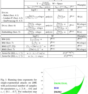
In Figure 1 we compare the behaviour of the constantcfor various algorithms and typical values. Here, the (heuristic) probabilistic sieving method of Laarhoven ([29]) with a runtime exponent ofcBKZ=0.33 already outperforms theBKWalgorithm for some
Table 1: Asymptotic comparison ofLWEdecoding algorithms. We denoteq=O(ncq), s=O(ncs)andc
BKZis the constant hidden in the run time exponent of lattice reduction.
For Arora-Ge, 2≤ω<3 is the linear algebra constant.
Complexity
ϒ=PT(ALG)
succ(ALG), M=Space #Samples TBKZ=2cBKZnlogn,MBKZ=poly(n) TBKZ=2cBKZn,MBKZ=2Θ(n)
log(ϒ) M log(ϒ) M
ENUM:
2cBKZ·cq
(√2cBKZ+cq−cs)2nlogn poly(n)
2cBKZ·cq
(cq−cs)2n 2
Θ(n) Θ(n)
– Babai (Sect. 4.1) – Lindner-P. (Sect. 4.2) –GenPruning(S. 4.3) DUAL(Sect. 6)
2cBKZ·cq
(cq−cs)2·nlogn poly(n)
2cBKZ·cq
(cq−cs)2·n 2Θ(n) Θ(nlogn)
2cBKZ·cq
(cq−cs+1/2)2·nlogn
2cBKZ·cq
(cq−cs+1/2)2·n 2
Θ(n)
Embedding (Sect. 5) 2cBKZcq
(cq−cs)2·nlogn poly(n)
2cBKZcq
(cq−cs)2·n 2
Θ(n)
Θ(n)
log(ϒ) M #Samples
BKW([4]) 12 cq
cq−cs+1/2·n 2
Θ(n)
2Θ(n) BKW(Sect. 7) 12 cq
cq−cs·n 2
Θ(n)
Θ(nlogn) BKW2([27, 22]) 1/
cq+2 ln(cq/cs)
−1
·n 2Θ(n) 2Θ(n)
BKW2(Sect. 7) 2 ln(cq/c s)
−1
·n 2Θ(n) Θ(nlogn)
Arora-Ge ([6]),cs<1/2 ω·(1−2cs)·n2cslog2(n) O(2n cslog2n
)
Arora-Ge ([6]),cs≥1/2 ω·(2cs−1)·nlog(n) O(2nlogn)
Fig. 1: Running time exponents for single-exponential attacks on LWE
withpolynomialnumber of samples for parameters cq∈[1.6. . .4.6] and
cs∈[0.1. . .0.7]. For reduction step
we havecBKZ=1 [2] (green plot) and
allowing heuristics as in [29]cBKZ=
2
Background
We use bold lower-case letters for vectors b and we let kbk denote their Euclidean norm. We compose vectors column-wise into matrices. For a linearly independent set B= (b1, . . . ,bk)∈Rn, thefundamental domainP1/2(B)is
∑ki=1cibi:ci∈[−12, 1 2) . The Gram-Schmidt orthogonalisation (basis) Be= (eb1, . . . ,ebk) is obtained iteratively by setting eb1=b1 andebi as the orthogonal projection of bi on (b1, . . . ,bi−1)⊥ for i=2, . . . ,k. In this work we deal with so-calledq-ary latticesΛ (i.e.qZn⊆Λ ⊆Zn)
generated by a basisB= (b1, . . . ,bn)∈Znq:
Λ =L(B) =
n n
∑
i=1
zi·bi modq:zi∈Z
o
.
There are several hard problems that we can instantiate on lattices. The closest vector problem (CVP) asks to find a lattice point v closest to a given point t∈Rn. In the
promise variant of this problem, known as Bounded Distance Decoding (BDD), we have some boundRon the distance between the lattice andt:kv−tk ≤R, whereRis usually much smaller than the lattice’s packing radius.
For two discrete random variablesXandY with rangeS, thestatistical distance be-tweenXandY is SD(X;Y) =12∑s∈S|Pr[X=s]−Pr[Y=s]|. The min-entropy function
is denotedH∞(X) =−log maxs∈S{Pr[X=s]}.
Discrete Gaussian Distribution. To each lattice-vectorv∈Λ we can assign a proba-bility proportional to exp(−πkvk2/s2)for the Gaussian parameter1s>0 (see e.g. [19] for a sampling algorithm). We call the resulting distribution havingΛ as support the discrete Gaussiandistribution.
For integer lattices, a sufficiently wide discrete Gaussian blurs the discrete struc-ture ofΛ(more formally,s=poly(n)exceeds the smoothing parameter [37] ofZnfor
cs> 12), such that the distribution becomes very close to a continuous Gaussian ([41],
[32]). In our analysis, we make use of continuous Gaussians to estimate the success probability of our decoding algorithms.
We use the following well-known tail bound for Gaussians. For fixedsandy→∞:
1−
Ry −yexp(−πx
2 s2 )dx
s =e
−Θ(y 2
s2) 1−
∑yx=−yexp(−πx 2 s2 )
∑∞x=−∞exp(−π
x2 s2 )
=e−Θ( y2
s2) . (1)
Learning with Errors. TheLearning with Errorsproblem ([43]) is parametrized by a dimensionn≥1, an integer modulusq=poly(n)and an error distributionDonZ.
Typically, Dis a discrete Gaussian on with parameters. For secret s∈Zn
q, an LWE
sample is obtained by choosing a vectora∈Zn
quniformly at random, an errore←D,
and outputting the pair(a,t=ha,si+emodq)∈Zn
q×Zq. Having a certain numberm
of such pairs, we can write this problem in matrix form as(A,t=Ats+emodq)for
t= (t1, . . . ,tm),e= (e1, . . . ,em)and the columns of matrixA∈Znq×mare composed of
theai. Overall, theLWEproblem is given by parameters(n,q,s)andm(this parameter
we can choose ourselves). Typically, (n,q,s) are related as q=O(ncq),s=O(ncs),
1Fors→
and 0<cs <cq are constants. If not specified otherwise, we assume these relations
throughout.
Thesearchversion of theLWEproblem asks to finds, thedecisionversion asks to distinguishtfrom a uniform vector, givenA. TheLWEproblem is an average-case hard Bounded Distance Decoding problem for theq-ary latticeΛ(At) ={z∈Zm:∃s∈Znq
s.t.z=Atsmodq}. AssumingAis full-rank, its determinant is det(Λ(At)) =qm−n. Lattice basis reduction.The goal oflattice basis reductionalgorithms is to make some input basis as short and orthogonal as possible. The algorithm that is most relevant in practice is a block-wise generalization of theLLL-algorithm, calledBKZalgorithm. There are two approaches to express the complexity of theBKZalgorithm. The first approach is via the so-calledHermite factordefined asδm=kb1k/vol(L)
1
m, for an m-dimensional latticeL, whereb1is the shortest vector of the output basis. The Hermite factor, introduced in [18], indicates how orthogonal the output basis is (we haveδ ≥1,
with equality for an orthogonal basis).
The second approach – rather than relying on the output parameterδ – relates the
running time of theBKZto the input block-sizeβ. As a subroutine,BKZcalls anSVP -solver in a sub-lattice of dimensionβ. In [23], the authors show that after a polynomial
(in m) number of SVP-calls, BKZwill produce a basis where the first (i.e. shortest) vector satisfies
kb1k ≤2(β)
m
2β·(detL) 1
m. (2)
Thus, the running time ofBKZisTBKZ=poly(m)·TSVP(β), whereTSVP(β)is the running time of an SVP-solver in dimensionβ. With current algorithms, it is at least exponential
inβ, and has been improved from 2O(β2) ([16]), to 2O(βlogβ) in [25], and recently to
2O(β) in [39] (the latter has also 2O(β) memory complexity). There is no analogous result proven for the complexity ofBKZin terms ofδ.
Geometric Series Assumption(GSA), proposed by Schnorr ([44]), provides an esti-mate on the length of the Gram-Schmidt vectors of aBKZ-reduced basisB. It assumes that the sequence ofkebik’s decays geometrically ini, namely,
kebik
kebi+1k
≈δ2. Thus, GSA
allows us to predict the lengths of all Gram-Schmidt vectors askebik ≈ kb1k ·δ2(1−i). From the analysis of [23], it follows that in terms ofβ, GSA can be stated as
kebik ≈ kb1k ·β−
i
β. (3)
In our asymptotic analysis we treat the above Eq. (3) as an equality2, which is the worst-case for the length of the shortest vector returned by BKZreduction: we have kb1k=β
m
2β·(detL)m1. Equivalently, for anLWElatticeΛ(At),kb1k=β
m
2β·q1−mn. This follows from the fact that the product of all Gram-Schmidt vectors is equal to the lattice-determinant.
We note here that according to [23], the above relation should only hold for the first m−β Gram-Schmidt vectors. Indeed, a worst-case analysis [24] shows that the last
Gram-Schmidt vectors behave likekebik ≈exp(−41log(d−i)2), showing a faster decay
than GSA suggests. In this paper, however, we stick to Eq. (3), as it greatly simplifies the exposition. Note that we can ameliorate the effect of this discrepancy on our analysis
byBKZ-reducing the dual of the lattice and taking the dual of the returned basis, so the faster decay occurs during the first (rather than the last) Gram-Schmidt vectors.
3
LWE Decoding
This section gives an extended roadmap to the subsequent sections: we briefly describe the existing methods to solve thesearchLWEproblem, for each of which we present a complexity analysis. For all the approaches considered, we are interested in the quantity
ϒ(ALG) = PT(ALG)
succ(ALG), the time/success trade-off. The decoding of an LWE instance
(A,t=Ats+emodq)is successful, when the returned error-vector is indeed e(or, equivalently, we return the lattice-vectorAts).
Currently, there are three conceptually different ways to approach LWE: lattice-based methods, combinatorial methods and algebraic methods. The lattice-lattice-based meth-ods, in turn, can also be divided into three approaches: we can first viewLWEas aBDD
instance for the latticeΛ(At), or second we apply Kannan’s homogenization technique to convert theBDDinstance into a unique-SVPinstance by adding the target vectortto a basis ofΛ(At)and search for the shortest vector in a lattice of increased dimension, or third, we can target the decisionLWEproblem by solving approximate-SVPin the dual lattice. In this work, we primarily focus onBDD, while presenting only shortly the complexity of unique-SVPembedding forLWEin Sect. 5 and the dual approach in Sect. 6.
As for combinatorialBKW-type methods ([13], [4]), to recoverswe apply a Gaussian elimination approach in the presence of errors, where we allow to multiply our equa-tions only by±1 to keep the error small. In other words, we queryLWEsamples(a,t)
until we find pairs that match (up to sign) on some fixed coordinates, add them up to obtain zeros on these coordinates and proceed on the remaining non-zero parts. Once a sample with only one non-zero coordinate(a00s0+e00,t0)is obtained, we brute-force ons0(the errore00, being the sum of all the errors used to generate this sample, is very large compared to the initialei’s and we cannot conclude ons0immediately). Recent improvements ([27, 22]) only require small coordinates (rather than zero). As opposed to the lattice-based attacks, theseBKW-type methods succeed with high probability on a random matrixA, provided we can query for exponentially many samples. This con-dition, however, is unrealistic: the number ofLWEsamples exposed by a primitive is typically only poly(n), possibly onlyO(n). Thus, in Sect. 7, we are mainly concerned with the analysis of the so-calledamplificationtechnique, where out ofΘ(nlogn)(or evenΘ(n))LWEsamples, one is able to construct ‘fresh’ samplessuitableforBKW.
As for lattice-based methods,BDDdecoding is a two-phase algorithm: first, a ba-sis for Λ(At)is preprocessed viaBKZ-reduction to obtain a guarantee on the quality of the output basis (the length of the Gram-Schmidt vectors). With this, we form a search space for the second phase, where we enumerate candidates for the error-vector ewithin this search space. Among various ways to enumerate, we start with the greedy approach: Babai’sNearestPlanealgorithm ([11]), then consider its extension, Linder-PeikertNearestPlanes ([32]), and finally, pruning strategies ([17], [33]) applied to
ϒ(ENUM) =PT(ENUM)
succ(ENUM) for the second phase takes the same value in the leading-order term, including the constant in front. Of course, the ‘real’ trade-off of the wholeLWE
attack isϒ(BDD) =T(BKZP)+T(ENUM)
succ(BDD) , but as we show below, the second phase – enu-meration – dominates over the reduction phase. Now we give a high-level idea of the mentioned enumeration algorithms, where we focus on their geometric meaning. A
BDDinstance(B={b1, . . . ,bm},t∈L(B) +e)with a promise onkekis received as
input.
Babai’s NearestPlane.A recursive description of this algorithm is convenient for our later analysis. Given a targett∈Zmand anm-dimensional lattice3L(b1, . . . ,bm),
we search for cm∈Z such that the hyperplaneUm=cmebm+Span(b1, . . . ,bm−1) is the closest tot. In other words,Umis the span of the closest translate of the(m−1)
-dimensional lattice L(b1, . . . ,bm−1). We save this translate (storingcm), sett0as the
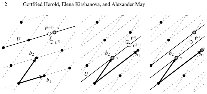
projection ofton Span(b1, . . . ,bm−1)and call the algorithm recursively with new lower-dimensional targett0andL(b1, . . . ,bm−1). Aftermrecursive calls, we trace back the translatesci’s and the lattice-vector∑mi=1cibiis returned. In Figure 2a, a 2-dimensional
example is shown: the hyperplaneU spans the closest translate ofL(b1)tot(m). The algorithm is clearly polynomial-time inm, but how can we guarantee that the returned lattice-vector is indeed the closest?
It is easy to verify that the algorithm succeeds if the error vector of theBDDinstance lies inP1/2(eB), the fundamental parallelepiped of the Gram-Schmidt basisBe. Indeed, the distance to the closest translate on each call is bounded by 12kebik. Thus, we stay
insideP1/2(Be)during the execution. How likely is it that the originaleis inP1/2(Be)? This depends on the quality of the input basisB, i.e. the length of the Gram-Schmidt vectors. As we have a guarantee onkekand the quality ofB, in Sect. 4.1 we estimate the success probability of Babai’s algorithm, and hence, the ratio PT(BABAI)
succ(BABAI).
Lindner-PeikertNearestPlanes.The success probability of Babai’s algorithm is low, in fact, super-exponentially low for small choices of block sizeβ. Roughly, the length of
the error-vector output by Babai’s algorithm can be as large as∑mi=1kebik2, and so might
be even larger thanb1, which contradicts theBDDpromise. An extension of Babai’s al-gorithm was proposed in [32], where the authors suggest to consider not only the closest translate, but rather several close ones on each recursive call. Thus, we have several can-didate solutions in the end. The approach takes into account the skewness of the input basis: taking a further hyperplane in one call might result in much closer hyperplanes on subsequent calls, thereby decreasing the overall error-length. This is illustrated in Figure 2c, where the 3 closest translates ofL(b1)are chosen and the solution lies on a further translate. The number of hyperplanesUi=ciebi+Span(b1, . . . ,bi−1)we choose on levelidepends on the length ofebi: the shorter this vector is, the more skewed the
lattices in this dimension is, the more hyperplanes we should choose to offset the error. Following [32], bydiwe denote the number of differentci’s onith level. The resulting
search-space is then a stretched fundamental parallelepipedP1/2(eB·D), whereDis the diagonal matrix of alldi’s. Babai’s algorithm is the special case withD=I.
What can we say now about the running-time/success probability? For the latter, we surely can guarantee a constant success probability by making thedi’s sufficiently large.
In Sect. 4.2, we estimate the running time for the case of constant success probability. Length-pruning and variations.The choices of hyperplane(s) inNearestPlane(s) do notdepend on the error-length we have accumulated so far: we hope that our cur-rentlychosen projection (target) will have relatively close hyperplanes in the subsequent recursive calls contributing to the error-length as little as possible. In other words, ex-pressing the output error-vector via the Gram-Schmidt basis,e0=∑mi=1e
0 i
e
bi
kebik
, we bound the coordinates|e0i|individually.
Algorithms that put constraints on the so far accumulatedtotal error-lengthwhile choosing a hyperplane, so-called length-pruning strategies, were proposed forSVPin [45], extensively studied in [17] and adapted to BDD in [33]. The boundRi that we
impose on the accumulated total length at theith level is specific to the length-pruning strategy under consideration.
For instance, taking into account the Gaussian nature ofLWE-error, one can use tail-bounds for Gaussians and estimate the final error length asR=Θ(s√m). So we could useRi=Ras a trivial bound, having a spherical search space, which guarantees constant
success probability. We refer to this asspherical pruning. More interesting is setting Ri= (m−mi+1)
1
2·Ras bounds on the error-length on theith level (countingidownwards). This case is calledlinear pruning([45]). Furthermore, instead of having a linear decay, one can think of other bounding functions. [17] considers various choices forRi and
analyzes the running-time/success probability ratioϒ(ENUM)of these algorithms by
comparingϒ(ENUM)with the corresponding ratio of spherical pruning.
In Chapter 4.3, we take a more general approach: we consider generalized pruning algorithms that put bounds on the current|e0
i|, where the bound arbitrarily depends on
the already accumulatedej’s for j>i. This covers Babai’s, the Lindner-Peikert
algo-rithm, as well as length-pruning strategies. We then give conditions that a reasonable pruning strategy should meet and analyze the trade-offϒ=PT(ENUM)
succ(ENUM). We show thatϒ is asymptotically the same foranyreasonable generalized pruning strategy.
4
LWE Decoding: General Strategies
In this section, we consider algorithms for solving theLWEproblem via bounded dis-tance decoding. In this approach, we first compute a reduced basis forΛ(At)(the
4.1 Babai’sNearestPlane(s)algorithm
Suppose we are a given a shift4x∈
Qmand a basisB=B(m)={b1, . . . ,bm} ∈Zmfor
the shifted latticex+L(B(m))as well as a target pointt=x+v+e∈x+SpanL(B). In the context ofLWEdecoding, the shift isx=0 in the inital call and we know thateis small. Our task is to recoverx+vor, equivalently, the error vectore. Babai’s algorithm for this works as follows: we can writex+L(B(m))as
x+L(B(m)) =[ i∈Z
x+ibm+L(b1, . . . ,bm−1).
x+ibm+L(b1, . . . ,bm−1)⊂Uiis contained in them−1-dimensional hyperplane
Ui:=
n y∈Rm
D
y, ebm
kebmk2 E
=i+Dx, ebm
kebmk2 Eo
. (cf. Fig. 2a)
Babai’s algorithm orthogonally projectst=t(m)onto theUithat is closest tot(m)to
ob-taint(m−1)and then recursively solves the problem fort(m−1)and the shifted sublattice
(x+ibm) +L(b1, . . . ,bm−1). Formally, we obtain the following algorithm:
Algorithm 1Babai’sNearestPlane(B,x,t,e0)
Input: B= (b1, . . . ,bk)∈Zm×k,x∈Qm,t∈x+SpanB,e0∈Qm (e0=x=0 in inital call)
Output: v∈x+L(B)close totande0=t−vcorresponding error vector
1: x(k)←x,t(k)←t,e0(k)←e0. LeteB←GSO(B). .For notational purposes
2: ifk=0then return(x,e0)
3: Computeu(oldk)←
t(k), ebk
kebkk2
4: Chooseu(newk)=
x(k), ebk
kebkk2
+i(k)closest touold(k)withi(k)∈Z. 5: x(k−1)←x(k)+i(k)b
k .x(k−1)+L(B(k−1))is nearest plane 6: e0(k−1)←e0(k)+ (u(oldk)−u
(k)
new)bek,t(k−1)=t(k)−(u
(k)
old−u
(k)
new)ebk .Project onto this plane 7: returnNearestPlanes((b1, . . . ,bk−1),x(k−1),t(k−1),e0(k−1))
For notational consistency with later algorithms, the argumente0keeps track of the error vector accumulated so far and is 0 in the initial call. Note that the algorithm constructs the error vectore0coordinate-wise (wrt. the Gram-Schmidt basisBe), starting fromebm.
Analysis.Babai’sNearestPlanesalgorithm runs in polynomial time. In the context of LWE decoding, we want that e0 output by the algorithm equals the LWEnoise e. Writee=∑kekkebk
e
bkk
in the Gram-Schmidt basis. We havee=e0if all the algorithm’s choices of nearest planes are the correct ones, which happens whenever|ek|<12kebkk for all k, i.e. if eis in the interior of P1/2(Be). The algorithm fails if|ek|>12kebkkfor anyk.5For the analysis, we approximate the discrete Gaussian noiseeby acontinuous one, so the ek are independent Gaussians with parameter s. For our parameters, the
4This is equivalent to the problem for target vectort−xand without shift. We use shifts to write the algorithms in a cleaner way via recursion, where shifts will appear in the recursive calls. 5On the boundary ofP
1/2(eB), it depends on how equally close hyperplanes are handled in line 4
case of interest iskebmk s keb1k: in the first steps of the algorithm, we haves kebmk,kebm−1k, . . ., which contributes to a superexponentially small success probability. Thekebkkincrease geometrically (under GSA) fromkebmktokeb1k. At some intermediate criticalk∗, we haves≈ kebk∗kand the subsequent steps do not contribute much to the
failure probability. More precisely:
Lemma 1. Let the sequencekeb1k> . . . >kebnkbe geometrically decreasing with decay
ratekebik/kebi+1k=δ2>1. Let e1, . . . ,enbe independent continuous Gaussians with
density 1sexp(−πx2
s2 ). Let pi:=Pr
|ei|<kebik. Then
– Ifkebnk>s(logn)
1
2+εfor fixedε=Θ(1),ε>0, then∏ipi=1−o(1). – Ifkebnk=s, then∏ipi=2−O(n).
– Ifkeb1k=s, then∏ipi=2−O(n)·2nδ−n(n−1).
Proof. By Eq. (1), 1−pi is superpolynomially small ifkebik>s(logn)
1
2+ε. The first statement then follows by a union bound. The second statement is trivial, as we have minipi=Ω(1). For the third statement, we estimate forkebik<s
pi=
Z +kebik
−kebik 1 se
−πx2
s2dx=Θ(1)
Z +kebik
−kebik 1
sdx=Θ(1) kebik
s/2.
So∏ipi=2−O(n)∏ kebik
(s/2)n =2−O(n)
2n keb1kkebnk n/2
sn =2−O(n) 2nk
e
bnkn/2 sn/2 =2
−O(n)2n
δ−n(n−1).
This implies the following theorem for Babai’sNearestPlanesalgorithm:
Theorem 2. Under the Geometric Series Assumption (GSA) on aβ=Θ(n)
reduced-basis that arises from m= (cm+o(1))nLWEsamples with parameters(n,q=O(ncq),
s=O(ncs))for c
m and cs<cqconstants, Babai’sNearestPlanesalgorithm solves
the search-LWEproblem in polynomial time with success probability
Psucc(BABAI) =
2−12 2mβ−cq+c
−1 m cq+cs
2
(1+o(1))βlogβ
, if 2βm −cq+cm−1cq+cs>0
1−o(1), if 2βm −cq+c−m1cq+cs<0,
if we assume that theLWEerror follows a continuous Gaussian distribution.
Note that the two cases in the theorem relate to whetherkb1kis larger or smaller thans.
Proof. Under GSA, we havekebik=β
m
2βq1−cm−1δ−2iwithδ =β 1
2β. A simple computa-tion shows thatkebk∗k=ncs for the criticalk∗=β(m
2β+cq−cqc
−1
m −cs). Consequently,
m−k∗=β 2βm −cq+mncq+cs. (4)
If2βm −cq+c−m1cq+cs>0, we actually havek∗>mandkebmk>s·poly(n). The success
probability is 1−o(1)by the first part of Lemma 1. If 2βm −cq+c−m1cq+cs<0, by the
third part of that lemma, we have
Psucc(BABAI) =2
−O(m)2m−k∗
δ(m−k
∗)2
=2− 1
2 2mβ−cq+
n
mcq+cs+o(1) 2
βlogβ
b2
b1
t(k) U
t(k−1) v
(a)Babai’sNearestPlaneAlgorithm for a good basis. A target pointt(k)is projected on
a closest hyperplane 2b2+Span(b1).The re-cursive call for the chosen one-dimensional subspaceU(thicker) projects on the closest zero-dimensional hyperplane - the shaded lat-tice pointv.
b2 b1
t(k)
U
t(k−1)
v
(b) Babai’s NearestPlane Algo-rithm for a bad basis. Now the closest hyperplane isb2+Span(b1). The cho-sen one-dimensional subspaceUhas changed, so has the vector v. Obvi-ously, this lattice vector is not the so-lution.
b2 b1
t(k)
v
(c) In Lindner-Peikert’s general-ization, we stretch the bad ba-sis case by settingd2=3 in di-rections 2b2,b2,0b2,and recurse on each. The process collects all shaded points and therefore also the closest one.
Fig. 2:NearestPlane(s)Algorithms
4.2 Lindner-PeikertNearestPlanesAlgorithm
Babai’s algorithm is characterized by itssearch region VBabai=P1/2(eB). Indeed, it returns the unique6v∈L(B)witht∈v+P1/2(Be). Therefore, the more orthogonal the input basis Bis, the better v approximates the lattice-vector closest tot(in Figure 2a the basis vectors are fairly orthogonal). However, the procedure performs far worse if a given basis is ‘long and skinny’ (Figure 2b) and the error increases as the dimension grows. In terms of theLWEdecoding problem this means that Babai’sNearestPlane will solve the search LWE-problem iff the error vector elies in P1/2(Be). For typical parameters, this is rather unlikely since the last Gram-Schmidt vectors in aBKZreduced basis are fairly short.
To address this problem, Lindner and Peikert suggested to choose several (di≥1)
close hyperplanes in theith level of the recursion (Figure 2c). Geometrically, this means that we stretch the elongated parallelepipedP1/2(Be)to a cube-like shape by increasing the last and therefore short Gram-Schmidt vectors. In the end, we havedm· · ·d1 candi-date solutions to check. Formally, the algorithm works as follows:
Algorithm 2Lindner-Peikert’sNearestPlanes(B,x,t,e0)
Input: B= (b1, . . . ,bk)∈Zm×k,x∈Qm,t∈x+SpanB,e0∈Qm (e0=x=0 in inital call)
Output:A set of pairs(v,e0)withv∈x+L(B)ande0=t−vcorresponding error vector 1: x(k)←x,t(k)←t,e0(k)←e0. LeteB←GSO(B). .For notational purposes
2: ifk=0then return{(x,e0)}
3: Computeu(oldk)←
t(k), ebk
kebkk2
4: Letu(jk)=
x(k), ebk
kebkk2
+i(jk)fori(jk)∈Z,j=1, . . . ,dkbe thedkclosest numbers tou
(k)
old. 5: Letx(jk−1)←x(k)+i(k)
j bkfor 1≤j≤dk .x
(k−1)
j +L(B
(k−1))are thed
knearest planes 6: e0j(k−1)←e0(k)+ (u(k)
old −u
(k)
j )bek,t
(k−1)
j =t
(k)−(u(k)
old−u
(k)
j )ebk, .Project onto them 7: returnS
jNearestPlanes((b1, . . . ,bk−1),x
(k−1)
j ,t
(k−1)
j ,e
0(k−1)
j )
Analysis.Our search region is now extended toVLP=P1/2(eB·D), which, as estimated in [32], amplifies the success probability forLWEdecoding to
PLP:=Pr[e∈P1/2(Be·D)] =
m
∏
i=1 Prh
e,ebi<di
·kebik2 2
i
= m
∏
i=1
erfdikebik
√
π 2s
,
whereDis the diagonal matrix composed of thedi’s, and erf(x) = √2πR0xe−t 2
dt. Here, like in Sect. 4.2, we estimate the discrete Gaussian erroreby a continuous one. We wish to set the parametersdisuch that the success probability is at least constant. It follows
from Eq. (1) that if min1≤i≤mdi kbik
s =ω(
√
logm), thenPLP=1−o(1). Conversely, if we have min1≤i≤mdi
kbik
s =o(1), thenPLP=o(1). So we setdi=
s·(logm)α
kebik
for sufficiently largeα>1/2 (which will not affect the asymptotic running time anyway). Note that for our parameter choices,keb1kwill be much larger thans, so the firstdi’s in the algorithm
are all equal to 1 and the sequence of thedi’s has the form(1,1, . . . ,1,2, . . .).
Let us turn our attention to the running time. The recursive calls to the Linder-Peikert algorithm have the structure of a rooted tree, where the root corresponds to the initial call and every node calls itsdkchildren. The leaves correspond to the candidate
solutions we need to check in the end. Note that every node at levelk(the root has level mand the leaves have level 0) corresponds to a partial solution, where we already fixed the lastm−kcoefficients ofe0 (wrt. theBe-basis) and ofx(wrt. theB-basis). LetNk
be the number of nodes at levelkandN be the total number of nodes. Clearly,Nk= ∏mi=k+1diandN=∑mk=0Nk. As the running time per node is polynomial, estimating the
running time amounts to estimatingN. For this, we have the following result.
Theorem 3. Under the Geometric Series Assumption (GSA) on a β =Θ(n)-reduced basis that arises from m= (cm+o(1))nLWEsamples with parameters(n,q=O(ncq),
s=O(ncs))for c
mand cs<cqconstants,NearestPlaneswith our choice of di’s solves
search-LWEproblem with success probability1−o(1)in time
TLP=poly(n)N=
212 2mβ−cq+c
−1 m cq+cs
2
(1+o(1))βlogβ
, if 2βm −cq+cm−1cq+cs>0
and polynomial memory (using depth-first search), if we assume that theLWE error follows a continuous Gaussian distribution.
Proof. If m
2β−cq+c
−1
m cq+cs<0, we havekebmk>s·poly(m), so for sufficiently large
m, alldi=1 and the result follows from Thm. 2. So consider the case2βm −cq+c−m1cq+
cs>0. SinceNk≤N0for allk, we haveN0≤N≤(m+1)·N0. So up to polynomial factors, the running time is given by N0=∏di. Let the criticalk∗ be maximal, s.t.
kebk∗k>s. By Eq. (4),m−k ∗
β =
m
2β −cq+
n
mcq+cs. We compute forN0=∏idi:
m
∏
i=k∗+1 s
kebik
≤
m
∏
i=1 l
s·(logm)α
kebik m
=
∏
i
di=N0 and
N0≤(1+ (logm)α)m m
∏
i=1 l s
kebik
m
≤(1+ (logm)α)m2m−k∗ m
∏
i=k∗+1 s
kebik .
We already computed (the inverse of)∏mi=k∗+1kebs ik
in the analysis of Babai’s algorithm (cf. Lemma 1 and Thm. 2), so
m
∏
i=k∗+1 s
kebik =2
(m−k∗)2
2β2 +o(1)
βlogβ
,
which is exactly what we want. The error term(1+ (logm)α)m2m−k∗ =2O(mlog logm) only contributes to theo(1)-term.
4.3 Generalized Pruning Strategies
In Babai’s or Lindner and Peikert’s algorithm, at every node at levelkin the search tree, we have already fixed the coordinatese0m, . . . ,e0k+1of the output error vectore0=
∑ie0i
e
bi
kebik
(in the Gram-Schmidt basis). These coordinates are contained in the argument e0(k)=∑mi=k+1e
0 i
e
bi
kebik
Algorithm 3 Generalized Pruning AlgorithmGenPruning(B,x,t,e0)for a family of bounding functionsB(k)
Input: B= (b1, . . . ,bk)∈Zm×k,x∈Qm,t∈x+SpanB,e0∈Qm (e0=x=0 in inital call) Output:A set of pairs(v,e0)withv∈x+L(B)ande0=t−vcorresponding error vector
1: x(k)←x,t(k)←t,e0(k)←e0. LeteB←GSO(B). .For notational purposes
2: ifk=0then return{(x,e0)}
3: Computeu(oldk)←
t(k), ebk
kebkk2
. 4: Lete0i=he0(k), bi
kbikifork<i≤m. .Coefficients ofe
0
5: LetD2max=B(k)(em02, . . . ,e0k2+1) .bound on distance of next hyperplanes 6: Letu(jk)=
x(k), ebk
kebkk2
+i(jk), j=1, . . .be all possible numbers s.t.
|u(oldk)−u
(k)
j |2· kebkk2≤D2maxandi
(k)
j ∈Z. 7: Letx(jk−1)←x(k)+
i(jk)bkfor all j .Consider the nearby planesx
(k−1)
j +L(B
(k−1))
8: e0j(k−1)←e0(k)+ (u(k)
old −u
(k)
j )bek,t
(k−1)
j =t(k)−(u
(k)
old−u
(k)
j )ebk, .Project onto them
9: returnS
jGenPruning((b1, . . . ,bk−1),x
(k−1)
j ,t
(k−1)
j ,e
0(k−1)
j )
The algorithm recurses on all hyperplanes, s.t.(e0k)2≤B(k)(e02
m, . . . ,e0k2+1). So the search region ofGenPruningis given by
VGP=ne0=
∑
ie0i ebi
kebik e
02
k ≤B(k)(em02, . . . ,e0k2+1)for allk o
and the algorithm is successful if theLWEerror vector is contained inVGP.GenPruning captures what is known as pruned enumeration [45]: in pruned enumeration, we keep only partial candidate solutions where the partial error vectorse0(k)satisfyke0(k)k ≤Rk
for some level-dependent boundsRkthat are defined by the particular pruning strategy.
This is achieved by setting
B(k)(e0m2, . . . ,ek02+1) =R2k−
∑
i
e0i2. (5)
For instance, we get the following algorithms for those specific choices ofB(k):
– B(k)(e0m2, . . . ,e0k2+1) = kebkk 2
2
: Babai’s algorithm7. – B(k)(e0m2, . . . ,ek02+1) = dkkebkk
2 2
: Linder-Peikert algorithm. – B(k)(e02
m, . . . ,e0k2+1) =Θ(ms2)−∑mi=k+1e0i2: Spherical Pruning.
– B(k)(e02
m, . . . ,e0k2+1) =Θ((m−k−1)s2)−∑mi=k+1e0i2: Linear Pruning.
We also cover the extreme pruning approach of [17] and potential algorithms where B(k)has a more complicated dependency on the individuale0i’s. For technical reasons, we require thatB(k) is extended to real-valued arguments in a continuous way, so the algorithm becomes meaningful for error vectors following a continuous Gaussian and we analyze it for such continuous errors. Furthermore, the bounding functions do not get the Gram-Schmidt vectors or their lengthskebik as explicit inputs, but we rather
treat these lengths as a promise. Essentially, this mean that we restrict to enumeration algorithms that are oblivious to the actual geometry of the lattice.
Analysis.We are interested in the ratio of expected running time to success probability
ϒ(GP) = T(GP)
Psucc(GP)if theLWEerror vectorefollows a continuous Gaussian with parameter s. LetVkbe the search region at levelk, i.e.
Vk=
n e0=
m
∑
i=k+1 e0i ebi
kebik e
02
j ≤B(j)(e 02
m, . . . ,e 02
j+1),k<j≤m o
andNk be the number of nodes at levelkduring a run ofGenPruning. LetPk be the
probability that we retain the correct solution at levelk(i.e. we have a partial solution at levelkthat can be extended to the solution of the search-LWEproblem). Note thatNk
is the number of points ine−Vkthat belong to the latticeπk(L(B)), whereπkis the
projection onto the orthogonal complement of Span(b1, . . . ,bk). So, we expect that
Nk≈
volVk kebmk · · · kebk+1k
(6)
by what is known as the Gaussian Heuristic. Interestingly enough, we only require Eq. (6) to hold up to a factor 2O(m), which we can prove rigorously forconvex Vkand
taking the expected value (overe) ofNk, using a variant [42] of Minkowski’s Convex
Body Theorem. We will prove matching lower and upper bounds forϒ(GP), where for the upper bound we need to impose some (weak) restrictions on the bounding functions. Definition 4. Assume that thekebik follow the GSA and that our correct error vector
follows a continuous Gaussian with parameter s. Assume thatkeb1k>s>kebmkand
let k∗be maximal s.t.kebk∗k>s. We call B(k)resp. the associated generalized pruning
algorithmreasonablefor the given parameters if the following conditions are satisfied: 1. B(k)(em02, . . . ,e0k2+1) +∑im=k+1ei02=O(ms2).
2. Psucc(GP)≥2 −O(m)P
k∗.
3. Nk≤2O(m)Nk∗for k≤k∗.
4. Nk−1
Nk =Ω(1)for k≥k
∗.
5. Vk∗ is convex.
Condition 1 means that we do not consider partial solution where the accumulated error vector up to that level point is already larger than the expected the final error vector. Conditions 2 and 3 tell us that, up to exponential factors, we can find the correct so-lution at little cost, provided it survived until levelk∗. Note that switching to Babai’s algorithm from levelk∗on will ensure that conditions 2 and 3 hold. Condition 4 tells us that the average number of children nodes at leveliis at least constant as long as kebik<s. Note thatkebik<simplies that we always haveΩ(1)plausible candidate
hy-perplanes at distance at mosts. The convexity property holds for all pruned enumeration strategies that use Eq. (5) and may be replaced by asking that heuristic Eq. (6) holds up to exponential error.
Theorem 5. Under the Geometric Series Assumption (GSA) on a β =Θ(n)-reduced
basis that arises from m= (cm+o(1))nLWEsamples with parameters(n,q=O(ncq),
s=O(ncs)) for c
m and cs <cq constants, such that 2βm −cq+c−m1cq+cs>0, any
reasonable generalized pruning algorithmGPhas an expected running time to success probability ratioϒ of
ϒ(GP) =E[T(GP)]
Psucc(GP) =2
1
2 2mβ−cq+c
−1 m cq+cs
2
(1+o(1))βlogβ
.
Furthermore, if Eq.(6)holds up to at most an exponential factor then, even ifGPis not reasonable, the above is also alower boundforϒ(GP).
Proof. The running time is clearly poly(m)·∑iNi. If the pruning strategy is reasonable,
we have
Psucc(GP) =2O (−m)P
k∗ and T(GP) =poly(m)
∑
i
Ni=2O(m)Nk∗,
because Ni≤2O(m)Nk∗ for all i, no matter whether i>k∗ ori<k∗. Now, Nk∗ is the
number of points from e−Vk∗ in the lattice πk∗(L(B)). Hence, the expected value
(over the choice ofe) ofNk∗ is given by
E e[Nk
∗] =
∑
x∈πk∗(L(B))f(x) where f(x) =
Z
Vk∗ 1 sk∗exp(−
πkyk2
s2 )dy.
SinceVk∗ is convex, its characteristic function is log-concave. The Gaussian density is
log-concave. So f is the convolution of two log-concave functions, hence log-concave itself. In particular, f is centrally symmetric and quasiconcave. It follows by a variant of Minkowsi’s Convex Body Theorem due to R. Rado [42] that
E e[Nk
∗] = 2 ±O(m) det(πk∗(L(B)))
Z
f(x)dx= 2
±O(m)volV k∗
det(πk∗(L(B)))
. (7)
By Condition 1 in Def. 4, we have 1≥exp(−πx2 s2 )≥e
−O(m)for everyx∈V k∗. So
E[T]
Psucc(GP)
=
2±O(m) volVk∗
kebmk···kebk+1k
R
x∈Vk∗
1
sm−k∗exp(− πkxk2
s2 )dx
= 2
±O(m)sm−k∗
kebmk · · · kebk+1k
R
x∈Vk∗1dx
R
x∈Vk∗exp(−
πkxk2
s2 )dx
= 2
±O(m)sm−k∗
kebmk · · · kebk+1k
R
x∈Vk∗1dx
R
x∈Vk∗1dx
=212 2mβ−cq+c
−1 m cq+cs
2
(1+o(1))βlogβ
.
(8)
If the pruning strategy is not reasonable, we still havePsucc(GP)≤Pk∗,T ≥poly(m)Nk∗
and 1≥exp(−πx2
s2 )as trivial bounds. Eq (7) holds by assumption. This is sufficient to prove Eq. (8) with≥instead of an equality.
4.4 Balancing the reduction and enumeration phases
So far we have been concerned with the quantityϒ(ENUM) =PT(ENUM)
(phase 2) is performed on a β-reduced basis. Thus, the ratio one should look at is ϒ(BDD) =T(BKZP )+T(ENUM)
succ(ENUM) . We want to minimizeϒ(BDD).
On inputβ, a lattice reduction algorithm calls as a subroutine anSVP-solver in a sublattice of dimensionβ. The running time of this solver essentially determines the
complexity of the whole reduction. There are two ways to instantiate thisSVPsolver: the first is due to [25] with super-exponential running time of 2O(βlogβ)(and polyno-mial space) and algorithms of [39] and [2] that achieve single-exponential complexity 2O(β), but requiring exponential storage. These two cases give rise to the following two theorems that state the complexity of the wholeBDDattack. For the enumeration phase we consider any reasonable generalized pruning strategy (Def. 4) or the Lindner-Peikert algorithm. We make a distinction between pruning strategies that achieve constant (e.g. Lindner-Peikert, spherical pruning) and arbitrarily small (e.g. Babai, extreme pruning) success probability.
Theorem 6. With aβ=Θ(n)-reduced basis reduction running in time2cBKZ·βlogβ and any reasonable generalized pruning algorithmGP(or Lindner-Peikert), the complexity of solving theLWEproblem with parameters(n,q=O(ncq),s=O(ncs))viaBDDusing the optimal choice of m=n·(√ 2cq
2cBKZ+cq−cs+o(1))samples is
T(BDD) =Θ(ϒ(BDD)) =2 cBKZ· 2cq
(√2cBKZ+cq−cs)2+o(1)
·nlogn
, if Psucc(ENUM) =1−o(1).
For Psucc(ENUM)arbitrary, the above quantity is a lower bound forϒ(BDD).
Proof. We start with the casePsucc(ENUM) =1−o(1). Since the running timeT(ENUM) drops ifT(BDD)is increased, the total running timeT(BDD) =T(BKZ) +T(ENUM)is minimized (up to a factor of at most 2) when the two phases of the attack are balanced: T(BKZ) =T(ENUM). On a logarithmic scale, using the result of Thms. 3 and 5, this condition is equivalent to (ignoring theo(1)term):
1 2
m
2β −cq+
n mcq+cs
2
βlogβ =cBKZβlogβ, (9)
from where we easily deriveβ =12√ m
2cBKZ+(1−n/m)cq−cs =Θ(m).
The obtained expression forβ is minimized when we takem=n·√2c 2cq
BKZ+cq−cs sam-ples. For such a choice, the first statement of the theorem follows.
IfPsucc(ENUM)is arbitrary, the running time to success probability ratio satisfies
ϒ(BDD) =T(BKZP )+T(ENUM)
succ(ENUM) =
T(BKZ)
Psucc(ENUM)+ϒ(ENUM)≤T(BKZ) +ϒ(ENUM)and we re-ally just boundedT(BKZ) +ϒ(ENUM).
Now we consider the case when the lattice-reduction has complexityTBKZ=2Θ(β). Thm. 5 shows that for any generalized pruning strategy, the trade-offϒ(ENUM) is
lower-bounded by 2Θ(βlogβ)when run on a
β=Θ(n)-reduced basis as long askb1kis larger thansby a polynomial factor. Conversely, ifkb1kis smaller thansby any poly-nomial factor, enumeration becomes very easy: we achieve success probability 1−o(1)
in polynomial time by Babai’s algorithm.
switches from super-exponential to polynomial. We might not know the behavior of enumeration algorithms at exactly the transition point, but increasingβ even slightly
will not affect reduction in leading order and make enumeration truly polynomial. Hence, the complexity of the whole attack boils down to the complexity of the lattice-reduction step, as the enumeration is comparatively cheap. What remains is to determine for which values ofβ we should run the reduction.
Theorem 7. With aβ-reduced basis reduction running in single-exponential time2cBKZβ, the complexity of solving theLWEproblem with parameters(n,q=O(cq),s=O(cs))
via BDD using the optimal choice of m=n· 2cq
cq−cs +o(1)
samples and block size
β =n· (c2cq
q−cs)2+o(1)
is
T(BDD) =2 cBKZ· 2cq (cq−cs)2+o(1)
·n
, with Psucc(BDD) =1−o(1).
Proof. To guarantee a constant success probability for a polynomial-time enumeration step, we set (cf. Thm. 2) 2βm −(1−n/m)cq+cs<0, yielding
β>12(1−n/mm)c
q−cs.
This value attains its minimum form=n· 2cq
cq−cs, from where we getβ>n· 2cq (cq−cs)2.
5
Embedding
A standard technique to convert aCVPinstance(L(B),t)to anSVPinstance is due to Kannan ([26]): we consider a higher-dimensional lattice LEmbed(B,t) spanned by {(L(B)× {0}),(t,τ)}, where the so-called embedding factorτshould be large enough
(half of a shortest vector ofL(B)in the worst-case). Once a shortest vector inLEmbed(B) is of the form(v,e)ande6=0, thenvis a solution to the original CVP instance.
Similarly, aBDDinstance can be reduced to a so-called γ-unique-SVP problem, where we have the promise that the so-calledgap λ2
λ1 is at leastγ. Here,λ1resp.λ2are the first resp. second minima of the lattice. In theLWEcase, a bound on the length of the error-vector allows us to estimateλ1andλ2inLEmbed(B,t)as follows:λ12=kek2+τ2 andλ2=λ1(L(B)). This gives us a boundγonλ2
λ1 and thus it is enough to approximate the shortest vector by a factor ofγ. We refer the reader to [35] for a reduction between unique-SVPandBDD.
The obvious tool to solve the γ-unique-SVP problem is lattice-basis reduction. Eq. (2) indicates that a β-BKZ-reduced basis of anm-dimensional lattice achieves an approximation factor of≈βm/(2β) to a shortest vector. Thus, knowing the gap for an
LWElattice, we can estimate the required block-sizeβ as follows (an analogous result,
but in terms of the Hermite-root factorδ, is presented in [6]; also our choice ofmis
different):
Theorem 8. With a β-BKZbasis reduction running in time 2cBKZ·f(β), with f(β) =β or f(β) =βlogβ, the complexity of solving theLWEproblem with parameters(n,q=
O(ncq),s=O(ncs))via embedding is
T(EMBED) =2 cBKZ· 2cq (cq−cs)2+o(1)
f(n)
with m=(2+o(1))cq
Proof. Let us first estimate the gap forLEmbed(B), spanned by{(L(B)× {0}),(t,kek)}, whereBis a basis for anm-dimensional lattice andkek=Θ(s
√
m). Then,
λ1(LEmbed(B)) =Θ(s √
m), and λ2(LEmbed(B)) =λ1(L(B))≤ √
mq1−n/m,
by Minkowski’s bound (more precisely, λ1(L(B))≤min{q, √
mq1−n/m}, since we
have a q-ary lattice, but for our choice ofm, Minkowski’s bound is always smaller). The value forβ that achieves a sufficient approximation for givenLWE-gap satisfies
βm/(2β)=λλ2(LEmbed(B))
1((LEmbed(B)))=Θ
q1−n/m s
,
if we assume that Minkowski’s boundλ1(L(B))≤ √
mq1−n/mholds with equality (the so-called Minkowski Heuristic). We obtainβ=12(1−n/mm)c
q−cs+o(m). Its global mini-mum is atm=(2+o(1))cq
cq−cs ·n, leading toβ =
(2+o(1))cq (cq−cs)2 ·n.
Thus the embedding technique achieves the same constant in the exponent as the single-exponential reduction + polynomial-time enumeration algorithm (cf. Thm. 7). From the algorithmic point of view, both methods are nearly equivalent: performing polynomial-time enumeration (Babai) on a reduced basis can be seen as embedding the target vector in such a reduced basis and then size-reducing it.
6
Lattice Reduction on the Kernel
Another approach to solve theLWEproblem is by lattice reduction on the (scaled) dual lattice. This attack already appears in [38] (but is analyzed in terms of the root-Hermite factorδ and not in our setting). An analysis matching our asymptotic approach is given, e.g. in [27, Full Version], which we briefly recall.
The main difference to the lattice attacks from section Sect. 4 is that we directly solve an instance of the (approximate) shortest vector problem SVP (rather than a promise version of CVP) and that this attack is more naturally viewed as an attack against thedecisionversion ofLWE.
More precisely, given anLWEinstance(A,t=Ats+emodq)withA∈
Znq×mwe
consider theq-ary lattice
Λq⊥(At) =
z∈Zm:Azmodq=0 .
Its dimension ismand, providedAhas full rank, its determinant is detΛq⊥(At) =qn. We useBKZto reduce this lattice and find a short non-zero vectorv∈Λq⊥(At). Given
such a vectorv, we can computew:=hv,timodq=vt(Ats+e)modq=vtemodq= hv,eimodq. If e is uniform, the resultinghv,timodq is uniform, whereas if e is Gaussian with standard deviations, thenhv,ti=∑ivieiis Gaussian again (if we pretend
for a moment that the discrete Gaussianseiwere continuous) with standard deviation
s· kvk. The statistical distance ofwmodqto a uniform random variable modqis then given by α =2−O
skvk q
2
efficient distinguishers reaching advantageΘ(α)exist[7]. This means that we should
aim forkvk=O(n1/2+cq−cs−ε)for any
ε>0 to obtain sub-exponential advantage. By
Eq. (2), we havekvk=O(β
m
2βqmn). Optimization and lettingε→0 leads to
m=1 2cq /2+cq−cs
+o(1)·n, β =
2cq
(1/2+c
q−cs)2
+o(1)n .
To solve thesearchproblem with constant probability, we can use the generic reduc-tion from [43] or use a more efficient Fourier-based approach [7], losing a factor of poly(n)·α−2in the running time, which does not affect the asymptotics forε>0. The memory complexity of the reduction can be made polynomial. Note that the resulting running time is better than those from Sect. 4 due to the additional 12-term in the de-nominator. However, solving the search problem entails repeating the algorithm against the decision problem poly(n)α−2many times with independent inputs. If we only have
polynomially many inputs, as is typically the case, we can either lower the bound onkvk or use sample amplification as detailed in Sect. 7. This directly leads to the following running times, where we interpolate between these cases usingkvk=O(ncq−cs+γ/2). Note that amplification leads to the same results as loweringkvk forγ ∈ {0,1}. For
0<γ<1, we conjecture that this holds as well (cf. Rmk. 12).
Theorem 9. With aβ-BKZreduction running in time2cBKZf(β), with f(β) =βor f(β) =
βlogβ, the complexity of solving theLWEproblem with parameters(n,q=O(ncq),s=
O(ncs))via lattice reduction on the dual is
T(DUAL) =2 cBKZ· 2cq (cq−cs)2+o(1)
·f(n)
using m=Ω(nlogn)many samples or
T(DUAL) =2 cBKZ· 2cq
(γ/2+cq−cs)2+o(1)
·f(n)
using m=2O(nγ)samples for0<γ≤1. The success probability is1−o(1). The memory complexity is dominated by theβ-BKZreduction whereβ =Θ(n).
Note that forγ>0, we need not store all the samples simultaneously, but rather
need to querymsamples.
7
BKW
7.1 Original BKW
collision finding algorithm such that several chosen coordinates ofa0 are 0. Iterating this processktimes, we obtain a large number of final samples(a00,ha00,si+e00)where only a small number of coordinates ofa00are possibly non-zero. In the second phase, it determinesswith high probability on those coordinates (e.g. by exhaustive search over the possible values ofson those coordinates). The rest of the coordinates ofscan be obtained in the same fashion. We refer to [13] resp. [4] for more details. Note that theBKWalgorithm forLWEcan be viewed as a way to find short vectors in the kernel latticeΛq⊥(At)in a combinatorial way rather than via lattice reduction as in Sect. 6: if we combine samples until actuallyallcoordinates ofa00are 0, the selection of original samples used to createa00corresponds to a shortv∈Λq⊥(At)with entries from{0,±1}
such thatkvk2=2k.8In particular, the same considerations as in Sect. 6 on the allowed length ofkvkapply. Not reducing all coordinates to 0 can be viewed as a way to make the search-to-decision reduction more efficient and can also be done in Sect. 6. In fact, there are various improvements for BKW(e.g. [5, 7]) that improve the second phase. While relevant in practice, these do not change the asymptotics, since the second phase is not relevant for the asymptotics.
Since we need an exponential number of samples anyway, both initially and at every intermediate step, it is not a problem to produce an exponentially large amount of final samples and we should setkvk=O(n1/2+cq−cs), so the noise in the final samples has standard deviationO(√nq).
For theLWEsetting with parametersq=O(ncq),s=O(ncs), by the result of [27], the complexity of theBKWalgorithm is single-exponential, namely
T(BKW) =2 cq
2·(1/2+cq−cs)+o(1)
·n
(10)
(in time, memory andLWEsamples). The success probability is close to 1. Note that the original analysis of [4] lacks the1/2-term, because the authors chose a suboptimal kvk=ncq−cs.
7.2 BKW2
Recently, [27] and [22] independently proposed a modification to the first phase ofBKW that changes the asymptotics. We will call the resulting algorithmBKW2for comparison. At the expense ofn+o(n)samples, we can achieve that the entries of the secret follow the same distribution as the noise and are thus small[9]. In the originalBKW, most/all coordinates ofa00were 0 in the final samples(a00,ha00,si+e00). InBKW2this is relaxed to only requiring thatka00kbe small. The termha00,sican then be treated as another noise term (which is chosen to have about the same order of magnitude ase00). For our setting withq=O(ncq),s=O(ncs), the analysis of [27] yields
T(BKW2) =2 1 cq+2 ln(
cq cs)+o(1)
−1
·n
(11)
(in time, memory andLWEsamples). The success probability is close to 1. Note that this assumes that the coefficients of the secret follow the same distribution as the noise for simplicity and easier comparison. If the distribution ofsis such that the coefficients of the secret are even smaller than those of the noise, theBKW2algorithm becomes even better than that.
7.3 Amplification
In most cases, anLWE-based scheme produces onlym=poly(n)number ofLWE sam-ples (where the polynomial bound can be as small asm=Θ(n)). TheBKWalgorithm, however, requires exponentially many of them. Thus, we would like to be able to pro-duce many new random-lookingLWEsamples out ofmgiven ones (“sample amplifica-tion”) and runBKWon those new samples.
For theLPN(i.e.q=2) case, an analysis of such amplification was made by Lyuba-shevsky in [34]. One generates exponentially many samples given onlym=n1+εinitial ones by xor-ing a random sparse subset of themgiven samples.
To ensure that we can use theLPNsamples of the form(a0,c0)∈Zn
2×Z2 gener-ated by this amplification process inBKW, [34] verifies that the following conditions are satisfied: up to a statistically small deviationD,
1. a0is uniformly distributed and independent of the initialmsamples.
2. the new noise inc0is independent froma0, even conditioned on the initial samples. 3. theBKWalgorithm can work with the new noise distribution inc0.
To argue about the first two condition, [34] invokes the Leftover Hash Lemma. As for the third condition, the noise-rate in the new output samples is much larger than the noise of the input samples, which in turn slows down theBKWalgorithm from 2O(lognn) to 2O(log logn n). Note that the statistically small deviationDnot only has to be negligi-bly small, but rather has to be small compared to the inverse of number of samples consumed byBKW.
Similar techniques are known forLWE(e.g. [9, 19], as mentioned in [4]), requiring nlogn many samples to simulate a wider Gaussian within negligibly small statistical distance. Unfortunately, negligibly small statistical distance is not quite enough, so we need a more detailed analysis. The same technique as in [34] has been used forLWEin [7]. However, the authors do not provide a complete argumentation of why the recycled
LWE samples meet the aforementioned requirements, in particular, [7, Theorem 18] argues only about the first one. Actually, since the first phase ofBKWis collision-finding, a non-uniform distribution of a0 would improve the running time of BKW, so we do not even need the first requirement. The crucial point really is showing the second requirement.
The recent [27] adapts D¨ottling’s reduction (which is a computational argument, avoiding the statistical Leftover Hash Lemma)[15] from theLPNto theLWEcase to prove this. However, in turning this into a statistical argument in[27, Corollary 6 in Full Version], there is a flaw in the proof (The hypothesis of the Corollary should read
ω(logk)rather thanω(1)), making the proof inapplicable forcs>0.
final samples after the first phase ofBKWwill be an appropriate sum of discrete Gaus-sians. If we change the input toBKWto a sum of discrete Gaussians,e00is still a sum of discrete Gaussians, with more summands and the individual summands following a narrower distribution. This will not affect the asymptotic behavior ofBKW. A refined analysis of this effect of using adiscreteGaussian (so sums of independent Gaussians are no longer Gaussian) was performed in [7], using the logarithmic bias to measure the width of the involved distributions and also using it to distinguish (appearing more explicitly in [27]). More precisely, for a noise distributionχ onZq(qodd prime) with
χ(−x) =χ(x), considerLB(χ):=−q2logχb(1) for χb(u) =∑xχ(x)e 2πixu
q . The loga-rithmic biasLBis additive for sums of independent variables (due to the convolution
theorem) and is the only relevant quantity we care for in our noise distributions. We can distinguish from uniform in sub-exponential time as long as pLB(χ) =O(qn1/2−ε)
for ε>0. As we have V(χ) =Θ(1)·LB(χ)for all relevant noise distributions we
encounter, we will consider the more familiar notions of standard deviation/variance instead in our proofs.
In the theorem below we refine the analysis ofLWEsample amplification and show how the noise-rate growth affects the running time of theBKWalgorithms. Our sample amplification works as follows: GivenminitialLWEsamples(A,t=Ats+emodq), A∈Znq×m, we produce new samples by takingx from a discrete Gaussian onZmof
some widthωand output
Axmodq,ht,ximodq
=Axmodq,hAx,si+he,ximodq
.
Lemma 10. Consider m initialLWEsamples(A,t=Ats+emodq)with parameters q=Θ(ncq)and s=Θ(ncs)for c
q,cs=Θ(1)with cq>cs+12. Letxbe a Gaussian on
Zmfor some parameterω=Ω(1)and set e0=he,xi. We treatA,t,s,e,x,e0as random variables. For any fixedee∈Zm, we consider the statistical distance
D
ee:=SD((A,s,e,Axmodq,e
0
modq)|(e=ee);(A,s,e,u,e0modq)|(e=ee)),
whereu∈Zm
q is uniform (and independent of anything else). Then the following holds:
1. e0|(e=ee)follows a distribution with varianceΘ(ω2keek 2 2).
2. With probability1−o(1), we have0<kek∞<slogm andkek2<10√ms. 3. For anyees.t.0<keek∞<slogm, we have that D
ee<2
−Ω(nlogn), provided that either
• m=Θ(nlogn)andωa sufficiently large constant or • m=cm·n,ω=Θ(ncω)with c
m,cω=Θ(1)and ccq
m <cω<cq− 1 2.
Note that we consider the entries ofe,e0,xas elements fromZand not fromZq.
The lemma, whose proof will be given below, readily implies the following theorem: Theorem 11. TheBKWalgorithms (BKWandBKW2), given m=Θ(nlogn)LWEsamples with parameters(n,q=ncq,s=ncs)for constants c
q>cs+12, solve the search-LWE
problem in time and memory
T(BKWAmplfied) =2 cq 2cq−2cs+o(1)
·n
resp.
T(BKW2Amplfied) =2 1 2 ln(cq/cs)+o(1)