Factors affecting the choice of target for a process with 'top-up' and 'give-away'

(1)

VICTORIA ~ UNIVERSITY

-·

~

·.

·· .· ..

~

0 . . .• 0

·...

=

DEPARTMENT OF COMPUTER AND

MATHEMATICAL SCIENCES

Factors Affecting the Choice of Target for a Process

with 'Top-Up' and 'Give - Away'

Violetta

I. Misiorek and Neil S. Barnett

(62 EQRM 18)

December,

1995

(AMS

: 62Nl 0)

TECHNICAL REPORT

VICTORIA UNIVERSITY OF TECHNOLOGY

DEPARTMENT OF

CO~UTER

AND MATHEMATICAL SCIENCES

P 0BOX14428

MCMC

(2)

Factors Affecting the choice of Target for a Process

with 'Top-Up' and 'Give -Away'

Violetta

I. Misiorek

and

Neil S. Barnett

AMS 62N10

Department of Computer and Mathematical Sciences

Victoria University

(3)

ABSTRACT

The purpose of this paper is to develop a model for the optimal selection of a process setting with a view to maximising the expected profit per manufactured item. The main focus is on a situation where product above a certain threshold is sold at a regular price, product below that threshold but above some other dimensional value can be reprocessed at a cost and sold at the regular price. All other items are unsaleable. In addition,

product above the threshold implies 'give-away'. The dependencies between the process parameters and the optimal value of the process setting are graphically displayed and discussed.

Key words: Quality Selection, Optima/Target value, Process Control.

1. INTRODUCTION

This report focuses on an extension of the work of Hunter and Kartha (1977) in which they determine the initial ( and assumed static ) setting of an industrial process with a view to maximising the expected profit per manufactured item. The problem revolves around the situation where product above a certain dimensional threshold attracts a fixed selling price and product below the

threshold attracts a reduced yet fixed selling price. In addition, product above the threshold implies 'give-away' which diminishes the net profit per item. The

essential issue is to find the most suitable process setting (the process mean) so as to effectively trade off diminished profit due to 'give-away' with diminished profit induced by producing below the stipulated threshold. Besides successfully formulating the problem, Hunter and Kartha provide a graphical method of solution. The authors consider the problem under the assumption that once the initial setting is made, no other control actions are subsequently required.

Burr (1962), Springer (1951) and Bettes (1962) all considered related problems; the latter two took economic aspects into account and determined the optimal location of the mean , which minimizes the total costs.

(4)

Bisgaard, Hunter and Pallesen (1984) considered a more general problem

by developing a procedure for selecting optimal values for the process mean as

well as the variance. They eliminated the assumption made by Hunter and Kartha

that all underfilled items can be sold for a fixed price. They considered a situation

where the underfilled items are sold for a price that is proportional to the amount

of ingredient in the container. The objective was to maximise profit.

Boucher and Jafari (1991) extended the above work by evaluating the

problem under a sampling plan as opposed to 100% inspection.

They considered a case in which the reject criterion is based on the number of

nonconforming units in a sample. Two profit functions were proposed; one for

destructive testing , the other for nondestructive testing.

This current report considers a similar problem using variations of the

model of Hunter and Kartha. The main focus is on a model where production

between two dimensional values can be reprocessed at a cost but where items

produced below the lower of these is unsaleable. As before, items initially

produced above the upper threshold attract a fixed selling price but involve

'give-away' product. The problem, once again, is to obtain the optimal process setting so

as to maximise the expected profit per item. The problem is formulated, the

solution discussed and the nature of dependencies of the solution on the problem

parameters illustrated. The existence of more sophisticated computational tools,

than those available in 1977, when Hunter and Kartha published their work,

removes the necessity or desirability of relying on graphical methods of solution.

None-the-less, graphical displays are shown to be powerful indicators of

parameter dependencies.

Process operations that involve placing fluid product into containers

typically illustrates the area where problems of this nature most commonly occur.

It is, therefore, in this setting that the model is framed. In this context, a

production item represents an amount of product provided in a particular

(5)

2. GENERAL PROBLEM

Consider a process where containers are filled, with quantity requirements q, as close to L as possible. If q ~ L then they are sold at a fixed selling price, with

Profit = A - Production Cost.

where A = Selling Price - Material Cost.

If, however, L 0 :$; q < L the item can be 'topped-up' and sold at the same price

providing

Profit = B - Production Cost,

where B =A -Additional Processing Cost.

When a container needs to be 'topped-up' it is assumed that this can be done exactly. A container such that q <Lo is not 'topped-up', above all, for economic reasons, although the material does not have to be considered lost under such circumstances. The production cost p, which is the cost of filling, is assumed to be constant regardless of the amount placed in the container.

Whenever q > L then there is 'give-away' product and the cost of this excess per unit measure is denoted by e. The aim is to find the mean setting of the process ( assumed to be stable ) so that the profit per container is maximised. Figure 1 illustrates the inter-relationships between L _{0 ,}L and T, the target dimension,

Unless

a

Lo L T

Figure I

Shows the inter-relationships between lower limit of the process ( L ), the "secondary " lower limit ( L _{0 )}and the target dimension ( T ).

Jn practical applications, the Target value is ordinarily above L but it is possible for Target to be placed below L.

(6)

where

a

is the process standard deviation, then the problem is not significantly

different from that considered by Hunter and Kartha. The inequality is thus

assumed to hold.

In the analysis it is assumed that q is normally distributed with mean T and

known variance a 2 • In any practical situation it would be expected that the

optimal value of 8, which is the focus of attention, is greater than 0, however this

depends on a., the ratio between A and B, and/or on the standard deviation of the

process. Again, from practical considerations, B/ A < 1, where A, B > 0. The

Target value, T=L+8 is called optimum if it maximises the expected profit per

container.

3. THEORETICAL

ANALYSIS

The profit from a single item may be written as follows:

=

(A-p) -e ( q -L) , q ~L P(q)

=

B-p , Lo ~q ~ L

= -p , otherwise.

Thus the expected profit per item, denoted by E[P(q)], is

co co L Lo

E[P(q)] = (A-p)

J

f(q)dq - e

J

f(q)dq + (B-p)

J

f(q)dq - p

J

f(q)dq (1)

L L Lo --oo

where f( q) is the p.d.f. of q i.e.

f(q)

=

(27tcr2

f

112 exp{-(q -T)2 I 2cr2}

The objective is to obtain the value of 8 that maximises E[P(q)]; where 8 = T -L.

Let

cj>(x) = (27t 2 )-u2 exp(-x 2 /2)

(7)

q

<l>( q) =

J

<j>(x)dx

Equation ( I ) can be simplified to

. -8 -8 -8 - a 00

J

E[P(q)]

=

A{l- <l>(-)} + B{<l>(-)- <l>( )}- e (q - L)f(q)dq - p.

cr cr cr

L

Differentiating with respect to 8 and using a result of Hunter and Kartha (1977),

E'[P(q)]

=

[(A-B)/ cr]<j>(-8/cr) + (B/cr)<j>[(-8-a)/cr] - e<l>(8/cr). (2)

Setting equation (2) to zero, gives:

[<l>(8/cr)r1 {<j>(-8/cr) + (B/(A-B)) <j>[(-8-a)/cr]} = ecr I (A-B) (3)

The second derivative with respect to 8 from (2) gives,

E"[P(q)] = -[(A-B)/ cr](8/cr2 )<j>(8/cr)-(B/cr)[(8+a)/cr2 ]<j>[(8+a)/cr]- (e/cr)<j>(8/cr).

If E"[P(q)] < 0 (with 8 = 8_{0 )} that is if

_ 8_{0 _} B(8₀+a)<j>((8₀+a) I a)< ea

cr (A-B)<j>(8₀/cr) A-B (4)

then 8 ₀ is optimal. The solution to (3) will then give a setting for the target that

will maximise the expected profit.

From practical considerations a > 0 and if 8 < 0 then -8 < a and so

(8)

4. DISCUSSION

To investigate the relationships between the variables, as well as to study the effects of various model parameters on the target mean and the expected profit, several data sets were generated using Mathematica. The following graphs were obtained using Mathematica and SPSS.

Unless otherwise stated, each analysis is based on the example given by Hunter & Kartha .Some additional values, believed to be suitable, are also chosen by the authors. For q:;:::: L, A, the price per item is 67 and the "give-away" cost is 5 5. The distance between L ₀and L is 0.1 and L= 1.

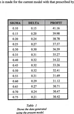
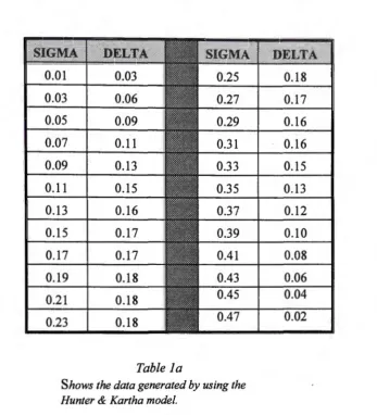
Discussion commences with a study of the relationship between the process standard deviation and the optimal value of 8 _{0 •}The data used is shown in Table 1 (the present model) and la ( Hunter&Kartha model). A graphical comparison is made for the current model with that prescribed by Hunter and Karth a.

SIGMA DELTA

0.10 0.15

0.15 0.20

0.20 0.24

0.25 0.27

0.30 0.30

0.35 0.31

0.40 0.32

0.45 0.32

0.50 0.32

0.55 0.31

0.60 0.29

0.65 0.27

0.70 0.24

0.75 0.21

Table I

Shows the data generated using the present model.

PROFIT ·

41.16

39.98

(9)

.. SIG-MA ··· <<DELl.'A SIGMA·

0.01 0.03 0.25

0.03 0.06 0.27

0.05 0.09 0.29

0.07 0.11 0.31

0.09 0.13 0.33

0.11 0.15 0.35

0.13 0.16 0.37

0.15 0.17 0.39

0.17 0.17 0.41

0.19 0.18 0.43

0.21 0.18 0.45

0.23 0.18 0.47

Table la

Shows the data generated by using the

Hunter & Kartha model.

DELTA

0.18

0.17

0.16

0.15

0.13

0.12

0.10

0.08

0.06 0.04

0.02

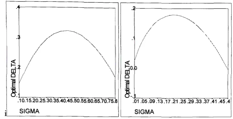
The optimal values of 8 (8 _{0 )}plotted against different values of cr ( keeping A, B,

a and e constant at A=67, B=O.SA, a=O.l, e=55)) are shown in Figure 2a. Several

observations are worth noting. As is clearly shown, a single optimal 8 value arises

from two distinct cr's. Figure 2b illustrates the same phenomena for the Hunter &

(10)

.

/ _ __.--·-·--·---.. ..

"

I

/

'"

,

~

I '\

.-

/

\

p / \

m·~

/

\

0 / \

~ I ,

~-

_{_}_.,..1o_~._{1-:-::5,....,}_._2-,.-0.~25~_{_3}_,....,_o~_._3-5_.~₄₀_~_.4-5~_._50-_.5~5~.6-o_.~_65~.1_-_0~_._1--15.a

SIGMA

Figure 2a

Shows the optimal delta values for sigma rangingfrom 0.1to0.8.

The results were obtained using present model.

~

cdo.o 0

~

~-.

l'--.~~~~~~~~~--.---l .01 .05.09.13.17.21 .25.29.33.37.41 .45.4

SIGMA

Figure 2b Shows the optimal delta values

for sigma ranging from 0.01 to 0.5.

The results were obtained using Hunter&Kartha model.

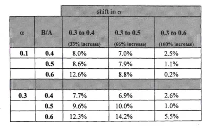
The second observation concerns the effect of various combinations of a,

the ratio between A and B and the percentage increase in cr on the optimal value

of

o.

This is illustrated in Table 2, showing the percentage change in optimal &

due to a shift in cr. The chosen values for a are 0.1 and 0.3, and for B/A are 0.4,

0.5 and 0.6. Smaller shifts in cr (33% increase) cause nearly the same change in

optimal

o

as a shift by 66%. If the process standard deviation shifts by 100% the optimal setting of proc~ss target is not significantly affected. The bigger the ratio

(11)

0.1 0.4 8.0% 7.0% 2.5%

0.5

8.6% 7.9% 1.1%

0.6 12.6% 8.8% 0.2%

0.3

0.4 7.7% 6.9% 2.6%

0.5

9.6% 10.0% 1.0%

0.6 12.3% 14.2% 5.5%

Table 2

Shows the percentage change in optimal delta due to 33%, 66%, and 100% change in er , where the distance between L and L ₀

increases from 0. 1 to 0. 3 and the ratio between A and B is equal to 0. 4,

0.5 and0.6.

It should be pointed out that the behaviour of cr in relation to 8 0 in Figure

(12)

.

. 3 Optimal DEL TA

.2

665462 60 58 PROFIT 5654

Figure 3

.4

SIGMA

.8

Shows the relationship between the optimal delta, the process standard deviation (ranging.from 0.1 to 0.8) and the maximum profit.

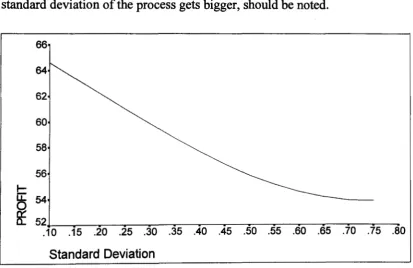
It is to be expected that an increase in sigma leads to a decrease in profit. This is shown clearly in Figure 4. The flatness of the optimal profit curve as the

standard deviation of the process gets bigger, should be noted.

66

64

62

60

58

56

I-~

54

0...: 52.l---..----~~~~~---=---..-::----=-~:---=----:~~-;;---::-;;:---~~

.10 .15 .20 .25 .30 .35 .40 .45 .50 .55 .60 .65 . 70 . 75 .80

Standard Deviation

Figure 4

(13)

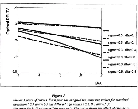
Figure 5 illustrates the effect of change in the ratio BIA on the optimal

process setting. It should be observed that for small

a (

in this case 0.1) the

optimal target setting seems to be approximately constant regardless of changes in

BIA or the standard deviation of the process. Note that the result obtained from

figure 2 is also clearly visible in Figure 5 .

~

_,

w

Q

~

a

0 . 4

.3

-

sigma=0.3, alfa=0.1

.2

sigma=0.6, alfa=0.1

-

sigma=0.3, alfa=0.3

.1 sigma=O. 6, alfa=O. 3

-

sigma=O. 3, alfa=O. 5

0.0._~~~~---~~~----~~~~----~~~~~ sigma=0.6, alfa=0.5

.3 .4 .5 .6 .7

8/A

Figure 5

Shows 3 pairs of curves. Each pair has assigned the same two values for standard deviation ( 0.3 and 0. 6) but different a/fa values ( 0.1, 0. 3 and 0. 5);

the same for both curves within each pair. The graph shows the effect of change in the ratio between A and B on the optimal target setting

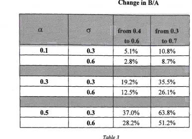
More precise analysis of the relation between the optimal target value of

the process and BIA is shown in Table 3, which illustrates the percentage change in

o

₀ due to change in pricing policy. It can be observed is that for relatively small a., if cr increases by I 00% then even a large increase in the ratio between A and B has

(14)

Change in B/ A

0.6 51.2%

Table 3

Shows the procentage change in optimal process setting due to change

in the ratio B to A. The distance between L and L ₀varies from 0. 1 to 0. 5, the process standard deviation shifts from 0.3 to 0.6 and BIA changes from 0.4 to 0.6 and from 0.3 to 0. 7.

The further L ₀ is from L (i.e. the larger the a) the bigger the effect of B/ A on optimal C3. These changes will be larger for smaller

a.

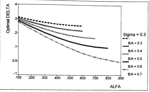
Figure 6 illustrates the result of relaxing or tightening the distance between L and L ₀ on the optimal solution. An increase in a reduces the value of the optimal () i.e. brings it closer to L _{0 •}This effect is more significant for small

(15)

<( .4

I-_J

w

0 (ij

E ~

c..

0 _.2

Sigma= 0.3

--·

_B/A

₌

_0.3

.1

-B/A = 0.4 I I 111

0.0

BIA= 0.6 -.1 _{-:-:-~~..--~~..--~~...--~~--~---..--~---...-~--.~~---J} _B/A

₌

_0.7

.100 .200 .300 .400 .500 .600 .700 .800 .900

ALFA

Figure 6

Shows curves of optimal delta values against values of a/fa for sigma= 0.3 and BIA from 0.3 to 0. 7.

5. CONCLUDING REMARKS

In this report the problem of selecting an optimal process mean in the

presence of'top-up' and 'give-away' has been defined and analysed.

The dependencies between the process parameters and the optimal value have been

described.

The results would seem to indicate that even if the process variance

deteriorates there is little gain in adjusting the mean per se but more appropriate strategy would be to concentrate on reducing variability as this increase will

diminish profit per item. Furthermore, if there is an increase in a., which would

likely be accompanied by a decrease in B (i.e. the ratio BIA will decrease) then

(16)

References

Bettes, D. C. (1962), "Finding an Optimum Target Value in Relation to a Fixed

Lower Limit and an Arbitrary Upper Limit," Applied Statistics, Vol.11,

pp.202-210.

Bisgaard, S.; Hunter, W. G. & Pallesen, L. ( 1987 ), "Economic Selection of

Quality of Manufactured Product," Technometrics, Vol. 26, pp.9-18.

Boucher T. 0. & Jafari, M.A. ( 1991 ), "The Optimum Target Value for Single

Filling Operations with Quality Sampling Plans," Journal of Quality Technology,

Vol.23, No.I, pp.44-47.