TUC: Time-sensitive and Modular Analysis
of Anonymous Communication
Michael Backes
Praveen Manoharan
Esfandiar Mohammadi
CISPA, Saarland University, Germany
[email protected]
[email protected]
[email protected]
February 12, 2014
Abstract
The anonymous communication protocol Tor constitutes the most widely deployed technology for providing anonymity for user communication over the Internet. Several frameworks have been proposed that show strong anonymity guarantees for such protocols; none of these frameworks, however, are capable of modeling the class of traffic-related timing attacks against Tor, such as traffic correlation and website fingerprinting.
Contents
1 Introduction 3
2 Related Work 3
3 Time-sensitive Network Model 4
3.1 Execution . . . 5
3.1.1 Machines & Session Identifiers . . . 5
3.1.2 Environment and Adversary . . . 6
3.1.3 Timing . . . 7
3.1.4 Communication Model . . . 8
3.1.5 Consistency Enforcing Scheduling . . . 10
3.1.6 Activation strategies . . . 11
3.1.7 Shared Memory . . . 11
3.1.8 Compromisation . . . 12
3.1.9 Runtime Bounds . . . 13
3.1.10 Discussion . . . 14
3.2 Properties ofEXEC . . . 15
3.2.1 Simplified activation strategy . . . 15
3.2.2 Internal Simulation of Multiple Machines . . . 16
3.3 Protocols . . . 18
3.3.1 Composition . . . 18
3.4 Ideal Functionalities . . . 19
3.4.1 Central vs. Distributed Ideal Functionalities . . . 20
4 Secure Realization 21 4.1 Security Definition . . . 21
4.2 Properties of Secure Realization . . . 22
4.2.1 Completeness of the Dummy Adversary . . . 22
4.2.2 Composition Theorem . . . 25
4.2.3 Joint State Theorem . . . 25
5 Time Sensitive Analysis of the Onion Routing Protocol 27 5.1 The Onion Routing Protocol . . . 27
5.1.1 User inputs . . . 29
5.1.2 Network Messages . . . 29
5.2 Time-sensitive Abstraction of OR . . . 30
5.2.1 Review ofFor . . . 31
5.2.2 Our Modifications toFor . . . 33
5.3 Abstracting Tor in TUC . . . 34
5.3.1 Assumptions . . . 34
5.3.2 Secure Realization . . . 37
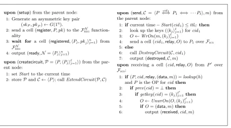
5.4 A User Interface: the Wrapper Πwor . . . 40
6 Timing Attacks in TUC 41 6.1 The Set-Up . . . 41
6.2 Mounting Attacks that use Timing Features . . . 41
7 Countermeasure against Website Fingerprinting 44
1
Introduction
Anonymous communication protocols, as provided by the Tor network [53], are an increasingly popular way for users to improve their privacy by hiding their location, i.e., their IP address. The Tor network is currently used by hundreds of thousands of users around the world [52].
In order to precisely understand the anonymity guarantees provided by Tor, several rigorous analyses have been conducted [2, 9, 21, 51, 3, 22], which show strong anonymity guarantees for the onion routing protocol used by Tor; however, all of these analyses abstract from network-level timing attacks, such as traffic correlation or website fingerprinting, which arguably form the most important class of attacks against Tor’s anonymity guarantees [14, 19, 43, 31, 23, 30, 41, 44, 46, 47, 55, 32]. One of the main obstacles in including such time-sensitive attacks into a rigorous analysis is the lack of a communication model that enables a composable security analysis of complex protocols against time-sensitive adversaries.
In this paper, we follow the successful line of research on simulation-based composable security, started with Goldreich et al. [25] and put forward by [6, 12, 16, 28, 39, 42], which enable a composable security analysis of complex cryptographic protocols.
Contribution. In this work, we present TUC: the first framework that allows for rigorously proving strong anonymity guarantees in the presence of time-sensitive adversaries that mount traffic-related timing attacks. TUC incorporates a comprehensive notion of time in an asynchronous communication model with sequential activation, while offering strong compositionality properties for security proofs. In particular, TUC is based on a modified version of GNUC [28], which is one of the recent pieces of work [12, 39] that address many of the problems faced by earlier designs for simulation-based security frameworks [11].
We discuss the modifications to the communication model of GNUC in order to adequately account for time, and we show solutions for problems that occur when handling time-sensitive interaction between different parties over the network. In particular, we discuss that previous frameworks inherently are not suited for modeling time-sensitive asynchronous communication because they allow unrestricted activation orders: it might, e.g., happen that a message that was sent in the past (over a direct connection) arrives after a time-out mechanism already closed a port, only because the sending party was not activated early enough. We propose a remedy by only allowing consistency enforcing activation orders, which enforce that all parties receive all messages at the correct time. It turns out that all consistency enforcing activation orders are equivalent. As a result, we fix the activation order and thereby, in contrast to previous work, neither the environment nor the adversary has to learn any unrealistic information about activation requests. We show that valued properties, such as the joint state theorem anduniversal composability, hold in our time-sensitive framework as well.
Finally, we apply TUC to the onion routing protocol that underlies Tor, and we show how traffic-related timing attacks, such as inter-packet delay, traffic watermarking, and website fingerprinting at-tacks, can be mounted by an adversary in TUC. Next, we propose a countermeasure against website fingerprinting attacks and utilize TUC to provek-recipient anonymity guarantees for this countermea-sure.
Outline. Section 2 discusses related work. Section 3 introduces the time-sensitive TUC framework, and presents the activation order independence of TUC. Section 4 then introduces the notion of secure realization into this time sensitive communication model and shows that classic results of composable security are preserved in the time sensitive setting. In Section 6, we discuss how known traffic-related timing attacks on Tor can be represented in TUC. Moreover, we provide a countermeasure against website fingerprinting attacks and prove it secure in TUC.
2
Related Work
Some protocols, such as the onion routing protocol, are inherently insecure against global adversaries, but provide guarantees against partially global adversaries, which might only control servers or the user’s links (like ISPs), and are useful in practice. Such systems cannot always be properly analyzed in time-insensitive frameworks [6, 12, 16, 28, 39, 42] because in these frameworks partially global adversaries are too weak: they cannot measure time-sensitive features, such as measure inter-packet delay or throughput per time interval, and they thus can also not measure effects of some active attacks, such as traffic watermarking or slowing down certain parties by mounting denial-of-service attacks. Since TUC enables the adversary to measure time-sensitive features, this family of attacks can be mounted by an adversary in TUC; thus, TUC is better suited for analyzing such weaker adversary scenarios.
This work contributes to the successful line of work on simulation-based universal composability frameworks [6, 12, 16, 28, 39, 42]. These frameworks allow for a composable analysis of large and complex multi-party protocols, where the security of the whole protocol is derived from the security analysis of the sub-protocols of which it is composed. We chose to base our TUC framework on the GNUC framework by Hofheinz and Shoup [28]. While GNUC is not as general as other frameworks due to its strict poly-time notion and its tree-like structure of party-structure, it has the advantage that a composed ideal poly-time protocol implies a composed real poly-time protocol due to its strict polynomial-time notion [28, Section 11.8], and simplifies the proof of the composition theorem and thereby also our extension due to its simple party-structure. We are, however, confident that the main mechanisms for introducing our comprehensive notion of time, including time-sensitive adversaries, can also be applied to other frameworks, such as the RSIM[6], IITM [39], and UC [12] framework.
Previous work on synchronous communication granting protocol parties the capability to measure time or to proceed round-wise in order to enable proofs about properties, such as guaranteed termination or input termination [34, 1, 16, 10, 35, 45, 49]. Such approaches, however, do not grant the adversary the capability to measure the time at which a message arrives.
Modeling timing attacks in synchronous frameworks might be possible, assuming very fast rounds and thus highly synchronized clocks, (in the order of milliseconds), but such an approach has two severe technical limitations: first, highly synchronized clocks can seldom be assumed in practice, in particular not for commodity hardware; second, such an attempt would technically only result in guarantees for protocols with highly synchronized clocks but not for protocols with loosely synchronized or unsynchro-nized clocks, while traffic-related timing attacks solely depends on the adversary’s clock and not on the protocol parties’ clocks. TUC grants the adversary access to a precise clock, independent of the parties’ clocks.
Networks of timed automata are well studied. However, they are seldom used for cryptographic purposes since timed automata are not as expressive as Turing machines. Thus, networks of timed automata are not sufficiently expressive for the analysis of cryptographic protocols. In particular, an adversary represented by a timed automata would be too weak.
There has been work on the time sensitive analysis of Dolev-Yao style abstracted cryptographic protocols using timed automata [7, 15, 33, 38, 37, 40]. However, this line of work analyzes Dolev-Yao style abstractions and therefore does not offer the full generality of networks of Turing machines.
3
Time-sensitive Network Model
In this section we present TUC, the first simulation-based composability framework that considers a time-sensitive adversary. TUC builds upon previous asynchronous simulation-based frameworks, such as GNUC [28] and the framework by Unruh [54], but fundamentally extends these frameworks by incorpo-rating a notion of time while preserving the highly desired properties such as universal composability
A general overview. We introduce time by capturing via a timer the current global time for every machine in the network. Whenever a machine is activated, its timer is updated based on the number of steps done by the machine and the speed of it. The speed of a machine is either predetermined if it already existed at initialization, or is determined by the protocol that it executes if the machine is created during runtime. Furthermore, we require that the actual local time experienced by each machine is given by a strictly monotonically increasing function of its current global time, thereby modeling unsynchronized clocks.
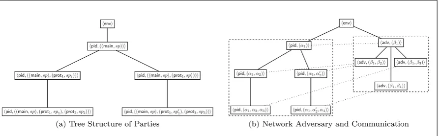
hpid,((main, sp))i
hpid,((main, sp),(prot1, sp1))i
hpid,((main, sp),(prot1, sp1),(prot2, sp2))i
hpid,((main, sp),(prot1, sp01))i
hpid,((main, sp),(prot1, sp0 1),(prot3, sp3))i henvi
(a) Tree Structure of Parties
hpid,(α1)i
hpid,(α1, α2)i
hpid,(α1, α2, α3)i
hpid,(α1, α02)i
hpid,(α1, α02, α4)i henvi
hadv,(β1, β2)i hadv,(β1)i
hadv,(β1, β3)i
hadv,(β1, β4)i
(b) Network Adversary and Communication
Figure 1: The Network Model in TUC
achieve that no party receives messages from the future, we introduce a distinguished machine, called the execution. This execution basically manages the timer of each machine and the timely delivery of messages between machines.
The execution attaches to each message that is sent through the network atime-stamp, which is only visible to the execution. This time-stamp, loosely speaking, denotes the local time of the sending party when the message was sent.
The environment and the adversary might consist of several machines that work in parallel. A natural way of modeling this capability is to represent these environment and the adversary as a set of parallel machine. While such a model is more accurate, we decided for the sake simplicity to over-approximate this strength of the environment and the adversary by allowing both parties to make an arbitrary (but poly-bounded) amount of computation steps in one time-step.
As in GNUC, a protocol is formalized as a runtime library that assigns to each machine the program code to be executed by the respective machine and the speed of the machine that executes the code. We stress that a network has only one such runtime library, i.e. one protocol.
3.1
Execution
The whole network is run inside single a machine we call execution (EXEC). The execution runs all parties in the network as sub-machines, delivers messages between these sub-machines, and maintains a timer for every sub-machine. We define the output ofEXEC as the output of the environmentEnv
after observing the communication between the involved parties. We capture this output by introducing a random variable.
Definition 1. The execution EXEC is a probabilistic, poly-time Turing Machine which receives the se-curity parameter η and outputs a value in {0,1}. EXECη(Π,A,Env) denotes the output of Env after
EXEC ran the network of machines running protocols in Π together with the network adversaryA and the environmentEnv. EXEC stops wheneverEnv halts and outputs a bit.
We first describe the single aspects of the executionEXECin the subsequent subsections, and at the end of this section we present the full description ofEXECin Figure 8.
3.1.1 Machines & Session Identifiers
In order to adequately represent complex protocols in our model, we adopt the notion of protocol machines from GNUC [28].1 Each partyP that participates in network communication is represented
by a tree of machines, each of which provides the sub-protocols used byP. This tree structure simplifies the substitution operation, which is used in the composition theorem (presented in Section 3.3.1). Our definition of a party is in line with what is presented as a structured system of interactive machines presented in [28, Section 3].
Each machineM in the network is identified by a uniquemachine ID idM. This machine ID consists
of a party identifier pidM and a session identifier sidM: idM = hpidM,sidMi. The session identifier 1Currently, our framework uses Turing machines as a machine model, but for analyzing timing leakage of algorithms
sid= (α1, . . . , αk) consists of theparent session identifier (α1, . . . , αk−1), the protocol nameprotNAME,
some session parameters sp, and the role: αk = (protNAME, sp,role). The protocol name is used to
determine the code executed by the respective machine, as detailed in Section 3.3.
Definition 2. The machine ID idM of a machine M is a tuple idM = hpidM,sidMi, where pid is
the party identifier and sid = (α1, . . . , αk) the session identifier of M. The last component of αk =
(protNAME, sp,role)is the basename ofM, whereprotNAMEspecifies protocol nameexecuted byM,sp
contains session parameters, androlespecifies the role in the protocol, e.g., client or server. The machine ID is unique to each machine.
Given such machine IDsidM, we define a party as a collection of machines{M1, . . . , Ml} such that
each machineMi has the same party identifierpidMi and the session identifiers of all machines induce a
tree, if the parent session identifier of each machine is the session identifier of another machine (except for the root).
Definition 3. A partyP is a collection of machines{M1, . . . , Ml} with following properties:
P1 : ∀i, j∈ {1, . . . , j}:pidMi =pidMj
P2 : ∃!M ∈ {M1, . . . , Ml}:sidM = (α)(called rootof P)
P3 : ∀Mj ∈ {M1, . . . , Ml} \ {M},∃Mi ∈ {M1, . . . , Ml} : sidMj is a one-step extension of sidMi, i.e. sidMi= (α1, . . . , αk−1)andsidMj = (α1, . . . , αk)
By Definition 2 and 3, the set of machines inside a partyP put up a a tree, given we understand each session ID as a node in a graph and have an edge between session IDs that are one-step extensions of each other.
Corollary 1. A partyP consists of a tree of machines.
Accordingly we will occasionally denote machines in such a machine-tree as nodes, and, given a pair of machinesMi andMj satisfying propertyP3, we callMi parent ofMj, andMj child ofMi.
As we will discuss in Section 3.1.4, we restrict communication between machines to communication between parent-children pairs, and machines that are so-calledpeers: a peer is a machine with the same protocol nameprotNAMEand the same session parameterspfor a basename (protNAME, sp,role).
Definition 4. Two machines M and M0 with the basenames (protNAMEM, spM,roleM) and
(protNAMEM0, spM0,roleM0) are peers if pidM 6= pidM0 and they both have the same protocol name
protNAMEM =protNAMEM0 and the same session parameterspM =spM0.
This formalization follows the intuition that a partyP represents the protocol stack executed on a real world machine, and network communication is done between sub-processes running the same protocol-code.2
We adopt all of the constraints listed in [28, Section 4,5] that ensure that each party indeed consists of a tree of machines and that each machine can only communicate with its parent, its children and its peers.
Inside a party, a machine in the machine tree can create new machines as children by sending a message to the yet non-existent machine. The execution then checks whether the message sent induces a valid extension – where validity is defined by the protocol used in the network, see Section 3.3 – of the machine tree and creates the new machine.
3.1.2 Environment and Adversary
Influences to network communication outside of the regular parties are traditionally captured in two special parties: the environment represents user behavior, operating systems or other entities that control the actions of the network parties, while the adversary represents adversarial behavior in the network.
Definition 5. The network adversary A is the unique party with party identifier pidA = adv. The
environmentEnv consists of only one machine with machine ID idEnv=henvi and is parent of all root machines of parties in the network.
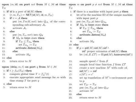
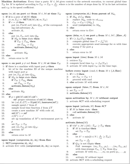
Initialization: All input tapes are set to empty, all timer-variables are set to the initial value and no links are compromised.
Machine Activation: Every time a machine M ∈ Mgives control to the network execution, to current global timeTM forM is updated according to
TM :=TM +
n cM
,
wherenis the number of steps done byM in its last activation andcM is its speed.
upon input (time)fromM ∈ M 1: retrieveTM
2: compute local timetM :=fM(TM)
3: activateM with inputtM on the time tape
before every input(cmd, t)fromM ∈ {A,Env} 1: if t >0then
2: setTM :=TM +t
3: proceed with cmd
4: elseactivateM witherror
Figure 2: Timing and Initialization in EXEC with machine set M, where fM is the M0s local time
function andfM =idforM ∈ {Env,A}
Similarly to the other parties, A consists of a machine-tree, where A has a sub-adversary for each basename in the network. Each of these sub-adversaries receives intercepted messages from the network originating from machines with the respective basename. The distributed design of the adversary allows us to formulate the construction for the composition theorem in Section 4.2.2 in a much simpler way. The tree-structure of the adversary is depicted in Figure 1b.
3.1.3 Timing
We finally extend the basic communication model presented in the previous sections to include time. We achieve this by attaching a timer to each machine in the network and by utilizing the executionEXECto maintain these timers. In order to allow un-synchronized clocks between network parties, we introduce local-time functions, which transform the timer’s value to the local time experienced by each machines. We achieve time-consistency for messages exchanged between machines by introducing time-stamps for these messages. The executionEXECutilizes these time-stamps for a timely delivery of messages to the recipient.
We introduce time into our model by assigning a timer to every machine in the system.
Definition 6. The timerTM ∈Qof a machineM is a rational-valued variable associated withM that
is maintained by the execution.
The timerTM is initialized to 0 at the beginning of the execution. TM records the current global time
ofM and is updated every timeM returns control to the execution. How muchTM is updated depends
on the speed ofM. Each machine has a different speed. Except for the environment and the adversary, the speed of each machine M is characterized by a speed coefficient cM, which specifies how many
computation stepsM does per time unit. Hence, for the timerTM ofM we have
TM :=TM +
n cM
wherenis the number of stepsM did in its last activation.
The poly-time notion we use in our communication model (see Section 3.1.9) necessitates that a machine makes a polynomially bounded number of steps per time unit: a machine with an exponential speed coefficient would not be able to meaningfully progress in time as each machine in our network model is restricted to at most a polynomial number of computation steps per activation. Hence, we require the speed coefficients be polynomials.
Definition 7. The speed coefficient of a machine M specifies the number of computation steps that
M can perform per unit time. The speed coefficient is a polynomialcM ∈N[X]. Whenever M returns
control to the execution,TM is updated byTM :=TM +cMn(η) where nis the number of steps M did in
its last activation andη is the security parameter.
request to the execution. EXECthen computes the local time ofM by applyingM’s local time function fM to its current global timeTM. The execution and the simulating machine in the internal simulation
lemma (Lemma 2) need to be able to efficiently compute and invert the local time; thus, we require that the local time function be efficiently computable and invertible function.
Definition 8. Thelocal time functionfM :Q→QofM is a strictly monotonically increasing, efficiently
computable and efficiently invertible function that transforms the value ofTM toM’s local timefM(TM).
We require the local time function to be invertible as EXEC needs to invert the local time function in order to process delayed message sending, which is an option for protocol machines in the network and will be required in our constructions in Section 7. We make a worst case assumption and define the local time function of the environmentEnvand the network adversaryAto be the identity function(see Figure 2).
Speed coefficients and local time functions are fixed once the machine is spawned. Formally, the speed coefficient and the local time function depend on the protocol, the session parameter, the role, and the party ID. In order to assign speed coefficients to dynamically created machines, we require the protocol Π to determine for each basename not only the code to be executed but also a distribution over the speed coefficients and a distribution over local time functions (see Definition 21). The execution draws the speed coefficients from these distributions whenever a new machines is created during runtime.
In the real world, the environment and the adversary might consist of several machines that work in parallel. A natural way of modeling this strength is to represent the environment and the adversary as a set of parallel machines. While such a model is more accurate, for the sake of simplifying proofs, we abstract this strength of the environment and the adversary by allowing both parties to make an arbitrary amount of computation steps per unit time.3
Definition 9. A machine M is timeless if it does not have a speed coefficient and M itself tells the execution the time-difference by which its timer increases next time it returns control to the execution.
Note that by the notion of poly-time we introduce in Section 3.1.9 this still restricts both to at most a polynomial number of computation steps (in the security parameterη) per activation.
3.1.4 Communication Model
We differentiate between inner party communication between parent and children nodes inside a party and network communication between peers using a notion ofports: we distinguish betweenenvironment,
subroutine, andnetwork port. Figure 1b illustrates this with thick lines for inner party communication and dashed lines for network communication.
Definition 10. Aportpof a machineM is a set of one input tapepinand one output tapepout that is
used by the execution to pass information to M. Each machine has one environment portsid(M).Env, a network portsid(M)net and a set of subroutine portsSM.
For communication over the network, M sends its messages over its network port, addressing the recipient using the recipient’s machine id. All incoming messages are received throughM’s network port as well. A machineM can only send messages over the network to another machineM0 if eitherM0 is a peer ofM or M0 is the network adversary.
M uses it environment portsid(M).Envto communicate with its parent, or ifM is a root node, with the environment. The set of subroutine portsSM contains a unique port for each child ofM. In caseM
wants to create a new machineM0 as a child,M creates a new portp0 in S and addresses M0 through
this port. EXECthen recognizes thatp0 is not in use yet and creates a new machineM0, as detailed in
Figure 3.
Inner party ports follow the naming conventionpid.sid1.sid2. Herepidis the process ID of the party,
sid1 is the session ID of the parent node Mp, andsid2 the session ID of the child nodeMc. Note that
Mc communicates to its parent via its environment ports. The execution therefore makes an implicit
port translation between environment ports of children nodes and inner party communication ports as defined above. Through this, we realize a variant of what is introduced asCaller ID Translation in [28, Section 4]. The methods used for message passing insideEXECare presented in Figure 3.
3For the completeness of the dummy adversary, the adversary needs to be able to forward message in a way that
upon (m,id) on port net from M ∈ M at time
TM
1: if idis a peer ofid(M)then
2: (r, m, Tm)←NET(id(M),id, m, TM)
3: if r=Athen
4: put (m, T mM, net) into QAi of the
corre-sponding sub-adversaryAi.
5: activateAi.
6: else
7: put (m, Tm, net) intoQid
8: if Mid inlistenstatethen
9: if TM ≤T˜Mid then
10: set ˜TMid :=TM
11: activate listen(Mid)
12: else
13: activateMid
14: else
15: return error to M
upon(delay, m, t)on port q fromM∈ M
1: if t≥fM(TM)then
2: compute global timeT =fM−1(t)
3: execute appropriate send message for mwith time stamp T for portq
4: else
5: return error to M
upon m on port p6=net from M ∈ M at time
TM
1: if there is a machine with input portpthen 2: letidbe the machine ID of the unique machine
with input portp
3: put (m, TM, p) intoQMid
4: if Mid inlistenstatethen
5: if TM ≤T˜Mid then
6: set ˜TMid :=TM
7: activate listen(Mid)
8: else
9: activateMid
10: else
11: if p=pid(M).sid(M).sid0∧
sid0proper extension ofsid(M)then 12: let (cd,S,LT) = Π(pid(M),basename(sid0))
13: sample speedc0fromS
14: sample local time functionf fromLT 15: create a new machineM0 with codecd,
16: sid(M0) :=sid0
17: c(M0) :=c0
18: set up translation ofM0’s environment port top
19: setTM0 =TM
20: put (m, TM, p) intoQM0
21: activateM0
22: else
23: return error toM
Figure 3: Communication methods inEXEC with machine setMand protocol Π
For the case that a machine waits for incoming messages, we introduce a listen-command: (listen, T). As soon as this command is sent, the execution EXEC will not activate these machines until either (i) they receive a message, or (ii), they can no longer receive a message before time T. The machines also have the possibility to setT =∞the machines then will not be activated unless they receive a message. Once the machine is activated, their timer is also updated, either to the time-stamp of the received message, orT if the machine is activated without a message.
Timing in communication. In contrast to other sequential activation models, messages in TUC are not directly delivered to the recipient because there might be another message from a yet not activated machine that has to arrive earlier. More formally, if M sends a message to M0 and TM > TM0, then
the message obviously should not reach M0 until TM0 ≥TM. The execution remedies this problem by
utilizing time stamps.
Definition 11. The time stampof a messagem sent by a machineM is the updated value of the timer
TM at the point when M sends the message.
The execution attaches this time-stamp to each message before it is sent to the recipient. On the recipient’s end we use time-ordered queues, called input queues, which organize all messages that still need to be received, and release them once the recipient has progressed far enough in time. It is crucial that we deliver all messages at once; otherwise it is not clear how to internally simulate several machines (see the proof of Lemma 2).
Definition 12. The input queue QM of a machineM is a priority queue which receives all messages
directed to M as input and uses their time-stamp as the keys which are sorted. On request with a time-stampT,QM returns all messages with time-stamp Tm≤T.
When deliveringm,EXECputs the tuple (m, Tm, p) into the input queueQM0 ofM0. Herepdenotes
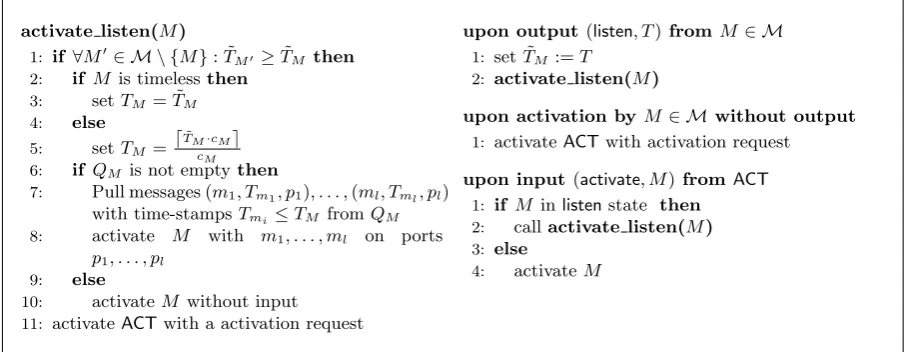
activate listen(M)
1: if ∀M0∈ M \ {M}: ˜TM0≥T˜M then
2: if M is timelessthen 3: setTM = ˜TM
4: else
5: setTM =d ˜ TM·cMe
cM
6: if QM is not emptythen
7: Pull messages (m1, Tm1, p1), . . . ,(ml, Tml, pl)
with time-stampsTmi ≤TM fromQM 8: activate M with m1, . . . , ml on ports
p1, . . . , pl
9: else
10: activateM without input
11: activateACTwith a activation request
upon output(listen, T) fromM∈ M 1: set ˜TM :=T
2: activate listen(M)
upon activation by M∈ Mwithout output 1: activateACTwith activation request
upon input (activate, M) fromACT
1: if M inlistenstate then
2: callactivate listen(M) 3: else
4: activateM
Figure 4: Activation order methods in EXECwith machine setMand activation strategyACT
them toM. In case there are several messages inQM0 that could be retrieved at timeTM0,QM0 simply
returns all of them. All methods involved in message passing are presented in Figure 3.
3.1.5 Consistency Enforcing Scheduling
Other simulation-based frameworks use a sequential activation model: machines in the network directly activate each other by sending messages and the environment or the adversary decides which machine is activated in case no messages. We call these decisions theactivation strategy. Keeping to this unrestricted sequential activation model, however, causes several problems as soon as time is introduced: messages from the past arrive at nodes which are already in the future or the activation order (which is usually represented by the adversary or the environment) can push machines arbitrarily far into the future. The example below shows how this can lead into problems with a timeout mechanism, assuming the adversary decides the activation order.
Example 1: Inconsistencies with unrestricted sequential activation strategies. Consider ma-chinesM and M0 which go into a timeout state if they do not receive a message up to some point in
timeT∗
1: Env repeatedly actives machine M throughA, which causes M to activate for one step and then
return to the listening state. This effectively pushes M to timeT > T∗the future.
2: M goes into the timeout state, as it did not receive any message until timeT∗
3: Env tells machine M0 to send a message toM at timeT0. Including processing the command, the
message is sent at timeT0
4: M receives a message from timeT0< T∗ at time T∗.
M now erroneously went into the timeout state, even thoughM0sent a message toM before the timeout
should have occurred.
We avoid such inconsistencies as follows: we introduce a special (listen, T) state for the machines in the network, in which they have to be in order to receive messages. Furthermore, we deviate slightly from the traditional sequential activation model by discarding activation commands that do not satisfy the following consistency enforcing property.
Definition 13 (Consistency Enforcing). An activation order of machines is consistency enforcing, if
∀M0 6=M : ˜TM ≤T˜M0 wheneverM is activated from the listening state. Here T˜M is the virtual time of
the machineM defined as follows:
• T˜M = min{T, Tm}, where Tm is the smallest time-stamp of a message in QM (or ∞ if no such
message exists), if M is in the(listen, T)state
• T˜M =TM, if M is not in the (listen, T)state
Upon activation with input (write, D, d, M, TM):
1: letD[Ti,∞]be the last version ofD 2: setD[Ti,TM]:=D[Ti,∞]
3: removeD[Ti,∞] 4: setD[TM,∞]:=d
5: return confirmation toM
Upon activation:
1: if there is an input (lookup, D, M, TM)then
2: put the request (lookup, D, M, TM) into the queueQL
3: letT∗be the smallest timer value inMMEM
4: while∃lookup requestsQLwith time stampT ≤T∗do
5: remove request (lookup, D0, M0, TM0) with smallest time stampTM0 fromQL
6: return data setD[Ti,Ti+1], TM ∈[Ti, Ti+1) to requesting partyM
Figure 5: The shared memory MEM
Corollary 2. Under consistency enforcing activation orders, whenever a machineM is activated from thelistenstate at timeT,M receives all messagesmwith time-stampTm≤T and any messages not yet
received were sent at a timeT0 > T.
3.1.6 Activation strategies
We need anactivation strategy to determine the machine to be activated next whenever a machine turns inactive after switching into thelistenstate. Under consistency enforcing activation orders, however, we cannot take the same approach as previous frameworks, in which the adversary decides the activation strategy: since the adversary is a time-sensitive component of the network and thus also affected by consistency enforcing activation order, the network can end up in a deadlock situation where all machines can either not be activated, or are stuck in the listen state. To avoid this problem we introduce the activation strategy as a sub-machine of the executionEXEC.
Definition 14. The activation strategy ACT is a probabilistic, poly-time TM, which, given the state of the network as input, determines the next machine to be activated.
ACT does not have a timer and implements the activation order based on the current state of the network. EXECenforces the consistency enforcing property be checking the required conditions whenever ACT wants to activate a machine. In Section 3.2.1, we show that all consistency enforcing activation orders are equivalent. The activation methods are depicted in Figure 4.
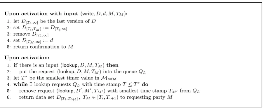
3.1.7 Shared Memory
As in other simulation-based framework, our goal is to analyze complex protocols by simplifying them to ideal functionalities with additional capabilities. We captures these capabilities in form of shared memory between all ideal peers in the network. Access to shared memory is granted via a special port through which parties can request read/write actions on the memory.
Definition 15. Ashared memoryMEM is a machine without a timer which, given the current state of the network, implements time-sensitive data exchange outside of message passing. The set of machines with access to MEMis denoted withMMEM.
MEM maintains every version D[T1,T2] of each data-set D with respect to time (organizing them
through time-intervals[T1, T2] between changes) and on request at timeT returns the versionD[Ti,Ti+1]
of data setD with T ∈[T1, Ti+1)
Similar to the activation orders, the concept shared memory causes consistency issues: For example, what happens if a party that lives in the past changes a data set a party living in the future already read (in the future)?
Example 2: Consistency issues in shared memory.
Consider two machinesM (living at timeTM) andM0 (living at timeTM0 < TM) which both access the
shared memoryMEMto read/modify a data-set d.
1: Env tellsM to readdfromMEM 2: M readsdfrom MEMat timeTM+δ 3: Env tellsM0 to modifydinMEM
4: M0 modifiesdin MEMat timeTM0+δ0 < TM +δ
M now has read the value ofdwhich is actually no longer correct, asM0modifieddin the past afterM
read it.
We solve these consistency issues by using a variant of consistency enforcing activation orders.
Definition 16. Shared memory access is consistency enforcing if a lookup requests (lookup, D, M, TM)
is only processed if∀M0∈ MMEM:TM0 ≥TM.
If this condition is not true, the shared memory puts the request together with its time stamp into a input queueQL, which sorts all unanswered requests by their time stamps. Upon every activation,MEM
checksQLfor unanswered lookup requests and retrieves the one with the smallest time stamp. MEMthen
checks the lookup request for validity (based on its time stamp), and processes it if it is. In caseMEM cannot process any lookup requests, it finishes the execution without sending a confirmation message. Figure 5 gives a possible pseudo-code implementation of a shared-memory unit in the time-sensitive network model.
As a consequence of consistency enforcing memory access we get Corollary 3 which ensures consistency of shared memory entries read by machines in the network.
Corollary 3. If a data setD is read by a party M from a consistency enforcing shared memory MEM
at timeT, then any changes toD will only happen at a point in time T0 ≥T.
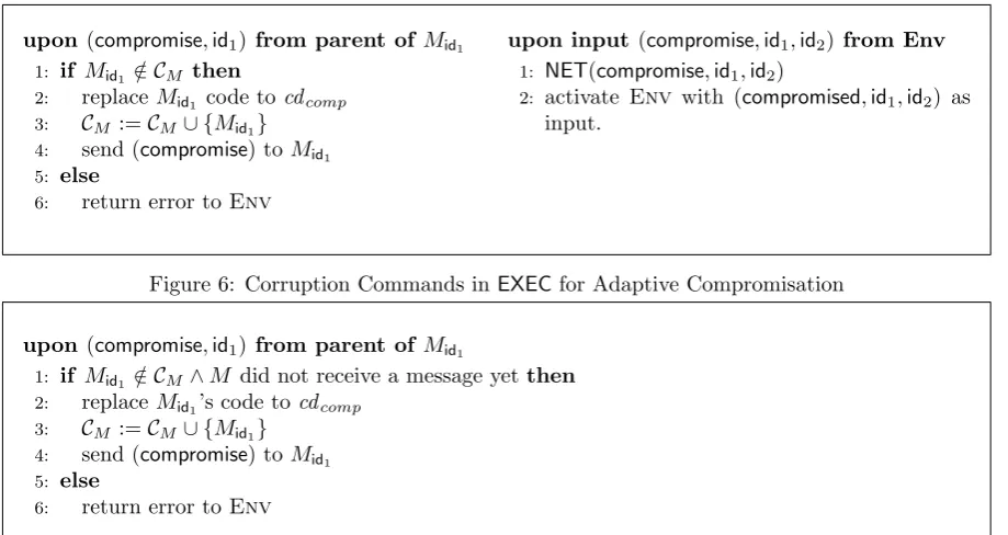
3.1.8 Compromisation
An important part in the analysis of protocols is accurately modeling adversarial capabilities, which includes restricting the adversary’s access to the network, as well as differentiating between active and passive adversaries.
Link corruption. Previous composability frameworks assume a global adversary which intercepts all messages sent between parties over the network. This is a necessity for realization proofs between protocols which do not inherently leak information to the adversary. However, in the special case of anonymous communication (AC) protocols, a global adversary poses a problem: Tor, e.g., is not secure against global adversaries [55, 47, 44, 14], it is not even designed to be secure against global adversaries. Previous work on the analysis of Tor shows how partial compromisation of the network can be modeled by introducing special network functionalities Fnet, which are used as a link between parties [2]. Fnet only leaks a message to the network adversary if the communication link they represent is compromised. To simplify the analysis, especially with regard to AC protocols, we assume an initially uncompro-mised network. The environmentEnv, however, can compromise network communication links between two machines by sending a compromise message to the executionEXECindicating which link should be compromised. Afterwards, any communication on the compromised link is forwarded to the adversary A(see Figure 6).
We assume that inner-party communication, i.e. communication between children and parent nodes inside a partyP, cannot be intercepted without compromising the party: a party models a system that resides at one physical location.
upon(compromise,id1)from parent of Mid1 1: if Mid1 ∈ C/ M then
2: replaceMid1 code tocdcomp 3: CM :=CM ∪ {Mid1}
4: send (compromise) toMid1 5: else
6: return error toEnv
upon input(compromise,id1,id2) from Env 1: NET(compromise,id1,id2)
2: activate Env with (compromised,id1,id2) as
input.
Figure 6: Corruption Commands inEXECfor Adaptive Compromisation
upon(compromise,id1)from parent of Mid1
1: if Mid1 ∈ C/ M∧M did not receive a message yetthen 2: replaceMid1’s code tocdcomp
3: CM :=CM ∪ {Mid1} 4: send (compromise) toMid1 5: else
6: return error toEnv
Figure 7: Machine Corruption inEXEC for Static Compromisation
Party corruption. The network machines themselves can also be completely compromised by the environment Env. Upon receiving a compromisation message compromise, EXEC replaces the code executed by the receiving machine M with the following code of a compromised machine cdcomp and
forwards the corruption message to M, which in turn responds with an answer toEnv containing the current state ofM and from then on is under full control of the adversary(see Fig. 6). cdcomp is defined
as follows: wheneverM receives a message, it is forwarded to the adversary, who in turn instructsM. Since the adversary is modeled as a network party, we cover passive as well as active adversaries: a passive adversary would simply forward all messages he intercepts, while an active adversary can send additional messages through the network as well as change intercepted messages.
The analysis of AC protocols usually differentiates between two important classes of Compromisation.
Definition 17. An execution allows for static compromisation if machines and communication links can only be compromised at initialization. It allow for adaptive compromisationif the environment can compromise even during run-time.
While the presentation of EXEC in Figure 8 works for the adaptive case, we need to make some changes for the static case: In the static case, a set of machines and links is already compromised at the beginning of the execution and corruption commands are no longer available for the environment during the execution.
Compromised machines however can still create new machines. These new machines should be com-promisable before they start to interact with the rest of the network. We therefore allow for a modified machine compromisation method in the static case, which only forwards thecompromisecommand if it is the first message the newly created machine receives (see Fig. 7).
3.1.9 Runtime Bounds
Correctly addressing polynomial runtime bounds for networks of machines has been a point of major debate in the literature [29]. We adopt the solution put forward in [28, Section 6] . We only give a high level idea of the notion of a probabilistic polynomial time network and refer to the GNUC paper for a thorough discussion [28, Section 6].
The IITM-model proposes a simpler notion of poly-time machines which is compatible with our communication model as well. As discussed in [28, Section 11.8] however, this notion does not imply poly-boundedness for the composition of poly-bounded machines, which the definition in GNUC does.
We require that each message sent through the network begins with the string 1η, where η is the
security parameter used in the execution. If a machine is activated without a message, it receives the string 1η on a special activation input port. This ensures that on any activation, the activated machine
Run-time of machines in the network is defined based on the length of the messages they exchange, i.e. theflow between machines. To this end we denote withfep(η) the flow from the environmentEnv
to protocol machines Π, withfea(η) the flow from Env to the adversary A, and with fap(η) the flow
fromAto Π.
We only consider environments which on each activation are polynomially bounded in their input and which additionally are well-behaved.
Definition 18. An environment Env is well-behaved if there is a polynomial p such that for every adversary and for all security parametersη,
fe(η) =fep(η) +fea(η)≤p(η)
With this, we can define probabilistic, poly-time protocols.
Definition 19. LetTΠ
η [Π,Env,A]denote the accumulated number of steps done by all machines running
Π. A protocol Π is probabilistic, poly time(PPT) if there exists a polynomial psuch that for all every well-behaved environmentsEnv,TΠ
η [Π,Env,A]can be bounded by
P r[TηΠ[Π,Env,A]> p(fep(η) +fea(η))]≤negl(η)
In order to get an overall poly-time execution, we also only allow bounded adversaries.
Definition 20. An adversary A is bounded for Π if A is time-bounded for Π, i.e. there exists a polynomialpsuch that for all well-behaved environments Env we have that
P r[TηA[Π,Env,A]> p(fep(η) +fea(η))]≤negl(η)
and ifAis flow-bounded forΠ, i.e. there exists a polynomialp0such that for all well behaved environments
P r[fap(η)> p0(fea(η))]≤negl(η)
With these restrictions we get an execution EXEC which overall uses a polynomial number of steps in the security parameterη.
Lemma 1. For all well-behaved environments Env, allPPTprotocols Π, all bounded adversariesAfor
Πand all inputsx∈ {0,1}p(η)the executionEXEC
η(Π,A,Env)is probabilistic polynomial time inη with
overwhelming probability.
The lemma follows, on the one hand, from Π and Abeing polynomially time-bounded in their in-coming flow (with overwhelming probability), A being flow bounded (with overwhelming probability), andEnv being well-behaved. On the other hand we have that EXEC only requires polynomial time to update the timers of each machine, compute their local time-functions, compute the input queues of each machine and check the condition for consistency enforcing activation orders. EXECtherefore overall only uses polynomial time.
Note that we also inherit the notion of invitations from GNUC. This technical artifact is sometimes required for the construction of the simulators in proofs of secure realization (see 4), which often cannot wait until they receive a message from the environment before they interact with protocol machines. For brevity we do not directly include them into our construction, but stress that their inclusion do not cause any problems with runtime bounds: invited messages do not count towards the flow we bound. But since only polynomially many invitations are generated, the overhead of invited messages can be polynomially bounded as well.
3.1.10 Discussion
In spite of consistency enforcing activation orders, TUC can be used to model asynchronous com-munication by protocols that do not use their local clock.4 Arbitrary networks delays for compromised
links can be modeled in TUC since the network adversary can arbitrarily delay a message.
Beside the advantage that asynchronous communication can be modeled by arbitrary activation strategies, another effect of (traditional) arbitrary activation strategies is that it can model, by not activating a machine, crashed nodes, but only if these machines would not have received any message (otherwise this message would activate them). Since this mechanism anyway only covers machines that would not have received any messages, we believe that such crashes should rather be explicitly modeled, i.e., in the same way as corruptions, and not via an activation strategy.
Encoding our approach in previous frameworks. It might be possible to wrap each machine M in the network in a local wrapperW that performs the same actions as the executionEXECin TUC.W would count the number of steps thatM performs and divides these steps by the speed of that party to calculateM’s current time. This wrapperW would for each outgoing message fromM add a timestamp and for each incoming remove the timestamp before forwarding it to the recipient. Moreover,W would order every incoming messages in a time-ordered input queue and only deliver those message to M for whichM already proceeded far enough in time.
Such a network of locally wrapped machinesW(M1), . . . , W(Mn), however, does not ensure the
consis-tency enforcing property for activation orders, i.e., allows inconsistent activation orders (see Example 1). Since consistency enforcing is a global property the local wrappersW would have to synchronize their timer information to find the next, eligible party and activate this party (by sending some dummy mes-sage). Although it might be possible to show that such an encoding is equivalent to our approach, we believe that it is more elegant and easier to understand to incorporate time-sensitive adversaries as done in TUC.
3.2
Properties of
EXEC
We present two properties which will be helpful for proving the security properties of TUC.
3.2.1 Simplified activation strategy
It turns out that under consistency enforcing all activation strategies are equivalent to the following activation strategy SAS, as long as no deadlocks occur: the next machine to be activated is selected based on each machine’s timerT by randomly selecting a machine with the lowest timer value.
Theorem 1. Let EXEC0k,S,t(Π,A,Env) denote the machine that executes EXECk(Π,A,Env) with the
activation strategy S. MoreoverEXEC0k,S,t(Π,A,Env)records the internal states of all machines in the execution after each step together with the global time in which that machine was during that state. After the execution finished,EXEC0k,S,t(Π,A,Env)outputs the sequence of all states of all machines (including
AandEnv) up to the timet. Letreach(S, t)denote the following property: the probability that for allA and allEnv and allx∈ {0,1}∗ inEXEC0
k,S,t(Π,A,Env)all machines reach a time > tis overwhelming
ink.
Let A be a (potentially timeless) machine and let S1, S2 be any two activation strategies, i.e., any
two machines that, given all the information that the executionEXEChas, (adaptively) determine which machine shall be activated next. For all sets of machinesP :={P1, . . . , Pn}(n∈N),S1is
indistinguish-able fromS2, i.e., for all points in timet∈Qand for all distinguisher machinesD there is a negligible
function such that:
reach(S1, t)andreach(S2, t) =⇒
Pr[b← hD|EXEC
0
η,S1,t(Π,A,Env)i:b= 1]
−Pr[b← hD|EXEC0η,S2,t(Π,A,Env)i:b= 1]
≤µ(η)
Proof. First, we prove the following statement.
4Even the slightly stronger setting in which each party uses its local clock, but the clocks are completely unsynchronized
Claim 1: For two activation strategies S1 and S2, EXEC0η,S1,t(Π,A,Env) is indistinguishable from
EXEC0η,S2,t(Π,A,Env) if and only if the sequence of results of alllisten-commands, i.e., the input message with which the respective machine is activated, is indistinguishable in both scenarios.
Proof of Claim 1. By the definition of EXEC all the information that A can observe is independent of the activation order except of the results of the pull-queries to the input queue QA. Hence, it is
indistinguishable whether the strategy S1 or S2 has been used. The reverse direction holds because
every machine can use the result from thelisten-command to distinguish the two settings. Let EXEC0η,S1,t,i(Π,A,Env) be the execution (with the activation strategy S1) that stops after the
ith activation of a machine that is in thelistenstate. LetEXEC0η,S2,t,i(Π,A,Env) be defined analogously.
We perform a proof by induction over the activation of machines that are in thelistenstate. Induction basis (i= 0): By Claim 1 the two activation strategies are indistinguishable.
Induction step (i >0): We know that for all i−1thlistenactivations the two activation strategies S1 andS2 are indistinguishable. Thus, the results of alli−1listen-commands are indistinguishable for
both activation strategiesS1 andS2. Thus, by Claim 1, it remains to show that also seeing the result of
theithlisten-command is indistinguishable.
Let M be the ith machine that is activated in the listenstate. If no machine sent a message to M since thei−1thlisten-command, the statement follows by induction hypothesis. Assume that at least one message has been send toM since thei−1thlistenactivation. LetT be the global time ofM when it issue thelisten-command. By consistency enforcing property of the activation order, we know that all machines are at least in timeT0 ≥T whenM is activated in itslistenstate for any activation strategy
S that lets all machines reach the (global) timeT. By the definition ofEXEC, we know that afterM is activated (upon alisten-command) no machine can send a message M that will get a timestamp ≤T. Hence, the input of thelistenactivation, i.e., the inputs from the input queueQM, are independent from
the activation strategy. Hence, by Claim 1, the statement follows.
Theorem 1 directly implies that the activation strategy SAS is indistinguishable from any other activation strategy as long as no deadlock occurs.
Corollary 4(SASis equivalent to all deadlock-free activation strategies). The activation strategySAS
is indistinguishable from any other, deadlock-free activation strategy(in the sense of Lemma 1).
3.2.2 Internal Simulation of Multiple Machines
Here we show that a finite numbernof timed machinesM1, . . . , Mnin our network can be simulated by a
single machineM∗which shows same behavior as thenseparate machines. While the internal simulation
is clearly not a problem ifM∗ is timeless (even if some of the simulated machines are timeless), this is
not clear for the case whereM∗ is a timed machine with a timer that automatically progresses in time
wheneverM∗ does a computation step.
The following lemma will allow us to simplify large parts of the theorems we show regarding the security definition we introduce in section 4.
Lemma 2. For any set of n timed machines M1, . . . , Mn in the network there exists a single timed
machinesM∗ which shows the same behavior asM1, . . . , Mn for consistency enforcing activation orders.
Proof. We construct and show thatM∗ sends the same messages asM1, . . . , Mn, together with the same
time-stamps, into the network.
Construction: We set the speed coefficient ofM∗toc
M∗=n·cM0+O(n), whereM0 ∈ {M1, . . . , Mn}
is the machine with the highest speed coefficient. The local time function of M∗ is the identity.5 This
allowsM∗ to do at least one computation with every internally simulated machine without progressing
in time further than M0 (since each simulated computation step also causes one computation step in
M∗).
M∗ inherits all ports of the machines it simulates. Thus all messages intended for the internal
machines are first received byM∗, who then forwards them appropriately.
In particular this implies thatM∗ has more than one network port: M∗ hasn network ports, each
of which are identified with the identifiers of M1, . . . , Mn. This is necessary sinceM∗ needs to be able
to differentiate between the recipients of messages coming intoM1, . . . , Mn and the senders of messages
going out ofM1, . . . , Mn. SinceEXECautomatically identifies network ports based in machine ID,
mes-sages targeted at machines insideM∗are automatically forwarded to M∗.
In principle,M∗simply emulates the network execution for the machines it simulates, managing message passing from the machines to the real executionEXECand the activation order. As shown in Lemma 1, M∗ can adopt the strategy of activating the machine with the lowest timer value.
In particular,M∗now works as follows: on regular activation,M∗simulates each machineM
1, . . . , Mn
for one computation step at a time, each time activating a machine M0 with the lowest timer T M0
(randomly choosing one if more than one machine is at time TM0). M∗ stops the simulation if all
machines with the lowest timer value are either in the listening state or returned control to the execution. M∗ sends each message sent out by the simulated machines using the delayed sending command (see
Figure 3), using the appropriate time-stamps.
M∗ performs idle steps until its own timer matches the lowest timer valueT0. Then,M∗ turns into
the listening state of the network port of machineMiif there is a machineMiatT0that is in the listening
state (randomly choosing one if there is more than one), or simply returning control toEXECotherwise. If activated from the listening state, M∗ automatically receives all messages on its ports with time-stamps smaller thanTM∗. These messages are forwarded to the message queues of the machines inside
M∗, with TM∗ as a time-stamp, and each machine is in turn activated for one computation step each.
M∗ then continues with the usual activation order as described above.
Upon a command (listen, T) from a party, M∗ computes the virtual time ˜T
M for each machine M
and handles the (listen, T) command asEXEC. M∗ can compute for a machineM the virtual time ˜T M
since it knows the speed coefficient ofM and the content of the input queue of M.
We show by induction over the activations ofM∗that M∗ shows the same behavior towards the rest of
the network asM1, . . . , Mn:
Activation 1: On initial activation, all timers are the initial value, and no machine is in the lis-tening state. M∗will in turn simulate each internal machine until all machines with the lowest timerT0
either sent a message or went into the listening state.
Due to our selection of the speed coefficient cM∗ ofM∗, we have that at this point TM∗ < T0, with
enough time for M∗ to forward all messages sent by the simulated machines using the delayed sending command, and turning into the listen state at timeT0. Since all messages until T0 were sent with the right time stamp, and the simulated machines are activated in the same order as they would have been activated from the execution (due to consistency enforcing scheduling), the behavior ofM∗is the same as the behavior of each single machineM1, . . . , Mn.
Activation i → i + 1: M∗ is either gets activated regularly or from a listening state. The
for-mer case is the same as for the initial activation above, hence we only consider the activation from the listening state.
Being activated from a listening state means there are machines with timer value TM∗ simulated in
M∗, which also are in the listening state. Due to consistency enforcing scheduling, each of these machines
receive all messages they would have received in the regular network as well (since all other machines in the network have progressed pastTM∗).
Messages forwarded to machines which are not in the listening state at timeTM∗correctly receive these
messages once they go into the listening state. The potentially changed time-stamp of these messages insideM∗ does not influence the behavior of each machine as they do not receive the time-stamp of the message (it is only used by the network execution, which here is simulated byM∗).
Hence all machines receive the same messages as in the regular network, at the same points in time, and thus will also produce the same output messages, at the same points in time, as well.
We stress that Lemma 2 does not enforce the tree-restrictions of machines inside a party defined in Section 3.1.1. One should still mind these restrictions if composition is to be used on together with above construction.
As a corollary, we can show that a timeless machine can also internally simulate other timeless machines.
Corollary 5. For any set of n machines M1, . . . , Mn in the network there exists a single timeless
machinesM∗ which shows the same behavior asM
Proof. The simulator is exactly constructed as in the proof of Lemma 2 except that the activation is slightly modified. All timed machines are only activated once in one point in time, but timeless machines are activated (in a round-robin manner) as often as they stay in that point in time. Moreover, if a simulated timeless machineMi sends a message at timetand no other machine wants to perform a
computation,M∗performs a (listen, t) command, wheretis the minimal time of the next timed machine
that could perform a step and a message that shall be sent or.
3.3
Protocols
A protocol is a runtime library that assigns to each basename (i.e., protocol name, session parameter, and role) used in session IDs the respective program code to be executed by the respective machine and the speed of the machine that executes the code. Recall that a network has only one such runtime library, i.e., one protocol. This library assigns to all parties the respective code and speed for the single machines.
In the definition below, we denote withDist(X)⊂X →[0,1] the set of distributions over the natural numbers (without 0). Moreover, we denote withMonA→B the set of strictly monotic functions from A
toB and withD the set of machine IDs.
Definition 21. For a set P of party IDs and a set of basenames D, a protocol is a runtime library
π:P×D→ {0,1}∗×Dist(N)×Dist(Mon
Q→Q), which assigns every partypid∈P and basenamed∈D
the codec∈ {0,1}∗ run by every machine with basenamed, an efficiently computable speed-distribution
S ∈Dist(N[X])from which the executionEXECcan draw the speed coefficient for newly created machines,
and an efficiently computable local-time function distributionF ∈Dist(MonQ→Q)over strictly monotic
functions.
A protocolπ0 is a subprotocolof πover domain D0 if D0 ⊆D andπrestricted toD0 equalsπ.
A protocol Π also restricts the set of protocol-names {d1, . . . dl} ⊂ D that a machine ID d ∈ D can
call as subroutines. By the requirements listed in in [28, Section 5], these restrictions constitute an
acyclic call graph on the protocol-names with a unique rootr. We then call Π rooted at r. With this, the machine-trees representing a party in the network effectively are a protocol-tree, representing the different protocols and subprotocols used by a party for communication in the network.
Example 3: Protocol. Consider a network run by an execution EXEC with protocol Π and a ma-chine M with machine ID idM = (pid,((main, x,empty))) wants to invoke a new TLS connection to
another machine in the network. M would then address a new machine M0 with machine ID idM0 =
(pid,((main, x,empty),(tls, x0,empty))) over the portpid.((main, x,empty)).((main, x,empty),(tls, x0,empty)). EXEC recognizes that M0 does not yet exist and checks whether ((main, x,empty),(tls, x0,empty)) is a proper extension of ((main, x,empty)) (i.e. main is allowed to invoketlsas a subprotocol). If the check succeeds,EXECcreates a new machine, queries (cd,S,LT)←Π(idM) and assigns the new machinecd as
its code, a speed coefficientc0 drawn fromSas its speed, and a local time functionf drawn fromLT.
3.3.1 Composition
Composition of protocols is a useful tool for analyzing complex protocols by breaking them down into simpler to analyze, smaller sub protocols. In Section 4 we present the universal composability theorem which allows us to derive the security of a composed protocol from the security of its parts.
The following definitions are in line with the definitions for composition in GNUC [28, Section 5].
Definition 22. The sub-protocol Π0= Π|xofΠ is the restriction ofΠ toD0, the set of all basenames
reachable from the basename x.
We denote with Π\xthe protocol over all protocol names which are reachable from the rootrwithout going through a node with basenamex.
Definition 23. Let Π0 = Π|x be a sub-protocol of Π and let Π0
1 be a protocol rooted at x. Π01 is
substitutableforΠ0 if for all y∈D(Π\x)it holds that Π(y) = Π0 1(y)
We denote the substitution of Π0 in Π as Π
1= Π[Π0/Π01]. That is, Π1|x= Π01 and Π1\x= Π\x.
Initialization: All input tapes are set to empty, all timer-variables are set to the initial value and no links are compromised.
Machine Activation: Every time a partyM ∈ Mgives control to the network execution, to current global time
TM forM is updated according toTM:=TM+cnM, wherenis the number of steps done byM in its last activation
andcM is its speed coefficient.
upon(m,id)on portnetfromM∈ Mat timeTM
1: ifidis a peer ofid(M)then
2: (r, m, Tm)←NET(id(M),id, m, TM)
3: ifr=Athen
4: put (m, T mM, net) intoQAiof the correspond-ing sub-adversaryAi.
5: activateAi.
6: else
7: put (m, Tm, net) intoQid
8: ifMidinlistenstatethen
9: if TM ≤T˜Mid then
10: set ˜TMid:=TM
11: activate listen(Mid)
12: else
13: activateMid
14: else
15: return error toM
uponmon portp6=netfromM∈ Mat time TM
1: ifthere is a machine with input portpthen 2: let id be the machine ID of the unique machine
with input portp
3: put (m, TM, p) intoQMid
4: ifMidinlistenstatethen
5: ifTM ≤T˜Mid then
6: set ˜TMid:=TM
7: activate listen(Mid)
8: else
9: activateMid
10: else
11: ifp=pid(M).sid(M).sid0∧
sid0 proper extension ofsid(M)then 12: let (cd,S,LT) = Π(pid(M),basename(sid0)) 13: sample speedc0 fromS
14: sample local time functionffromLT
15: create a new machineM0with codecd, 16: sid(M0) :=sid0
17: c(M0) :=c0
18: set up translation ofM0’s environment port to
p
19: setTM0=TM
20: put (m, TM, p) intoQM0
21: activateM0
22: else
23: return error toM
upon input(compromise,id1,id2)from Env
1: NET(compromise,id1,id2)
2: activateEnvwith (compromised,id1,id2) as input.
upon(compromise,id1)from parent ofMid1
1: ifMid1∈ C/ M then
2: replaceMid1 code tocdcomp 3: CM :=CM∪ {Mid1} 4: send (compromise) toMid1 5: else
6: return error toEnv
upon(delay, m, t)on portqfromM∈ M \ {Env,A}
1: ift≥fM(TM)then
2: compute global timeT =fM−1(t)
3: execute appropriate send message formwith time stampT for portq
4: else
5: return error toM
upon input(time)fromM∈ M
1: retrieveTM
2: compute local timetM:=fM(TM).
3: activateM with inputtM on the time tape.
before every input(cmd, t)fromM∈ {A,Env}
1: ift >0then 2: setTM:=TM+t
3: proceed with cmd 4: elseactivateMwitherror
upon output(listen, T)fromM∈ M
1: set ˜TM:=T
2: activate listen(M)
upon activation byM∈ Mwithout output 1: activateACTwith scheduling request
upon input(activate, M)fromACT
1: ifMinlistenstate then
2: callactivate listen(M) 3: else
4: activateM
activate listen(M)
1: if∀M0∈ M \ {M}: ˜TM0 ≥T˜M then
2: if Mis timelessthen 3: setTM= ˜TM
4: else
5: letk∗= min{k∈N| ckM ≥T˜M}
6: setTM=ck
M
7: if QM is not emptythen
8: Pull messages (m1, Tm1, p1), . . . ,(ml, Tml, pl)
with time-stampsTmi≤TM fromQM
9: activateM withm1, . . . , mlon portsp1, . . . , pl
10: else
11: activateM without input 12: activateACTwith a scheduling request
Figure 8: The full description of the executionEXECfor the time-sensitive network execution with adap-tive compromisation. The machine set Mdenotes all machines, including environment and adversary, Adenotes all machines in the adversary party.
3.4
Ideal Functionalities
hpid,(α1)i
hpid,(α1, α2)i
hpid,(α1, α2, α3)i
hpid,(α1, α02)i
hpid,(α1, α02, α4)i henvi
hadv,(β1, β2)i hadv,(β1)i
hadv,(β1, β3)i
hadv,(β1, β4)i
(a) Real Protocol
hpid,(α1)i
hpid,(α1, α2)i
hpid,(α1, α2, α3)i
hpid,(α1, α0 2)i
hpid,(α1, α02, αideal)i henvi
hadv,(β1, β2)i hadv,(β1)i
hadv,(β1, β3)i
hadv,(β1, βideal)i
F
S
(b) Substitution with Ideal Functionality
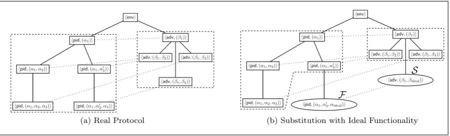
Figure 9: Substitution operation and the construction for the universal composability theorem – a sub-protocol is substituted for an ideal functionalityF and its sub-adversary by the simulatorS used in the universal composability proof
An ideal functionality is a protocol, i.e., every party contains a copy of the ideal functionality in its protocol tree, and all of these copies share a common state (see Section 3.1.7). Since such a copy of the ideal functionality is part of the protocol tree, we allow the basenames of each machine to require ideal or real protocol code, instead of classifying ideal machines by their party IDs, as in GNUC [28].
In contrast to previous work, we furthermore allow ideal functionalities to have children. Whenever ideal machines use common routines, such as communication channels, it is very convenient to be able to formalize such a routine as a child, e.g., as an ideal functionality for communication channels.
We adopt the restriction from GNUC that ideal machines can only communicate with ideal peers in the network and that ideal machines cannot be compromised.
Previous work [12, 28, 39] models ideal functionalities as a single, separate machine that has a direct connection to the rest of the protocol via a so-called dummy nodes that solely forwards messages between the ideal functionality and the parent protocol.
In a time-sensitive setting, however, an ideal functionality has to abstract several machines, each of which has their own timer. It is therefore much more natural to consider distributed ideal functionalities than having a central ideal functionality: in the centralized setting the ideal functionality would have to manage the timers of each machine it replaced (each of which was in different parties in the network), as well as manage the additional delay the dummy nodes create. In the distributed setting, on the other hand, each instance of the ideal functionality is a separate machine with its own timer, allowing for a much simpler construction.
In the following, we therefore use distributed ideal functionalities, in particular for our abstraction of the onion routing protocol used in Tor (see Section 6).
3.4.1 Central vs. Distributed Ideal Functionalities
Acentral ideal functionalityis a machine without parents that is a peer of so-calleddummy nodes. Similar to previous work, a dummy node is linked to a central ideal functionalityF(see below). Upon receiving a messages from its parent node, a dummy node forwards this message to the machineF. Analogously, upon receiving a message from the machine F, the dummy node forwards this message to its parent node. A dummy node can not have any children. Similar to functionality nodes, dummy node can not be compromised.
For the sake of convenience, we treat dummy nodes as re-wirings, i.e., reroutings. Formally, dummy nodes live at all points in time at once, we say they areomni-time machines. Upon receiving a message at timet they also forward the message at time t, without any delay. It would be possible use normal machines as dummy nodes, but then the central ideal functionalities would have to compensate the time the dummy nodes need for forwarding messages.
In contrast to a central ideal functionality, we call an ideal functionality as considered in our frame-work, i.e., that consists of several nodes with the same code and a shared memory, a distributed ideal functionality.
![Figure 10: Boxed Protocol [Π]F and Multi-Session Functionality Fˆ](https://thumb-us.123doks.com/thumbv2/123dok_us/7899919.1311359/26.595.73.525.71.308/figure-boxed-protocol-p-multi-session-functionality-f.webp)