High-order Graph-based Neural Dependency Parsing
Zhisong Zhang1,2and Hai Zhao1,2,∗ †
1Center for Brain-Like Computing and Machine Intelligence,
Department of Computer Science and Engineering, Shanghai Jiao Tong University, Shanghai, 200240, China
2Key Laboratory of Shanghai Education Commission for Intelligent Interaction
and Cognitive Engineering, Shanghai Jiao Tong University, Shanghai, 200240, China
[email protected], [email protected]
Abstract
In this work, we present a novel way of using neural network for graph-based dependency parsing, which fits the neural network into a simple probabilistic model and can be further-more generalized to high-order parsing. In-stead of the sparse features used in traditional methods, we utilize distributed dense feature representations for neural network, which give better feature representations. The proposed parsers are evaluated on English and Chinese Penn Treebanks. Compared to existing work, our parsers give competitive performance with much more efficient inference.
1 Introduction
There have been two classes of typical approaches for dependency parsing: transition-based parsing and graph-based parsing. The former parses sen-tences by making a series of shift-reduce decisions (Yamada and Matsumoto, 2003; Nivre, 2003), while the latter searches for a tree through graph algo-rithms by decomposing trees into factors. This paper will focus on graph-based methods, which are based
∗
Correspondence author.
†
This work was partially supported by the National Nat-ural Science Foundation of China (No. 61170114, and No. 61272248), the National Basic Research Program of China (No. 2013CB329401), the Science and Technology Commis-sion of Shanghai Municipality (No. 13511500200), the Eu-ropean Union Seventh Framework Program (No. 247619), the Cai Yuanpei Program (CSC fund 201304490199 and 201304490171), and the art and science interdiscipline funds of Shanghai Jiao Tong University, No. 14X190040031, and the Key Project of National Society Science Foundation of China, No. 15-ZDA041.
on dynamic programming strategies (Eisner, 1996; McDonald et al., 2005; McDonald and Pereira, 2006). In this recent decade, extensions have been made to use high-order factors (Carreras, 2007; Koo and Collins, 2010) in graph models and the high-est one considers fourth-order (Ma and Zhao, 2012). However, all those methods usually use sparse indi-cator features as inputs and linear models to get the scores for later inference process. They are easy to suffer from the problem of sparsity, and linear mod-els can be insufficient to effectively integrate all the sparse features in spite of various rich context that can be potentially exploited.
Distributed representations and neural network provide a way to alleviate such a drawback (Bengio et al., 2003; Collobert et al., 2011). Instead of high-dimensional sparse indicator feature vectors, dis-tributed representations use low-dimensional dense vectors (also known as embeddings) to represent the features, and then they are usually used in a neu-ral network. For example, in the traditional meth-ods, a word is usually expressed by a one-hot vector; while distributed representations use a dense vector. By appropriate representation learning (usually by back-propagations in neural network), these embed-dings can replace traditional sparse features and per-form quite well together with neural network.
In recent years, using distributed representations and neural network has gradually gained popularity in natural language processing (NLP) since the pio-neer work of (Bengio et al., 2003). Several neural network language models have reported exciting re-sults for the tasks of machine translation and speech recognition (Schwenk, 2007; Mikolov et al., 2010;
114
Wang et al., 2013; Wang et al., 2014; Wang et al., 2015). Many other tasks of NLP have also been re-considered using neural network, the SENNA sys-tem1(Collobert et al., 2011) solved the tasks of part-of-speech (POS) tagging, chunking, named entity recognition and semantic role labeling.
In this work, we utilize neural network for first-order, second-order and third-order graph-based de-pendency parsing, with the help of the existing graph-based parsing algorithms. For high-order parsing, it is performed after the first-order parser prunes unlikely parts of the parsing tree. We use neural network to learn dense representations for word, POS and distance information, and predict how likely the dependency relationships are for a sub-tree factor in the dependency tree. For unlabeled projective dependency parsing, we have put a free distribution of our implementation on the Internet2.
The remainder of the paper is organized as fol-lows: Section 2 discusses related work, Section 3 gives the background for graph-based dependency parsing, Section 4 describes our neural network model and how we utilize it with graph-based pars-ing and Section 5 presents our experiments, results and some discussions. We summarize this paper in Section 6.
2 Related Work
There has been a few of attempts to parse with neural network. For dependency parsing, (Chen and Manning, 2014) uses neural network for greedy transition-based dependency parsing. We explore graph-based methods in this work, which might be difficultly utilized with neural network. (Le and Zuidema, 2014) implements a generative depen-dency model with a recursive neural network, but the model is used for re-ranking which needsk-best candidates.
For constituency parsing, (Collobert, 2011) uses a convolutional neural network and solves the prob-lem with a hierarchical tagging process. (Socher et al., 2010) and (Socher et al., 2013) use recur-sive neural network to model phrase-based parse trees, but their methods might be unlikely general-ized to dependency parsing because a dependency
1
http://ronan.collobert.com/senna/
2
https://github.com/zzsfornlp/nngdparser
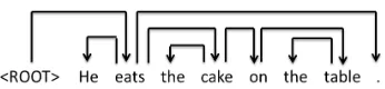
Figure 1: An example dependency tree.
parse tree has no non-terminal nodes while con-stituency parse trees are derived from the phrases structure.
Semi-supervised methods usually incorporate word representations as the embeddings for words in the projection layer in neural network; they usually make use of lots of unlabeled data to find the pat-terns in natural languages. If we utilize pre-trained word vectors (see in Section 5.1), our models can be regarded as semi-supervised to some extent. (Koo et al., 2008) uses Brown clustering algorithm to ob-tain word representations, but then transforms them into sparse features as additional features and again uses the traditional methods; while in neural net-work models including this net-work, the embeddings directly replace sparse features for inputs.
3 Graph-based Dependency Parsing 3.1 Background of Dependency Parsing
Syntax information is important for many other tasks (Zhang and Zhao, 2013; Chen et al., 2015). As a classic syntactic problem, dependency pars-ing aims to predict a dependency tree, which di-rectly represents head-modifier relationships be-tween words in a sentence. Figure 1 shows a de-pendency tree, in which all the links connect head-modifier pairs. By enforcing that all the nodes must have one and only one parent and the result-ing graphs should be acyclic and connected, we can get a directed dependency tree for a sentence (we usually add a dummy nodehrooti for the sentence as the highest level node).
pro-Figure 2: The decompositions of factors.
jective. Therefore this work also considers projec-tive dependency parsing only.
3.2 Graph-based Methods and their Decompositions
In graph-based methods, dependency trees are de-composed into specific factors that do not influence with each other. Each factor, usually represented by a sub-tree, is given a score individually based on its features. The score for a whole dependency treeT
is the summation of the scores of all the factors:
Scoretree(T) =
X
p∈f actors(T)
Scoref actor(p)
According to the sub-tree size of the factors, we can define the order of the graph model, some of the decomposition methods are shown in Figure 2. As the simplest case, the first-order model just con-siders sub-tree factor of single edge and its score is obtained by adding all the scores of the edges. For second-order models, another node is added into the factor, which can be either sibling or grandpar-ent. For third-order models, the simplest form is the grand-sibling decomposition, which adds both sibling and grandparent nodes. Existing work also applied various decompositions, such as third-order tri-sibling (Koo and Collins, 2010) which considers two siblings of the modifier and fourth-order tri-sibling (Ma and Zhao, 2012) which adds a grand-parent node on tri-siblings.
For the sake of simplicity and the convenient use of neural network, we only consider four models dis-cussed above (the sub-tree patterns of their factors are also shown in Figure 2). The notations for the four models are defined as follows:
• o1, first-order model
• o2sib, second-order model with sibling nodes • o2g, second-order model with grandparent nodes • o3g, third-order model with both sibling and
grand-parent nodes
3.3 Parsing Algorithms
Graph-based methods usually need to use dynamic programming based parsing algorithms, which make use of the scores of sub-trees for larger sub-trees in a bottom-up way. These algorithms solve the inference problem, that is, how to get an optimal tree given the scores for the parts. Our proposed parsers also take these algorithms as backbones and use them for inference.
In the traditional methods, scores are usually ob-tained directly from a linear model. In the learn-ing phase, parameter estimation methods for struc-tured linear models may adopt averaged perceptron (Collins, 2002; Collins and Roark, 2004) and max-margin methods (Taskar et al., 2004).
Still using all the existing parsing algorithms, this work focuses on improving scoring for the factors. In detail, our work uses neural network to deter-mine the scores. Nevertheless the traditional meth-ods might be difficultly extended to neural network because of the non-linearity. Therefore, we do not directly obtain scores from neural network. Instead we utilize a probabilistic model and obtain scores by some transformations, and then use these exist-ing parsexist-ing algorithms for inference.
4 Neural Network Parsers 4.1 The Probabilistic Model
For graph-based dependency parsing, it is not straightforward to extend the linear models to the more powerful nonlinear neural network, because we need to figure out the scores for the factors of the tree, which are not specified in the original tree-bank. That is, we only know which factors are in the correct parsing tree, but there are no natural ways to indicate how they are scored; the only intuition is to give high scores to the right factors and low scores to the wrong ones.
of words and tags and its formula is given as follows:
P r(words, tags, links)
=P r(words, tags)·P r(links present or not|words, tags)
≈P r(words, tags)· Y
1≤h,m≤n
P r(Lhm|tword(h), tword(m))
Unlike the original model, we determine only the probability for the parsing tree (the existence of the links):
P r(T|S) = Y
0≤h≤length(S) 0<m≤length(S)
P r(Lhm|context(h, m))
HereLhmis a binary variable with Bernoulli
distri-bution which means whether nodeh is the head of nodemandcontext(h, m)means the context of the two nodes which includes words, POS tags and dis-tance.
When looking for the best tree, we simply find the tree with highest probability (we use logarithmic form for more convenient computations). Consider-ing the sConsider-ingle-headed constrain for dependency tree construction, if we assign1toLHm, which makesH
the parent ofm, we must assign0to all otherLhm,
hmeans all the nodes that are not equal toH. The logarithmic probability can be rewritten as follows:
log(P r(T|S)) = X
0<m≤length(S)
log P r(LHm= 1)
+ X
0≤h≤length(S)
h6=H,h6=m
log P r(Lhm= 0)
HereH represents the real parent node of nodem. The formula is in the form of summation of the fac-tor scores, which are defined as:
Score(H, m) = log P r(LHm= 1)
+ X
0≤h≤length(S)
h6=H,h6=m
log P r(Lhm= 0)
After defining the score of each dependency fac-tor, we can apply the scores to the existing parsing algorithms (Eisner, 1996; McDonald et al., 2005).
4.2 High-Order Parsing
We now generalize the model to high-order parsing. In the first-order model, we define probabilities for
the head-modifier pair, which is the factor for first-order parsing. Naturally, we can define probabilities for high-order factors. The probability of a parse tree is the product of all its factors (either existing ones or wrong ones), the probability for one factor is again a binary value which means whether the factor exists in the dependency tree.
Using single-headed constraint again, for all the factors with the same node as the children, only one can exist in a legal parsing tree. The similar trans-formations can be performed and then again we will take the transformed scores as inputs to the corre-sponding parsing algorithms.
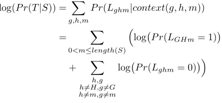
We describe the high-order extension by taking theo2gmodel as an example and other models can be handled in a similar way. We will use the simi-lar notations: Lghm is the binary variable that
indi-cates the factor with nodegas grandparent, node h
as head and nodemas modifier exists in the parse tree. We continuously useHas the parent ofmand
Gas its grandparent so thatLGHmis1(representing
an existing factor) in the parser tree. The logarithmic probability can be given by the following equation:
log(P r(T|S)) = X
g,h,m
P r(Lghm|context(g, h, m))
= X
0<m≤length(S)
log P r(LGHm= 1)
+ X
h,g h6=H,g6=G h6=m,g6=m
log P r(Lghm= 0)
4.3 Neural Network Model
Now we adopt feed-forward neural network to learn and compute the probability for a factor. The inputs for the network are features for a factor such as word forms, POS tags and distance, and the output will be the probability that the factor exists in the parse tree. Figure 3 shows the structure of our neural network for the o2g model, the networks for other models will be similar.
in-Figure 3: The structure of neural network foro2gmodel for an example input factor “cake→on→table”. Here we only demonstrate the case of a three-word window.
cludes the embeddings for features, where dis the dimension for the embedding,N is total number of possible features.
For the rest of the network, it can be viewed as a fully-connected feed-forward neural network with two hidden layers and a probabilistic output layer (we use a two-way softmax output unit to compute the probability). For the hidden layers, we use hy-perbolic tangent as activation function.
The training objective is to maximize the log-arithmic probability of parse trees with an L2-regularization term to avoid over-fitting, which equals to minimizing the cross-entropy loss with L2-regularization:
L(θ) =−X S
log P r(T|S)
+λ 2 · kθk
2
Hereθmeans parameters of the neural network and
λis the hyper-parameter for weight decay. We ini-tialize all the weights with random values and use mini-batch stochastic gradient descent for training.
4.4 Feature Sets
We utilize three kinds of features:
• Word forms (inside a specified sized window) • POS tags (for each word)
• Distance (to the node’s parent in the factor)
Using embeddings and neural network, we only need to provide unigram features, which will be mapped to embeddings in the neural network. The connections between features will be exploited by the non-linear computations of the neural network. Those three kinds of features are treated in the
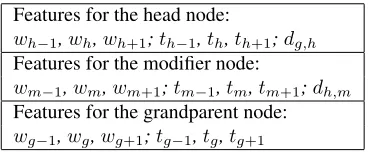
Features for the head node:
wh−1,wh,wh+1;th−1,th,th+1;dg,h Features for the modifier node:
wm−1,wm,wm+1;tm−1,tm,tm+1;dh,m Features for the grandparent node: wg−1,wg,wg+1;tg−1,tg,tg+1
Table 1: Features for the o2g model (with three-word windows).w: words,t: POS tags,d: distance. +1 and -1 means neighboring indexes.
same way as strings in the vocabulary, and special prefix strings are added to POS and distance fea-tures to differ them from word feafea-tures (“POS ” and “ distance ” respectively).
Again, take the situation foro2gmodel as an ex-ample, there are three nodes in a factor:gfor grand-parent, h for head and m for modifier. We show the features in Table 1 when considering three-word window, there will be three word forms and three tags for each node,handmboth have one distance feature whilegdoes not have one because its parent is unknown at this time. In fact, larger-sized context can be included and a seven-word window is actu-ally considered for later experiments.
4.5 Integrating Lower-order Models for Higher-order Parsing
two lower-order scores are integrated. Specifically, the score for the factor(g, h, s, m)will include the lower-order scores of o1 and o2sib in addition to the third-order scoreo3gScore(g, h, s, m)fromo3g
model. The integration of the scores can be shown by the following equation:
Score(g, h, s, m) = o1Score(h, m)
+ o2sibScore(h, s, m)
+ o3gScore(g, h, s, m)
More importantly, we may let the first-order model to serve as an edge-filter for high-order pars-ing. This type of pruning has been used by many graph-based models (Koo and Collins, 2010; Rush and Petrov, 2012) to avoid too expensive operations in high-order parsing. For our model, we utilize our own first-order neural network model which will produce the probabilities for all the edges in the graph. We simply set a pruning threshold so that all edges whose probabilities are under the thresh-old will be discarded for high-order parsing.
4.6 Efficient Neural Network Computation
This subsection introduces two techniques to speed up neural network computation.
Efficient computation strategies have been ex-plored extensively for neural network language models (Morin and Bengio, 2005; Mnih and Hinton, 2008; Vaswani et al., 2013). These models consider speeding up the output softmax layer which contains thousands of neurons. However, it is not the case for our neural network as the output layer of our net-work only has two neurons. Main computation cost in our network is from the first hidden layer, which needs matrix multiplications and the hyperbolic tan-gent activation calculations for the hidden neurons.
Similar to some previous work (Devlin et al., 2014; Chen and Manning, 2014), we apply the pre-calculation strategy to speed up the most concerned computation. This can be implemented as calculat-ing a lookup table for the first hidden layer (val-ues before computing activation function), which can replace the operations of the looking-up for em-bedding layer and the matrix multiplication for sec-ond layer (first hidden layer after). With the pre-calculation table, we only need to look up the
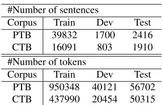
corre-#Number of sentences
Corpus Train Dev Test
PTB 39832 1700 2416
CTB 16091 803 1910
#Number of tokens
Corpus Train Dev Test
PTB 950348 40121 56702
CTB 437990 20454 50315
Table 2: Statistics for the data sets for dependency pars-ing.
sponding matrix multiplication results for each posi-tion’s input and add them together to get the values for the first hidden layer.
Another technique is to pre-calculate a hyperbolic tangent table, which will replace the computation for the activation function with a table looking-up pro-cess.
5 Experiments and Discussions
The proposed parsers are evaluated on English Penn Treebank (PTB3.0) and Chinese Penn Tree-bank(CTB7.0). For all the results, we report unla-beled attachment scores (UAS) excluding punctua-tions3as in previous work (Koo and Collins, 2010; Zhang and Clark, 2008). In Table 2, we show statis-tics of both treebanks.
For English, we follow the splitting conventions, using sections 2-21 for training, 22 for developing and 23 for test. We patch the Treebank using Vadas’ NP bracketing4 (Vadas and Curran, 2007) and use the LTH Converter5(Johansson and Nugues, 2007) to get the dependency treebank. We use Stanford POS tagger (Toutanova et al., 2003) to get predicted POS tags for development and test sets, and the ac-curacies for their tags are 97.2% and 97.4%, respec-tively.
For Chinese, we follow the convention described in (Zhang and Clark, 2008). The dependencies are converted with Penn2Malt tool6. As in previous work, we use gold segmentation and POS tags.
For both treebanks, all the graph-based parsers
3
Punctuations are the tokens whose gold POS tag is one of
{“ ” : , .}for PTB andP Ufor CTB.
4http://sydney.edu.au/engineering/it/∼dvadas1 5
http://nlp.cs.lth.se/software/treebank converter
6
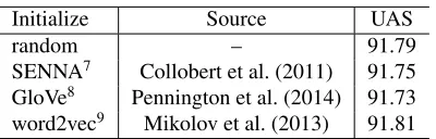
Initialize Source UAS
random – 91.79
SENNA7 Collobert et al. (2011) 91.75
GloVe8 Pennington et al. (2014) 91.73
word2vec9 Mikolov et al. (2013) 91.81
Table 3: Accuracies for different initializations, with first-order models on dev set.
run on the same machine with Intel Xeon 3.47GHz CPU using single core.
5.1 Different Embedding Initializations
We initialize the embedding matrix (only the parts for the embeddings of words) with some trained word embeddings or word vectors as shown in Table 3. Compared to the random initialization method, using pre-trained embeddings does not bring too sig-nificant improvements. We contribute this mostly to already large enough training set. In fact, the num-ber of the training samples fed to the network is over 20 million. Another possible reason is that the em-bedding initialization only works for word form fea-tures and other feafea-tures such as POS tags and dis-tance will have to be initialized with random val-ues. Those two types of initializations existing in the same space may cause possible inconsistence. Based on the above empirical results and compari-son, we will only use random initialization for our parsers.
5.2 Pruning
For high-order models, their full training can be computationally expensive or even impossible, so we must prune unlikely dependencies as we stated before in Section 4.5. We use a simple strategy by setting a fixed probability threshold and the results of different thresholds are shown in Table 4. In this table, the notations are defined as the following:
• Wt= %edges wrongly pruned in training set
• Wd= %edges wrongly pruned in dev set • #inst= number of instances for one iteration • Time= time for one iteration
• Acc.= UAS on dev set
With a large threshold, we might prune some cor-rect dependencies, but if the threshold is set smaller, more incorrect dependencies will remain and the
Threshold Wt Wd #inst(M) Time(min.)Acc.
0.01 0.47 1.41 315 29 92.41
0.001 0.13 0.58 764 65 92.47
0.0001 0.02 0.13 2591 220 92.43
Table 4: Effects of pruning methods with different thresh-olds (on English dev set with theo2sibmodel).
training will be more expensive. Even though those wrongly pruned dependencies are allowed, their scores are also too low to influence the inference. A threshold of 0.001 is finally chosen for other ex-periments in this work.
5.3 Main Results
As for detailed neural network setting, we use em-beddings of 50 dimensions, and the size of the two hidden layers are 200 and 40, respectively. We ini-tialize the learning rate as 0.1. After each iteration, the parser is tested on the development set and if the accuracy decreases, the learning rate will be halved. We train the models for 10 iterations and select the ones that perform best on the development set.
For the inputs, we consider a seven-word win-dow. Notice that only with distributed represen-tations, can we incorporate such very-long-context features. We ignore the words that occur less than 3 times in the training treebank and use a default token to represent unknown words.
Our evaluations will follow the setting in (Chen and Manning, 2014), which reported results of the transition-based neural network parser. For graph-based parsers, in order to get exact comparisons be-tween traditional methods and neural network meth-ods, we run the traditional graph-based parsers un-der the same executing environment as our parsers. In detail, MSTParser10foro1 ando2sibmodels and MaxParser11 (Ma and Zhao, 2012) foro2gando3g
models are respectively used for comparison. Notice that in recent years, there have been plenty of graph-based parsers which utilize various techniques and obtain state-of-art results (Rush and Petrov, 2012; Zhang and McDonald, 2012), however, they will not be included in the comparisons for the reason that we only concern about basic graph-based parsing
al-10
http://sourceforge.net/projects/mstparser/
11http://sourceforge.net/projects/maxparser/, this is a C++
Parser UAS Root CM Speed o1-nn 91.77 96.61 35.89 150 o2sib-nn 92.35 96.40 39.86 109 o2g-nn 92.18 96.85 38.45 89 o3g-nn 92.52 96.81 41.10 38 o1-M st 91.31 95.12 36.67 18 o2sib-M st 91.99 95.90 39.74 14 o2g-M ax 92.12 96.03 40.11 2 o3g-M ax 92.60 96.31 42.63 0.3
transition 92.0 – – 1013
Table 5: Results on PTB, the English treebank.
Parser UAS Root CM Speed
o1-nn 83.59 76.86 26.60 112 o2sib-nn 86.00 77.59 31.94 70 o2g-nn 84.13 77.75 27.59 49 o3g-nn 86.01 78.06 31.88 11 o1-M st 83.31 71.57 27.49 9 o2sib-M st 85.34 75.60 32.98 8 o2g-M ax 84.96 76.32 31.94 1 o3g-M ax 86.41 78.22 34.82 0.1
transition 83.9 – – 936
Table 6: Results on CTB, the Chinese treebank.
gorithms.
We report three accuracy metrics, UAS, Root (percentage of the root words correctly identified), CM (complete rate, percentage of sentences for which the whole tree is correct) and Speed (num-ber of sentences per second). For Chinese, the UAS and CM both consider root words.
Tables 5 and 6 show the results for PTB and CTB. As for name suffix in the tables,nnmeans our neu-ral network graph-based parsers, M st means Mst-Parser, M axmeans MaxParser, transitionmeans the transition-based neural network parser (Chen and Manning, 2014).
From the results, we can see that our parsers can get similar or even better results compared to the traditional graph-based models of the correspond-ing orders. In addition, our speed is faster (notice that even our o3g parser is faster than the tradi-tional first-order graph-based parser). Compared to the transition-based neural network parser, although our parsers are not that fast (transition-based parsers usually have O(n) time complexity), they give better performance in accuracies.
5.4 Discussions
We find that integrating lower-order models into high-order parsing leads to better results. Although the high-order factors already include the lower-order parts, it might be hard for the neural network to decide whether the whole factor is correct. Dur-ing trainDur-ing, we specify a factor as a positive sample only if all the dependencies in it are correct because we only do a binary classification. This might be the limitation for our high-order model and might ex-plain the reason why some of our high-order parsers do not surpass traditional ones in accuracy, we might need more appropriate object functions to improve its learning.
Compared to the features of traditional methods, the only information beyond the proposed feature set is the words that fall out of the windows between the nodes in the factor (previously called in-between features) because so far we only use fixed-size inputs for the feed-forward neural network. Extra opera-tions for embedding vectors (like adding embedding vectors) and other forms of neural networks (such as convolutional neural network which can consider the context of a whole sentence) might be explored in the future.
6 Conclusions
In this paper, we show a way to use neural network for graph-based dependency parsing and the method is also suitable for high-order parsing. We show that using distributed representations for neural net-work to replace traditional sparse features in tradi-tional graph models can be suitable for dependency parsing, even though only using a feed-forward net-work. From the evaluation results and comparison with existing models, we show that the proposed parsers get good results with quite efficient infer-ence even though graph-based models usually need at least cubic-time for inference.
References
Yoshua Bengio, R´ejean Ducharme, Pascal Vincent, and Christian Janvin. 2003. A neural probabilistic lan-guage model. Journal of Machine Learning Research (JMLR), 3:1137–1155, March.
guistics: Human Language Technologies, pages 498– 507, Montr´eal, Canada, June. Association for Compu-tational Linguistics.
Holger Schwenk. 2007. Continuous space language models. Computer Speech and Language, 21(3):492– 518.
Richard Socher, Christopher D. Manning, and Andrew Y. Ng. 2010. Learning continuous phrase representa-tions and syntactic parsing with recursive neural net-works. InProceedings of the NIPS-2010 Deep Learn-ing and Unsupervised Feature LearnLearn-ing Workshop. Richard Socher, John Bauer, Christopher D. Manning,
and Ng Andrew Y. 2013. Parsing with compositional vector grammars. InProceedings of the 51st Annual Meeting of the Association for Computational Linguis-tics (Volume 1: Long Papers), pages 455–465, Sofia, Bulgaria, August. Association for Computational Lin-guistics.
Ben Taskar, Dan Klein, Mike Collins, Daphne Koller, and Christopher Manning. 2004. Max-margin parsing. In Dekang Lin and Dekai Wu, editors, Proceedings of EMNLP 2004, pages 1–8, Barcelona, Spain, July. As-sociation for Computational Linguistics.
Kristina Toutanova, Dan Klein, Christopher D. Manning, and Yoram Singer. 2003. Feature-rich part-of-speech tagging with a cyclic dependency network. In PRO-CEEDINGS OF HLT-NAACL, pages 252–259. David Vadas and James Curran. 2007. Adding noun
phrase structure to the penn treebank. In Proceed-ings of the 45th Annual Meeting of the Association of Computational Linguistics, pages 240–247, Prague, Czech Republic, June. Association for Computational Linguistics.
Ashish Vaswani, Yinggong Zhao, Victoria Fossum, and David Chiang. 2013. Decoding with large-scale neu-ral language models improves translation. In Pro-ceedings of EMNLP-2013, pages 1387–1392, Seattle, Washington, USA, October. Association for Computa-tional Linguistics.
Rui Wang, Masao Utiyama, Isao Goto, Eiichro Sumita, Hai Zhao, and Bao-Liang Lu. 2013. Converting continuous-space language models into n-gram lan-guage models for statistical machine translation. In Proceedings of the 2013 Conference on Empirical Methods in Natural Language Processing, pages 845– 850, Seattle, Washington, USA, October. Association for Computational Linguistics.
Rui Wang, Hai Zhao, Bao-Liang Lu, Masao Utiyama, and Eiichiro Sumita. 2014. Neural network based bilin-gual language model growing for statistical machine translation. In Proceedings of the 2014 Conference on Empirical Methods in Natural Language Process-ing (EMNLP), pages 189–195, Doha, Qatar, October. Association for Computational Linguistics.
Rui Wang, Hai Zhao, Bao-Liang Lu, Masao Utiyama, and Eiichiro Sumita. 2015. Bilingual continuous-space language model growing for statistical machine trans-lation. IEEE/ACM Transactions on Audio, Speech, and Languange Processing, 23:1209–1220.
Hiroyasu Yamada and Yuji Matsumoto. 2003. Statisti-cal dependency analysis with support vector machines. In Proceedings of the 8th International Workshop on Parsing Technologies (IWPT), pages 195–206, April. Yue Zhang and Stephen Clark. 2008. A tale of two
parsers: Investigating and combining graph-based and transition-based dependency parsing. InProceedings of the 2008 Conference on Empirical Methods in Nat-ural Language Processing, pages 562–571, Honolulu, Hawaii, October. Association for Computational Lin-guistics.
Hao Zhang and Ryan McDonald. 2012. General-ized higher-order dependency parsing with cube prun-ing. In Proceedings of the 2012 Joint Conference on Empirical Methods in Natural Language Process-ing and Computational Natural Language LearnProcess-ing, pages 320–331, Jeju Island, Korea, July. Association for Computational Linguistics.