Proceedings of Recent Advances in Natural Language Processing, pages 723–732,
Unsupervised Learning of Morphology with Graph Sampling
Maciej Sumalvico University of Leipzig
NLP Group, Department of Computer Science Augustusplatz 10, 04109 Leipzig
sumalvico@informatik.uni-leipzig.de
Abstract
We introduce a language-independent, graph-based probabilistic model of mor-phology, which uses transformation rules operating on whole words instead of the traditional morphological segmentation. The morphological analysis of a set of words is expressed through a graph hav-ing words as vertices and structural rela-tionships between words as edges. We define a probability distribution over such graphs and develop a sampler based on the Metropolis-Hastings algorithm. The sampling is applied in order to deter-mine the strength of morphological rela-tionships between words, filter out acci-dental similarities and reduce the set of rules necessary to explain the data. The model is evaluated on the task of finding pairs of morphologically similar words, as well as generating new words. The results are compared to a state-of-the-art segmentation-based approach.
1 Introduction
The aim of unsupervised learning of morphology is to explain structural similarities between words of a language and discover mechanisms allowing one to predict or analyze unseen words using only a plain wordlist or an unannotated corpus as input. A vast majority of approaches to this problem con-centrates onmorphological segmentation, i.e. seg-mentation of words into minimal structural units, called morphs (Hammarstr¨om and Borin, 2011), usually employing statistical or machine learning methods.
While the segmentation approach has proven successful in some applications (especially com-pound splitting), it is known to suffer from
seri-ous limitations, like e.g. its intrinsic difficulty of handling non-concatenative morphology. Further-more, phenomena like morphophonological rules (reflected by the orthography), allomorphs, or in-teractions between morphemes, are especially dif-ficult to discover in an unsupervised setting, which is why most approaches limit themselves to rudi-mentary marking of postulated morpheme bound-aries in the word’s surface form. Because of the lack of morphotactical information, there is also no straightforward way to utilize such methods for generating new words: considering arbitrary mor-pheme sequences overgenerates massively and ad-ditional filtering approaches are needed, like the ones presented by (Rasooli et al.,2014). Finally, the notion of morpheme itself, although widely ac-cepted in linguistics, has also been subject to criti-cism (e.g.Aronoff,1976,2007;Anderson,1992). An alternative linguistic theory, called Whole Word Morphology (Ford et al.,1997;Singh et al., 2003) (henceforth WWM), seems in our opinion particularly useful from the point of view of un-supervised learning. In WWM, the structural reg-ularities between words are expressed as patterns operating simultaneously on multiple levels of lex-ical representation (phonologlex-ical, syntactic, se-mantic). For example, the structural relationship betweencatandcatswould be captured by the fol-lowing rule:1
"
PHON: /X/
SYNT: N,SG SEM: ♠
# ↔
"
PHON: /Xs/
SYNT: N,PL SEM: many♠
#
(1) The bidirectional arrow postulates, that if there is a word matching the pattern on one side of the rule, a counterpart matching the other side should also be a valid word. There is no notion of ‘in-ternal word structure’ and neither of the words is 1For the sake of simplicity, we discard the allophony in the phonological representation and present the semantic layer in an extremely schematic way.
said to be morphologically ‘more complex’ than the other. The variableX stands for an arbitrary sequence of phonemes, which is retained on both sides of the rule. While the particular represen-tations are further decomposable, for instance the phonological one in syllables and phonemes, the smallest unit of the language that combines all three layers is the word, and not the morpheme.
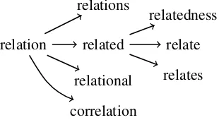
In this way, the morphological structure of a lexicon can be expressed as a graph, in which words constitute vertices and pairs of words fol-lowing a regular structural pattern are connected with an edge, labeled with the corresponding rule. For the task of unsupervised learning, we see it as an advantage to learn a relation operating directly on observable objects (i.e. words), rather than some vaguely defined and theory-dependent un-derlying representation, like morpheme segmen-tation.
In the remainder of this paper, we briefly review previous unsupervised approaches to morphology (Sec. 2), present a generative probabilistic model for graphs of word derivations (Sec. 3), along with inference algorithms suited for unsupervised learning (Sec.4). Our method is evaluated in Sec. 5.
2 Related Work
The approaches focusing on segmentation of words into smaller meaningful units have a long history, ranging from heuristic methods (Harris, 1955; Goldsmith, 2006) to the more recent ap-proaches employing complete probabilistic mod-els. A particularly successful example of the lat-ter is Morfessor (Creutz and Lagus, 2005; Vir-pioja et al., 2013). Further probabilistic models include probabilistic hierarchical clustering (Can, 2011) and log-linear models (Poon et al., 2009). The yearly competition MorphoChallenge ( Ku-rimo et al.,2010), which took place from 2005 un-til 2010, provides a good overview on the state of the art in morphological segmentation.
Another line of research concentrates on find-ing pairs of morphologically related words and us-ing them to discover more general patterns. Var-ious similarity measures are often used to iden-tify such pairs, including orthographic and context similarity, or a combination of both (Yarowsky and Wicentowski, 2000; Baroni et al., 2002; Kirschenbaum, 2013). The first approach explic-itly mentioning Whole Word Morphology as
lin-relation related relate relates relations
relational correlation
relatedness
Figure 1: An example tree of word derivations. Edge labels are omitted for better readability.
guistic foundation has been presented by ( Neu-vel and Fulop, 2002), followed by a graph clus-tering method (Janicki, 2013) and a graph-based probabilistic model (Janicki, 2015). Recently, also word embeddings have been used to in-duce word-based transformation rules (Soricut and Och, 2015;Narasimhan et al., 2015). The latter method also produces graph-based representations of morphology, but is eventually evaluated on the segmentation task.
While, to our best knowledge, sampling from a probability distribution over graph structures has not yet been applied in the task of learn-ing morphology, it has been successfully applied in other NLP tasks, notably unsupervised depen-dency parsing (Mareˇcek,2012;Teichmann,2014) and machine translation (Peng and Gildea,2014). 3 The Probabilistic Model
The model described here is a slight modification of the one introduced by (Janicki, 2015). Our goal is a probability distributionP r(V, E|R)over graphs (consisting of a set of verticesV and a set of labeled edgesE), given a set of transformation rules R. A single graph represents a hypothesis about the origin of words: the root nodes consti-tute the idiosyncratic part of the lexicon, i.e. they correspond to words, that are not derived from any other and must be memorized. Once some words are introduced, further ones can be derived using the transformation rules. Such derivations correspond to edges leading to new nodes. We restrict the allowed structure of the graphs to di-rected forests: they must not contain cycles and every node has at most one ingoing edge, i.e. ev-ery word has a unique analysis. Accordingly, we consider directed transformation rules.
probability of the rule set is then proportional to the product of probabilities of individual rules:
P r(R)∝ Y r∈R
π(r) (9)
The distribution P r(R) penalizes complex mod-els: it attributes lower probabilities to large rule sets and specific, sophisticated rules.
4 Inference
While (Janicki, 2015) used an optimization ap-proach to find the single best graph, our goal is to base the inference on large samples from the dis-tribution over graphs using a Markov Chain Monte Carlo sampler. In particular, we are going to be in-terested in expected values of certain functions of the graph with respect to the edge structure, which is a latent variable. Thus, for a given function h
(e.g. measuring the frequency of a rule or the like-lihood of the graph), we want to be able to approx-imate the expectations of the following form:
EE|V,Rh(V, E) =X
E
h(V, E)P r(E|V, R) (10)
4.1 Finding Candidate Rules
We begin by extracting all pairs of words that might be morphologically related from the given vocabulary. We follow the approach of (Janicki, 2015): we apply a modified FastSS algorithm ( Bo-cek et al.,2007) to find all pairs of words, that dif-fer with at most 5 characters at the beginning and at the end and with at most 3 characters within a single slot inside the word. Those numbers are configurable parameters, but we have found the above values to be sufficient to capture most mor-phological rules in many languages.
Each pair of words is used to extract a number of transformation rules of the form (cf. (1)):
/a1X1a2X2a3/→/b1X1b2X2b3/ (11)
whereX1, X2 are variable elements,a1, a3, b1, b3
are constants of at most 5 characters, anda2, b2are
constants of at most 3 characters.4 There are usu-ally many rules that can be derived from a single pair of words, depending on whether we assign the common substrings of both words to the variable elementsX1, X2, resulting in more general rules,
or to the constants, resulting in more specific rules. 4In casea
2andb2are both empty,X1andX2are merged
into a single variableX.
For example, three of many rules that can be ex-tracted from the pair hrelate,correlatei are given below:
/X/ → /corX/ /rX/ → /corrX/
/rXate/ → /corrXate/ (12) In order to reduce the number of candidate rules and edges to tractable sizes, we apply the follow-ing filterfollow-ing criteria:
max. number of rules: onlyNmaxmost frequent
rules are kept;
max. number of edges per word pair: only k
most general rules are extracted from each word pair;
min. rule frequency: only rules occurring in at leastnminword pairs are kept.
In all our experiments, we used fixed values of
Nmax = 10000, k = 5, nmin = 3, which led
to good results for training data of various sizes. Those values can thus be safely used as default setting, without the need of parameter tuning.
4.2 The Sampler
Having a set of rules R and a vocabulary V, we are ready to draw samples of edge sets from the distributionP r(E|V, R), which is proportional to
P r(V, E|R)up to a normalizing constant. In the following, we will define a sampler based on the Metropolis-Hastings algorithm, which belongs to a larger family of Markov Chain Monte Carlo methods.
The key idea of Markov Chain Monte Carlo methods is, given a probability distribution f, to construct a Markov chain, for whichf is the lim-iting distribution (Robert and Casella,2005). The Metropolis-Hastings algorithm (Metropolis et al., 1953;Hastings,1970) provides a relatively simple recipe for such chain. It involves an instrumental distributionq(y|x)used to propose the next itemy
of the sample given the current itemx. Then, the next item of the sample is taken to be eithery or
x, depending on whether the proposal is accepted or rejected. The probability of acceptance is:
α(x, y) = min
f(y)
f(x)
q(x|y)
q(y|x),1
computation only involves quotients of their val-ues. Also,qdoes not have to bear any relationship tof. It is sufficient that every point of the sample space, for whichfis nonzero, can be reached from any other in a finite number of steps usingq. Then (13) implies that the resulting Markov chain has
f as its limiting distribution. Although the sam-ple obtained from such chain is not independent, it can be used for approximating expectations like (10).
The preprocessing step described in the previ-ous section provides us with a set of all candidate edgesE, which can be created by the rules fromR. The idea for a proposal distributionq(·|E), given the current set of edges E, is the following: we choose an edgeeuniformly fromE. If it is already present inE, we delete it, if not, we add it. In this way, we obtain a proposal for the next set of edges
E0. Note that in this way we can reach any graph from any other in a finite number of steps by first deleting all the edges of the first graph and then adding all the edges of the second graph one by one.
There is however one problem with this ap-proach: while deleting an edge is always possible, adding one could result in an ill-formed graph (e.g. create a cycle). If we simply discarded such pro-posals and proposed staying with the current graph instead, such procedure would still yield a valid instrumental distribution and a valid MCMC sam-pler. While the resulting chain would still be the-oretically correct, its so-called mixing properties would be very bad, meaning that it would need an extremely large number of iterations to converge to the limiting distribution. For this reason, we are going to introduce additional moves which make adding of an edge possible in most cases.
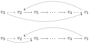
Let’s consider adding a new edgev1 →r v2. The
first problematic case is when the new edge would create a cycle, i.e. v1 is already a descendent of
v2. Letv3denote the parent ofv2,v5 the
immedi-ate child ofv2which leads tov1andv4the parent
ofv1(see Fig.2). We have two possibilities to add
an edge betweenv1 andv2 by ‘cutting out’ either
v1 orv2 from its place in the tree. Both variants
involve adding and deleting two edges. We refer to this kind of operation as ‘flip’. The variant to be used is chosen randomly each time a ‘flip’ move is to be applied. Note that a ‘flip’ move might be impossible if the other edge to be added (v3 →v1
or v3 → v5, respectively) is not available in E.
v3 v2 v5 . . . v4 v1
v3 v2 v5 . . . v4 v1
Figure 2: The two variants of the ‘flip’ operation. The deleted edges are dashed and the newly added edges dotted. The goal of the operation is to make possible adding an edge fromv1tov2without
cre-ating a cycle.
In this case, we propose staying with the current graph, which, as already mentioned, does not un-dermine the validity of the sampler. The absence of other involved edges (e.g. v3 → v2 in casev2
is a root) or the overlapping of some nodes (e.g.
v5=v1andv4 =v2ifv1is a child ofv2directly)
can be simply ignored as the move is still valid. Another problematic case arises when the newly added edge v1 →r v2 would not create a cycle,
butv2already has an ingoing edge (possibly even
fromv1, but with a different label). In this case,
we simply exchange the previous ingoing edge of
v2for the new one.
It is important to point out, that all moves are re-versible and that the resulting proposal distribution is symmetric. The move is uniquely determined by the choice of the edgeeto be added or deleted, except for the ‘flip’ case, where additionally one of the two variants of the move is randomly cho-sen. In case of adding or removing a single edge without side effects, selecting the same edge again reverses the operation. If the edge to be added is exchanged for another, selecting the previously deleted edge will reverse it. Finally, the first vari-ant of ‘flip’ on v1 → v2 can be reversed by the
second variant onv4 →v1and the second variant
onv1 →v2can be reversed by the first variant on
v2→v5.
Note, that the complexity of a single sampling iteration is onlyO(h), withhbeing the maximum height of a tree, sinceh operations are needed to determine whether v1 is a descendant of v2. In
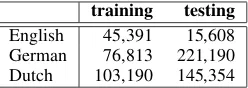
training testing English 45,391 15,608 German 76,813 221,190 Dutch 103,190 145,354
Table 1: The size (number of words) of datasets used for the analysis task.
the EM algorithm, which requires a space of real-valued vectors).
4.4 Model Fitting
Once the optimal model is selected, we can deter-mine optimal values for the parameter vectorΘR.
For this purpose, we use the Monte Carlo EM al-gorithm (Wei and Tanner,1990), which is a vari-ant of EM using a sampler to approximate the ex-pected values. In the maximization step, we set the
θrvalues to their maximum a-posteriori likelihood estimates:
θ(t+1)
r :=
EE|V,R,Θ(t)
R [nr] +α−1
mr+α+β−2 (19)
5 Evaluation
We evaluate our approach on the tasks of morpho-logicalanalysisandgeneration.
5.1 Analysis
As we intend to avoid postulating internal word structure, the task of analysis is defined as link-ing an unknown word to morphologically similar words from a known lexicon. We consider a pair of words to be morphologically similar if one word can be derived from the other using a single mor-phological operation (e.g. affix insertion, deletion or substitution). Pairs of morphologically similar words can also be extracted from segmentations by computing edit distance on morpheme sequences – words are considerered morphologically similar if such distance is equal to 1 and the difference does not include stems.
Dataset We use the CELEX lexical database to
derive training and evaluation data. CELEX pro-vides data for English, German and Dutch, includ-ing morphological segmentation, labelinclud-ing of in-flectional classes and corpus frequency. For train-ing, we use words with nonzero corpus frequency, while the remaining words, i.e. those with zero frequency, constitute the testing dataset. The size of the datasets is shown in Table1.
–MS +MS English 9,434 3,943 German 8,432 4,888 Dutch 9,026 4,743
Table 2: The model size (number of rules) before and after model selection.
Language Model Precision Recall F-score
English Morfessor–MS 74.4 %38.5 % 41.4 %73.2 % 53.2 %50.5 % +MS 53.8 % 69.3 % 60.6 % German Morfessor–MS 75.1 %56.4 % 38.8 %67.8 % 51.2 %61.6 % +MS 65.1 % 62.8 % 63.9 %
Dutch Morfessor–MS 73.1 %42.5 % 39.2 %68.1 % 51.0 %52.3 % +MS 54.1 % 63.1 % 58.3 % Table 3: Results for the analysis task.
Experiment setup We report the results for two
different setups: with model selection (+MS) and without it (–MS). We also compare our results to Morfessor Categories-MAP (Creutz and Lagus, 2005). In addition to morpheme segmentations, this tool labels each morpheme as prefix, affix or stem, which enables us to convert its output into morphologically similar pairs using the edit dis-tance method.6 The training dataset also consti-tutes the known lexicon, i.e. we evaluate pairs of similar words(w1, w2)withw1 coming from the
training andw2 from the testing dataset.
Results The results are shown in Table 3. The
setup with model selection achieves the best per-formance for all three languages, which demon-strates the usefulness of this step. The difference is especially clear for English, where the setup without model selection performs worse than Mor-fessor. Our method also manages to capture non-concatenative morphology: pairs like German (findet, f¨andet) or Dutch (televisiekanalen, tele-visiekanaal), are successfully detected. On the other hand, the method based on Morfessor seg-mentations suffers from low recall: even small er-rors in segmentation can result in a failure to dis-cover many similar pairs.
Table 2 shows another benefit of model selec-tion: reducing the number of rules approximately by half, which has a significant impact on the speeed of the analysis.
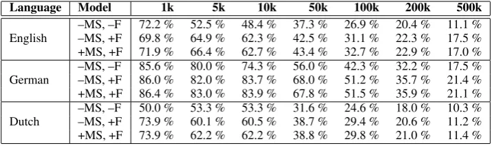
Language Model 1k 5k 10k 50k 100k 200k 500k
English –MS, –F–MS, +F 72.2 %69.8 % 52.5 %64.9 % 48.4 %62.3 % 37.3 %42.5 % 26.9 %31.1 % 22.3 %20.4 % 11.1 %17.5 % +MS, +F 71.9 % 66.4 % 62.7 % 43.4 % 32.7 % 22.9 % 17.0 % German –MS, –F–MS, +F 85.6 %86.0 % 80.0 %82.0 % 74.3 %83.7 % 56.0 %68.0 % 42.3 %51.2 % 35.7 %32.2 % 17.5 %21.4 % +MS, +F 86.4 % 83.0 % 83.9 % 67.8 % 51.5 % 35.9 % 21.1 %
Dutch –MS, –F–MS, +F 50.0 %73.9 % 53.3 %60.1 % 53.3 %60.5 % 31.6 %38.7 % 24.6 %29.4 % 20.6 %18.0 % 10.3 %11.2 % +MS, +F 73.9 % 62.2 % 62.2 % 38.8 % 29.8 % 21.0 % 11.4 %
Table 4: Results for the generation task. The scores show precision depending on the number of gener-ated words. (‘k’ means ‘thousand’).
5.2 Generation
In generation task, we evaluate the capability of the model to derive new, valid words using the learnt morphological rules. As the recall mea-sure for this task is hardly possible to compute (it would involve listing all and only words derivable from the training set), we evaluate the precision against the number of generated words.
Dataset For training, we use the same datasets
as in the analysis task (CELEX words with nonzero corpus frequency). The testing wordlists, which are supposed to contain at least all words obtainable from the training words within a single morphological operation, are built by merging the complete CELEX vocabulary with lists of Wik-tionary entries for the relevant language.
Experiment setup We conduct the experiment
on three different settings, depending on whether the model selection (MS) and the fitting (F) step are carried out or omitted.7 In case of omitting the fitting step, the rule probabilities (θr) are set according to (19), but using maximum rule fre-quency, i.e. the number of candidate edges in
E labeled with this rule, as nr. The generated words are ordered by their contribution to the log-likelihood of the data, which is equivalent to sort-ing accordsort-ing to the probability of the rule used to derived the word.
For this task, we do not include any compari-son to a segmentation-based approach. Such ap-proaches usually do not model morphotactics at all, or do it in a very simple way (like Morfes-sor Categories-MAP). Applying them to gener-ate new words leads to a disastrous overgenera-tion (e.g. every common morpheme can be re-peated many times), which renders a comparison 7The results for the +MS, –F case are omitted, because they are very similar to –MS, –F, and thus do not contribute anything noteworthy to the evaluation.
pointless. Segmentation models are simply not de-signed for the generation task.
Results The results shown in Table4 highlight
the importance of a proper fitting step, which in most cases improves the results considerably. On the other hand, the impact of the model selection step is rather insignificant. This is understandable: the goal of model selection is to eliminate weak, useless rules, while in the word generation task, the strongest rules are applied first.
6 Conclusion
References
Stephen R. Anderson. 1992. A-Morphous Morphology. Mark Aronoff. 1976. Word Formation in Generative
Grammar. MIT Press.
Mark Aronoff. 2007. In the Beginning was the Word.
Language83(4):803–830.
Marco Baroni, Johannes Matiasek, and Harald Trost. 2002. Unsupervised discovery of morphologically related words based on orthographic and semantic similarity. In Proceedings of the 6th Workshop of the ACL Special Interest Group on Phonology. vol-ume 6, pages 48–57.
Julian Besag. 2004. An introduction to Markov chain Monte Carlo methods. In Mark Johnson, Sanjeev P. Khudanpur, Mari Ostendorf, and Roni Rosenfeld, editors, Mathematical Foundations of Speech and Language Processing, Springer-Verlag New York, Inc., pages 247–270.
Thomas Bocek, Ela Hunt, and Burkhard Stiller. 2007. Fast Similarity Search in Large Dictionaries. Tech-nical report, University of Zurich.
Burcu Can. 2011. Statistical Models for Unsupervised Learning of Morphology and POS Tagging. Ph.D. thesis, University of York.
Mathias Creutz and Krista Lagus. 2005. Inducing the Morphological Lexicon of a Natural Language from Unannotated Text. In Proceedings of the International and Interdisciplinary Conference on Adaptive Knowledge Representation and Reasoning (AKRR’05).
Colin de la Higuera. 2010. Grammatical Inference: Learning Automata and Grammars. Cambridge University Press, New York, NY, USA.
Colin de la Higuera and Franck Thollard. 2000. Iden-tification in the Limit with Probability One of Stochastic Deterministic Finite Automata. InICGI ’00. pages 141–156.
Alan Ford, Rajendra Singh, and Gita Martohardjono. 1997. Pace P¯an.ini: Towards a word-based theory
of morphology. American University Studies. Series XIII, Linguistics, Vol. 34. Peter Lang Publishing, In-corporated.
John Goldsmith. 2006. An algorithm for the unsuper-vised learning of morphology. Natural Language Engineering12(1):353.
Harald Hammarstr¨om and Lars Borin. 2011. Unsuper-vised Learning of Morphology. Computational Lin-guistics37(2):309–350.
Zellig S Harris. 1955. From phoneme to morpheme.
Language31(2):190–222.
Wilfred K. Hastings. 1970. Monte Carlo Sampling Methods Using Markov Chains and Their Applica-tions. Biometrika57(1):97–109.
Maciej Janicki. 2013. Unsupervised Learning of A-Morphous Inflection with Graph Clustering. In Pro-ceedings of the Student Research Workshop associ-ated with RANLP 2013. pages 93–99.
Maciej Janicki. 2015. A Multi-purpose Bayesian Model for Word-Based Morphology. In Cer-stin Mahlow and Michael Piotrowski, editors, Sys-tems and Frameworks for Computational Morphol-ogy – Fourth International Workshop, SFCM 2015. Springer.
S. Kirkpatrick, C.D. Gelatt, and M. P. Vecchi. 1983. Optimization by Simulated Annealing. Science
220(4598):671–680.
Amit Kirschenbaum. 2013. Unsupervised Segmenta-tion for Different Types of Morphological Processes Using Multiple Sequence Alignment. In 1st In-ternational Conference on Statistical Language and Speech Processing, SLSP. Tarragona, Spain, pages 152–163.
Mikko Kurimo, Sami Virpioja, Ville Turunen, and Krista Lagus. 2010. Morpho Challenge 2005-2010: Evaluations and results. InProceedings of the 11th Meeting of the ACL-SIGMORPHON, ACL 2010. pages 87–95.
David Mareˇcek. 2012. Unsupervised Dependency Parsing. Ph.D. thesis, Charles University in Prague. Nicholas Metropolis, Arianna W. Rosenbluth, Mar-shall N. Rosenbluth, Augusta H. Teller, and Edward Teller. 1953. Equation of state calculations by fast computing machines. Journal of Chemical Physics
21(6):1087–1092.
Karthik Narasimhan, Regina Barzilay, and Tommi S. Jaakkola. 2015. An unsupervised method for un-covering morphological chains. TACL3:157–167. Sylvain Neuvel and Sean A. Fulop. 2002.
Unsuper-vised Learning of Morphology without Morphemes. In Proceedings of the 6th Workshop of the ACL Special Interest Group in Computational Phonology (SIGPHON). pages 31–40.
Xiaochang Peng and Daniel Gildea. 2014. Type-based MCMC for Sampling Tree Fragments from Forests.
Proceedings of the 2014 Conference on Empirical Methods in Natural Language Processing (EMNLP 2014)pages 1735–1745.
Hoifung Poon, Colin Cherry, and Kristina Toutanova. 2009. Unsupervised morphological segmentation with log-linear models. In Proceedings of Human Language Technologies The 2009 Annual Confer-ence of the North American Chapter of the Associ-ation for ComputAssoci-ational Linguistics on NAACL 09. page 209.
Christian P. Robert and George Casella. 2005. Monte Carlo Statistical Methods (Springer Texts in Statis-tics). Springer-Verlag New York, Inc., Secaucus, NJ, USA.
Rajendra Singh, Stanley Starosta, and Sylvain Neu-vel. 2003. Explorations in Seamless Morphology. SAGE Publications.
Radu Soricut and Franz Josef Och. 2015. Unsuper-vised Morphology Induction Using Word Embed-dings. InNAACL 2015. pages 1626–1636.
Christoph Teichmann. 2014. Markov Chain Monte Carlo Sampling for Dependency Trees. Ph.D. the-sis, University of Leipzig.
Sami Virpioja, Peter Smit, Stig-Arne Gr¨onroos, and Mikko Kurimo. 2013. Morfessor 2.0: Python Im-plementation and Extensions for Morfessor Base-line. Technical report, Aalto University, Helsinki. http://urn.fi/URN:ISBN:978-952-60-5501-5. Greg C. G. Wei and Martin A. Tanner. 1990. A
Monte Carlo Implementation of the EM Algo-rithm and the Poor Man’s Data Augmentation Al-gorithms. Journal of the American Statistical Asso-ciation85(411):699–704.