Proceedings of Recent Advances in Natural Language Processing, pages 103–110,
Fast and Accurate Decision Trees for Natural Language Processing Tasks
Tiberiu Boros*,**, Stefan Daniel Dumitrescu**and Sonia Pipa** *Adobe Experience Manager, Machine Learning, Adobe Systems **Research Institute for Artificial Intelligence, Romanian Academy
{boros}@adobe.com,{sdumitrescu,sonia}@racai.ro
Abstract
Decision trees have long been used in many machine-learning tasks; they have a clear structure that provides insight into the training data and are simple to con-ceptually understand and implement. We present an optimized tree-computation gorithm based on the original ID3 al-gorithm. We introduce a tree-pruning method that uses the development set to delete nodes from overfitted models, as well as a result-caching method for speed-up. Our algorithm is 1 to 3 orders of magnitude faster than a naive implementa-tion and yields accurate results on our test datasets.
1 Introduction
Decision trees (DTs) are a well-established classi-fication/prediction methodology in machine learn-ing, in which the model is (as the name suggests) a tree where each node is a decision and each leaf represents an output class (label/distribution). A node can have any number of children, but com-monly, most algorithms implement only binary trees with binary questions. Decision-tree clas-sifiers are a very popular choice, mainly because they are easy to train and, by analyzing the tree structure one can easily validate certain assump-tions or gain a better understanding of the cor-pora/task as opposed to, for example, neural net-works in which the model is a matrix of numbers offering no insight.
DTs have been widely used in natural and spo-ken language-processing tasks such as tagging (Schmid, 2013), named entity recognition (NER) (Szarvas et al.,2006), letter-to-sound (LTS) con-version (Pagel et al., 1998), text categorization (Lewis and Ringuette, 1994), parameter
estima-tion for statistical parametric speech synthesis (Zen et al.,2007).
One of the drawbacks of decision trees is their relatively modest performance in classification tasks. Current state-of-the-art approaches in nat-ural language processing and other research fields employ more powerful methodologies, such as Support Vector Machines (SVMs), Conditional Random Fields (CRFs), and complex neural net-work architectures.
In what follows, we propose an optimized deci-sion tree computation algorithm which follows the guidelines of the Iterative Dichotomiser 3 (ID3) algorithm (Quinlan,1986), but computes entropy and information gain using a single pass over the training data. We also address the issue of overfit-ting the training set by introducing a tree-pruning algorithm that tunes an already existing tree using a development set. For significant speed increase we implement a result-caching method. We show that tree-pruning achieves up-to-par accuracy on our datasets by comparing results obtained using (a) the unpruned version of the tree (b) the pruned version of the tree and (c) various state-of-the-art methods in identical training and testing condi-tions.
We argue that the training speed-boost ob-tained by using our computational enhance-ments, as well as the accuracy-boost obtained by tree-pruning make DTs a desirable choice for feature-engineering and for real-life applications, whenever speed of implementation/training with slightly lower results are acceptable.
2 Related Work
The simple and robust principle behind decision trees made them an ideal choice for both academic and industrial (applied) research. There are sev-eral papers that address construction and
tion principles applied, from which we selected those relevant to our approach. Su and Zhang
(2006) use independent information gain (IIG) to speed-up the process of tree construction and re-duce the complexity of the calculus, Dai and Ji
(2014) introduce an algorithm designed for dis-tributed computation of trees, based on mapre-duce. Quinlan (1987) introduces one of the first tree-pruning strategies, whileMehta et al.(1995) andRastogi and Shim(1998) use the a more prin-cipled approach, based on the Minimum Descrip-tion Length (MDL). Though MDL strategies work very well and are currently the main ingredient of statistical parametric speech synthesis (Zen et al.,
2009), for simple NLP tasks they add “overhead” and increase computational complexity at train-ing time. Other approaches to decision tree op-timization are aimed straight at tree-construction strategies and refer to randomization, bagging and boosting (Dietterich,2000).
Our proposed optimization methods (a) are based on the original ID3 algorithm with the
“missing-attribute” extension and (b) focus on discrete features (not continuous values).
3 Enhanced ID3 Computation
The Iterative Dichotomizer 3 (ID3) is an algorithm created by Ross Quinlan to generate a decision tree from a dataset. The computation starts with the entire datasetS at the root node. For each it-eration, the feature having the largest information gainIG(S)is located among the unused features. The setSis then split and the two children of the current node are created: one for the examples that contained the selected feature and second for those that did not. The algorithm continues recursively for each newly created node, until one of the stop conditions is encountered:
• A subset contains only examples belonging to the same class. In this case, the node is turned into leaf labeled with the name of the class.
• There is no unused feature to select, but the examples still do not belong to the same class. The node is also turned into a leaf, this time labeled with the most common class in the subset.
• We do not obtain any information gain when splitting by any unused feature. In this
situa-tion, the created leaf is also labeled with the most common class in current subset. The output of this algorithm will be a decision tree, with each non-terminal node representing the selected feature on which the data was split, and the terminal nodes (leafs) representing the class la-bel of the final subset of the branch.
3.1 Speed-Optimized Computation of Entropy and Information Gain
Before describing our proposed optimizations, we have to clarify our view of the algorithm’s data representation style. The standard way to view a dataset is that of a examples (instances) having a number of attributes and an output class. Each at-tribute (e.g. Temperature) can have several values (multinomial attribute, e.g. Hot, Average, Cold), an instance being a collection of a particular value for each of the available attributes. The ID3 im-plementation we propose handles missing features and treats attributes as a bag-of-words, meaning that an instance might have a feature like Tem-perature Hot, or TemTem-perature Cold. This allows greater flexibility, especially for NLP tasks, and is essentially similar to the classic data representa-tion style.
Returning to the ID3 algorithm training proce-dure, the decision to select a feature over another is given by the information gain. Given a datasetS withM features andN classes, information gain IGi(S)is the measure of the difference in entropy
in S after it was split on feature i, meaning we measure how much the uncertainty in S has de-creased by choosing to split byi. This implies run-ning overSfor each of theMfeatures to compute IGi(S)and selecting the maximum value.
Choos-ing to split by feature i will yield, two comple-mentary subsets ofS, one having all examples (in-stances) that have featurei, named theY esi
sub-set, the other having the remaining examples that do not have featurei(theNoi subset). Iteratively,
for each subset we have to find the next feature to split on, again running over all the examples in the subsets. We propose a way around these multi-ple passes over the dataset that brings a significant speed increase.
Starting from the definition, information gain is the difference in entropy of the initial set S and after the set was split on featurei(in allT subsets).
IGi(S) =H(S)−
X
t∈T
where H(S) is the entropy of the initial set S, H(t)the entropy of subsett, andP(t)is the frac-tion of elements intover the entire|S|. We note |S|as the number of instances inS.
H(S) =−XN
x=1
Px·log2Px (2)
wherePxis the number of instances of classx
divided by|S|.
The optimization we propose in this paper is based on creating a contingency matrix. By having a matrix that stores partial results and additional information, we are able to reduce the number of operations that are repeatedly executed in the clas-sical implementation of the ID3 algorithm.
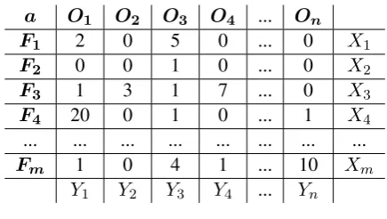
The proposed matrix is presented in Table 1, where O1,N notation is used for the N output
classes, and F1,M marks the M unique features.
Cells at index[i, j](from position[1,1]to[M, N]) keep the number of instances in the dataset that contain feature Fi of class Oj. To compute
H(S)andIGi(S)for every featurei, an iteration
through the dataset is required. To skip this step we add an extra row and column to the matrix: the M+1throw stores the total number of instances of
classOjand theN+1thcolumn stores the number
of instances that have labelFi.
Starting from the Entropy and Information Gain formulas, we developed the following set of equa-tions to compute these measures using the partial results stored in matrix.
a O1 O2 O3 O4 ... On
F1 2 0 5 0 ... 0 X1
F2 0 0 1 0 ... 0 X2
F3 1 3 1 7 ... 0 X3
F4 20 0 1 0 ... 1 X4 ... ... ... ... ... ... ... ...
Fm 1 0 4 1 ... 10 Xm
Y1 Y2 Y3 Y4 ... Yn
Table 1: Computation matrix
Now, the entropyH(S)can be written as:
H(S) =−
N
X
i=1
a[M+ 1, i]
|S| log2
a[M+ 1, i]
|S| (3) whereais our proposed contingency matrix and a[M + 1, i]refers to the last row that counts the number of instances having output classOi.
To calculate IGi(S), considering i as the
at-tribute to split on, we have to subtract fromH(S)
the entropy of the subsets multiplied by the proba-bility of splitting by featurei. The subsets, in our implementation, are always two: theY es subset containing all instances that have featureiand the Nosubset, with instances not containing featurei:
IGi(S) =H(S)−
[Pfeati·H(Y es) +Pfeati·H(No)] (4)
WherePfeati is:
Pfeati = a[i, N|S|+ 1] (5)
witha[i][N+ 1]being the number of instances that contain featurei, meaning the number of in-stances in theY essubset. ThePfeati is the
com-plement of Pfeati, meaning the number of
in-stances in theNosubset divided by the total num-ber of instances in|S|.
Moving on, the entropies of H(Y es) and H(No)are:
H(Y es) =− X
x∈Y es
PY esx·log2PY esx (6)
H(No) =− X
x∈No
PNox ·log2PNox (7)
soIGi(S)becomes:
IGi(S) =H(S)
−X
x∈X
(−Pfeati·PY esxlog 2PY esx
−(Pfeati·PNoxlog 2PNox) (8)
PY esx =PY esi,j = a[i, Na[i, j+ 1]] (9)
PNox =PNoi,j = a[|S| −M + 1a, j[i, N]−+ 1]a[i, j] (10)
where a[i, j] means the number of instances having featureiand output classOj;a[i, N+1]is
the number of instances that have featurei;a[M+ 1, j]−a[i, j]is the number of instances of classOj
Finally,parametrized by i and j, IGi(S)
be-comes:
IGi(S) =H(S)
−XN
j=1
(−Pfeati·PY esi,jlog 2PY esi,j
−(Pfeati·PNoi,jlog 2PNoi,j) (11)
It can be seen that the calculation is now per-formed in a single operation, using the extra row and column of the contingency matrix.
The purpose of creating this contingency matrix is to avoid iterating at each step through all of the training examples, an amount that can vary from hundreds to hundreds of millions of instances, each with any number of features. The size of the contingency matrix itself is small as it does not very by the number of instances but by the num-ber of features and classes, usually orders of mag-nitude smaller than the training corpus itself.
3.2 Decision-Tree Pruning
As with machine learning algorithms, data sparse-ness combined with noise will likely yield over-fitted models, which means that the constructed tree will model a features/label combination that will never exists in real data. There are, of course, several techniques that can be used to prevent this from happening such as increasing the train-set size, decreasing the number of features and per-forming frequency cut-off over features and labels, but these are general guidelines applicable to any classifier. In what follows we propose a simple method to prevent overfitting the training data by introducing the possibility to use a development set in the training process.
Though our proposed methodology is simple and intuitive and is inspired by the idea to reduce the tree-size be replacing a node with one of its subtrees presented in (Quinlan,1993). However, in our approach we rely on the development set to perform this step. The idea is simple: use the standard ID3 to build a decision tree and then it-eratively run a tree-pruning procedure until there are no more improvements on the development set. The algorithm can be outlined as:
1. Construct an initial tree using the available training data;
2. Take each node and measure the accuracy on the development set as if the node were a
ter-minal leaf with the most probable output la-bel1;
3. If there are no improvements on the devel-opment set, stop the algorithm and return the current tree structure; Otherwise update the tree structure by removing the node with the highest accuracy gain and return to step 2.
Though trivial, our experiments showed that this is an effective approach to prevent the tree from over-fitting the training data and it provides significantly better accuracy rates on the test set, actually bringing the results very close to those obtained using state-of-the-art classifiers (see sub-section4.3).
The naive way to implement this algorithm is to compute the best performing tree-structure at every iteration (t) by pruning part of the tree and measuring the accuracy on the development data. This means that, at every stepit, for a tree
struc-ture withktnodes (ktis used to denote the
remain-ing number of nodes at stept) the algorithm has to go through the entire development set, compute the predicted label using the new tree structure and measure the new accuracy. While this approach works for small datasets and trees, larger number of nodes and development examples render this al-gorithm unusable. For instance, in our initial ex-periments we let this algorithm run for 24 hours on a part-of-speech tagging corpus for Romanian (see section4.3 for details) and it only pruned 26 nodes, while the actual convergence number was 245 nodes.
The prerequisites for computing the accuracy gain by pruning a node are the following: (a) the algorithm has to know which is the most proba-ble label that the unmodified tree structure would predict if the runtime prediction algorithm would pass through the current node; (b) the algorithm has to know what would be the overall accuracy of the unmodified tree structure; (c) the algorithm has to compute the new accuracy figures if the node would be transformed into a leaf assigned with the most probable label. Because we already know the ground-truth for all the examples (training and development) and we can easily compute the pre-diction values for both the training and the devel-opment set before each iteration, we can speed-up 1When we compute the most probable label we use the
accuracy computation at the expense of memory by caching the results.
As such, for every node (n) inside the tree, we compute 3 vectors (gn, sn andfn) which have a
length equal to the number of unique labels (l). • gnis used to cache the counts of each unique
label generated by training examples that pass through this node at runtime;
• sn is used to cache the counts of
success-ful predictionsfor each unique label, gener-ated bydevelopment set examplesthat pass through this node at runtime;
• sn is used to cache the counts of
unsuccess-ful predictionsfor each unique label, gener-ated bydevelopment set examplesthat pass through this node at runtime;
By pruning a node we actually wind up gener-ating correct prediction for all example instances of the most probable label an incorrectly classify all other examples. As such, for each node (n) we can compute the most probable label (l) as
l=argmax(gn) (12)
and the accuracy gain (An) as:
An= (sn,l+fn,l)−
P
sn
E (13)
where E is the total number of examples in the development set.
As such, we computegnin the initialization step
of our algorithm and we updatesnandfnby
per-forming a single pass on the development set be-fore each tree-pruning iteration. This means that for a tree with 15K nodes (which is not rare), we only require a single pass over the development set, instead of 15K passes, which makes this ap-proach practically 15K faster than the naive im-plementation.
4 Experimental Validation
To provide a thorough evaluation of our proposed methodologies, we are (a) providing a clear view over the computation-time enhancements by com-paring a naive ID3 implementation with our own version of the algorithm (subsection 4.2) and (b) demonstrate how we mitigate model over-fitting issues using tree-pruning by comparing our results to state-of-the-art methods in identical testing con-ditions (subsection4.3)
4.1 Corpora Description
For our algorithm validation process we have se-lected a number of training datasets which we can use in our evaluation. The choice of these datasets is driven by reproducibility, in the sense that we have access to both training and datasets on which state-of-the-art methods were tuned and tested. Before we proceed with the actual evalu-ation of our system we will shortly review these datasets to familiarize the reader with the tasks themselves. Arguably, there are many other re-sources that can be used in the validation process, but we feel that the selected datasets provide a fair coverage on most of the typical NLP tasks. The chosen datasets refer to: (a) letter-to-sound (LTS); (b) syllabification; (c) part-of-speech tagging; (d) text classification and (e) tokenization
• The LTS lexiconused in our validation pro-cess contains two sub-datasets: the CMU-Dictionary (Weide, 2005) and the Roma-nian Speech Synthesis Database (Stan et al.,
2011);
• The syllabification lexicon is the automat-ically Onset-Nucleus-Coda (ONC) (Bartlett et al.,2008) labeled corpora also has two sub-corpora, for Romanian and English;
• The part-of-speech lexiconis based on the coarse part-of-speech datasets (Petrov et al.,
2011) provided in the Universal Dependen-cies Database (Nivre et al.,2016);
• Morphological attributes lexicon is com-piled from the Universal Dependencies Database based on the specifications of Ze-man(2008);
• The text classification datasetscontain the WebKB dataset (Craven et al.,1998), and 20 newsgroups (20ng);
Table 2: Training time on the selected corpora, reported using the naive and optimized implementations of the algorithm
Dataset # examples # features # labels Naive Optimized
LTS EN (CMUDICT) 666771 295 159 212.7s 9.8s
LTS RO (RSS) 53491 206 48 14.6s 0.18s
SYL EN 1373012 240 22 720.2s 12.9s
SYL RO 4760735 291 25 885.4s 41.9s
TAG EN (UD) 204605 2133 17 5811.3s 19.8s
TAG RO (UD) 185113 2403 17 4956.1s 19.1s
(which is actually used as an input feature). The original files are in CONLL format2 and the at-tributes are stored in a special column in the form of key/value pairs. In order to create our training data we used the following procedure:
1. We went through the entire training data and we grouped attributes by their key, thus ob-taining attribute groups;
2. We created separate training, development and test files for each individual attribute group;
3. For every word/token, we used the follow-ing features, extracted from every word in-side a 5-token window (centered on the cur-rent item): coarse part-of-speech, first 4 char-acters of the word (4 individual features), last 4 characters of the word (also 4 individual features), word style (lowercased, capitalized or uppercased)
4.2 Training Speed Optimization
To check our proposed optimization technique we will measure the training speed gain for each of the previously mentioned datasets. Table2shows the training time measured for both the naive and op-timized implementations of the algorithm. To en-sure comparable results, we verified that the naive and optimized tree structures are identical.
The table shows that our proposed implementa-tion of the algorithm speeds up training time by a 1-3 orders of magnitude compared to the naive tree construction. This translates in the ability to per-form a significantly larger number of tests during feature selection and tuning phases. To our knowl-edge, there is no other implementation of any tool or classifier that can build acomparable modelin such a short period of time.
2http://universaldependencies.org/format.html - accessed
2017-05-03
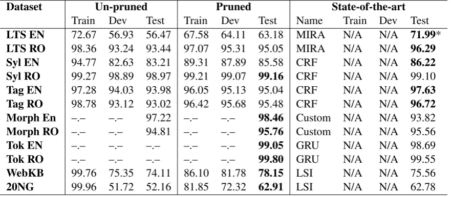
4.3 Accuracy-Boost Using Tree-Pruning
To prove that our tree pruning strategy is effec-tive on real life data, in what follows we are going to compare the accuracy of the un-pruned trees to that of pruned trees. For reference, we are also going to report the highest accuracy of any other state-of-the-art method, provided that the testing conditions are identical. Table3 summarizes the results and, as can be seen, the results obtained using the pruned tree are significantly better that the un-pruned version and are very close to state-of-the-art results reported by other authors. The notable difference on the tagging set between the ID3 classifier and the CRF is mostly influenced by the fact that the CRF implementation generates la-bel bi-grams and uses a Viterbi decoder to select an optimal state sequence. A similar approach can also be obtained using the ID3 tree, but the tree-pruning part would require a different methodol-ogy for computation and optimization and it was currently out-of-scope. However, when it comes to morphology extracted from local word features, the ID3 implementation is closer to the CRF re-sults, mainly because morphologic attribute reso-lution is not influenced by bi-grams (we are not saying that there are no context dependencies be-tween the attributes of words - we imply that these dependencies are not easily handled by the simple use of label bi-grams).
*The results reported in Jiampojamarn et al.
(2008) are probably obtained using a different split or corpora preparation (filtering) procedure. In practice when we tried to reproduce the results with an identical feature template, using the same classifier, we only achieved a 65.19% accuracy on our test-set.
Table 3: Accuracy figures for the selected datasets, reported for the pruned, un-pruned and reference state-of-the-art methods and algorithms
Dataset Un-pruned Pruned State-of-the-art
Train Dev Test Train Dev Test Name Train Dev Test
LTS EN 72.67 56.93 56.47 67.58 64.11 63.18 MIRA N/A N/A 71.99*
LTS RO 98.36 93.24 93.44 97.07 95.31 95.05 MIRA N/A N/A 96.29 Syl EN 94.77 82.63 83.21 89.31 87.89 85.58 CRF N/A N/A 86.22 Syl RO 99.27 98.89 98.97 99.21 99.07 99.16 CRF N/A N/A 99.10
Tag EN 97.28 94.03 93.98 96.05 95.13 95.04 CRF N/A N/A 97.63 Tag RO 98.78 93.12 93.02 96.42 95.68 95.48 CRF N/A N/A 96.72 Morph En –.– –.– 97.22 –.– –.– 98.46 Custom N/A N/A 93.82
Morph RO –.– –.– 94.81 –.– –.– 95.76 Custom N/A N/A 95.56
Tok EN –.– –.– –.– –.– –.– 99.05 GRU N/A N/A 98.69
Tok RO –.– –.– –.– –.– –.– 99.80 GRU N/A N/A 99.55
WebKB 99.76 75.35 74.11 86.10 81.78 78.15 LSI N/A N/A 75.56
20NG 99.96 51.72 52.16 81.85 72.32 62.91 LSI N/A N/A 62.78
Because the current version of the UD corpus was newly released, there are no official papers that evaluate any state-of-the art methods on the latest release of the corpora. However, in this case we compare the pruned tree results with the re-sults reported on the official UD page (tokeniza-tion - using Gated Recurrent Units (GRUs) (Straka et al., 2016)). Also, we were unable to evaluate tokenization results in a “static manner”, because token boundaries for a given character index de-pend on the previously generated breaks. Thus, we only provide the final evaluation results over the test set. Also, we must mention that in order to keep the testing conditions similar to previously reported results we did not alter the tests sets in any way and we used 10% of the original training data for building our development sets.
The state-of-the-art results obtained for WebKB and 20NG are based Latent Semantic Indexing (LSI) (Zelikovitz and Hirsh,2001).
5 Conclusions and Future Work
We introduced our optimized version of the ID3 tree-computation algorithm, as well as a method to fine-tune an existing tree using a development set to selectively prune it. The later mentioned al-gorithm is also optimized for speed using a result-caching approach.
We showed that by fine-tuning a tree structure one can achieve results comparable to state-of-the art classifiers. We argue that decision trees can be easily used in the feature selection process of any machine learning algorithm. Combined with
the enhanced computation time and tree-pruning methodology make this a useful contribution, es-pecially in the field of natural language processing where working with discrete features in a bag-of-words fashion is common.
Additionally, the results reported in section4.3
are obtained by simply extracting features inside the context-window and not by introducing any predefined feature-sets. This is not the case for the state-of-the art results to which we compared our system to, where the features are actually the result of complex careful crafting of feature templates. The robust principles behind decision trees do not require an extensive feature engineering pro-cess. Instead, the constructed tree can offer a good overview of the task and dataset itself and can ac-tually guide the process of constructing feature templates for other classifiers. Finally, one very important note about this implementation is that it was used during the preparation of a shared task which involved more that 50 datasets on which various tasks had to be performed. The enhanced speed of this algorithm allowed us to make over 1000 training runs and explore a rich set of fea-tures, in the short available time, which, without the optimization would otherwise had been impos-sible.
Our implementation of the enhanced ID3 algo-rithm is written in C++ and we provide a JAVA library for the tree-pruning and prediction algo-rithms. The tool is freely available and can be downloaded3.
References
Susan Bartlett, Grzegorz Kondrak, and Colin Cherry. 2008. Automatic syllabification with structured
svms for letter-to-phoneme conversion. In ACL.
pages 568–576.
Mark Craven, Andrew McCallum, Dan PiPasquo, Tom Mitchell, and Dayne Freitag. 1998. Learning to ex-tract symbolic knowledge from the world wide web. Technical report, DTIC Document.
Wei Dai and Wei Ji. 2014. A mapreduce
implemen-tation of c4. 5 decision tree algorithm.
Interna-tional Journal of Database Theory and Application
7(1):49–60.
Thomas G Dietterich. 2000. An experimental compar-ison of three methods for constructing ensembles of decision trees: Bagging, boosting, and
randomiza-tion. Machine learning40(2):139–157.
Sittichai Jiampojamarn, Colin Cherry, and Grzegorz Kondrak. 2008. Joint processing and discriminative training for letter-to-phoneme conversion. In ACL. pages 905–913.
David D Lewis and Marc Ringuette. 1994. A compar-ison of two learning algorithms for text
categoriza-tion. InThird annual symposium on document
anal-ysis and information retrieval. volume 33, pages 81– 93.
Manish Mehta, Jorma Rissanen, Rakesh Agrawal, et al.
1995. Mdl-based decision tree pruning. In KDD.
volume 21, pages 216–221.
Joakim Nivre, Marie-Catherine de Marneffe, Filip Gin-ter, Yoav Goldberg, Jan Hajic, Christopher D Man-ning, Ryan McDonald, Slav Petrov, Sampo Pyysalo, Natalia Silveira, et al. 2016. Universal dependen-cies v1: A multilingual treebank collection. In Pro-ceedings of the 10th International Conference on Language Resources and Evaluation (LREC 2016). pages 1659–1666.
Vincent Pagel, Kevin Lenzo, and Alan Black. 1998. Letter to sound rules for accented lexicon
compres-sion.arXiv preprint cmp-lg/9808010.
Slav Petrov, Dipanjan Das, and Ryan McDonald. 2011.
A universal part-of-speech tagset. arXiv preprint
arXiv:1104.2086.
J. Ross Quinlan. 1986. Induction of decision trees.
Machine learning1(1):81–106.
J. Ross Quinlan. 1987. Simplifying decision
trees. International journal of man-machine studies
27(3):221–234.
J Ross Quinlan. 1993. C4.5: programs for machine
learning. Elsevier.
Rajeev Rastogi and Kyuseok Shim. 1998. Public: A decision tree classifier that integrates building and
pruning. InVLDB. volume 98, pages 24–27.
Helmut Schmid. 2013. Probabilistic part-ofispeech tagging using decision trees. InNew methods in lan-guage processing. Routledge, page 154.
Adriana Stan, Junichi Yamagishi, Simon King, and Matthew Aylett. 2011. The romanian speech synthe-sis (rss) corpus: Building a high quality hmm-based speech synthesis system using a high sampling rate.
Speech Communication53(3):442–450.
Milan Straka, Jan Hajic, and Jana Strakov´a. 2016. Ud-pipe: Trainable pipeline for processing conll-u files performing tokenization, morphological
anal-ysis, pos tagging and parsing. In Proceedings of
the Tenth International Conference on Language Re-sources and Evaluation (LREC 2016).
Jiang Su and Harry Zhang. 2006. A fast decision tree
learning algorithm. InAAAI. volume 6, pages 500–
505.
Gy¨orgy Szarvas, Rich´ard Farkas, and Andr´as Kocsor. 2006. A multilingual named entity recognition sys-tem using boosting and c4. 5 decision tree learning
algorithms. InInternational Conference on
Discov-ery Science. Springer, pages 267–278.
Robert Weide. 2005. The carnegie mellon pronouncing dictionary [cmudict. 0.6].
Sarah Zelikovitz and Haym Hirsh. 2001. Using lsi for text classification in the presence of background text. InProceedings of the tenth international con-ference on Information and knowledge management. ACM, pages 113–118.
Daniel Zeman. 2008. Reusable tagset conversion using tagset drivers. InLREC.
Heiga Zen, Takashi Nose, Junichi Yamagishi, Shinji Sako, Takashi Masuko, Alan W Black, and Keiichi Tokuda. 2007. The hmm-based speech synthesis
system (hts) version 2.0. InSSW. Citeseer, pages
294–299.
Heiga Zen, Keiichi Tokuda, and Alan W Black. 2009.
Statistical parametric speech synthesis. Speech