Data Cube Approximation and Mining using Probabilistic Modeling
Cyril Goutte1
, Rokia Missaoui2
, Ameur Boujenoui3
1
Interactive Language Technologies, NRC Institute for Information Technology 101, rue St-Jean-Bosco, Gatineau, QC, K1A 0R6, Canada
2D´epartement d’informatique et d’ing´enierie, Universit´e du Qu´ebec en Outaouais C.P. 1250, succ. B, Gatineau, QC, J8X 3X7, Canada
3School of Management, University of Ottawa
136 Jean-Jacques Lussier, Ottawa, ON, K1N 6N5, Canada
[email protected], [email protected], [email protected]
Abstract
On-line Analytical Processing (OLAP) techniques commonly used in data warehouses allow the exploration of data cubes according to different analysis axes (dimensions) and under different ab-straction levels in a dimension hierarchy. However, such techniques are not aimed at mining multidi-mensional data.
Since data cubes are nothing but multi-way tables, we propose to analyze the potential of two probabilistic modeling techniques, namely non-negative multi-way array factorization and log-linear modeling, with the ultimate objective of compressing and mining aggregate and multidimensional values. With the first technique, we compute the set of components that best fit the initial data set and whose superposition coincides with the original data; with the second technique we identify a parsimonious model (i.e., one with a reduced set of parameters), highlight strong associations among dimensions and discover possible outliers in data cells. A real life example will be used to (i) discuss the potential benefits of the modeling output on cube exploration and mining, (ii) show how OLAP queries can be answered in an approximate way, and (iii) illustrate the strengths and limitations of these modeling approaches.
Key Words : data cubes, OLAP, data warehouses, multidimensional data, non-negative multi-way array factorization, log-linear modeling.
1
Introduction
A data warehouse is an integration of consolidated and non volatile data from multiple and possibly het-erogeneous data sources for the purpose of decision support making. It contains a collection of data cubes which can be exploited via online analytical processing (OLAP) operations such as roll-up (increase in the aggregation level) and drill-down (either decrease in the aggregation level or increase in the detail) accord-ing to one or more dimension hierarchies, slice (selection), dice (projection), and pivot (rotation) [10]. In a multidimensional context with a setDof dimensions, a dimension (e.g., location of a company, time) is a descriptive axis for data presentation under several perspectives. A dimension hierarchy contains levels, which organize data into a logical structure (e.g., country, state and city for the location dimension). A member, or modality, of a dimension is one of the data values for a given hierarchy level of that dimension. A fact table (such as Table 1) contains numerical measures and keys relating facts to dimension tables. A cube X =hD, Mi is a visual representation of a fact table, where D is a set of n dimensions of the cube (with associated hierarchies) andM is a corresponding set of measures. For simplicity reasons, we assume thatM is a singleton, and we representXbyX= [xi
1i2...in].
of data, we propose to use two complementary techniques: non-negative multi-way array factorization (NMF) and log-linear modeling (LLM). We highlight their potential in handling some important issues in mining multidimensional and large data, namely data compression, data approximation and data mining. A comparative study of the two techniques is also conducted.
The paper is organized as follows. First, we provide in Section 2 some background about the two selected probabilistic modeling techniques: NMF and LLM. Then, an illustrative and real-life example about cor-porate governance quality in Canadian organizations is described in Section 3 and will serve, in Section 4, to illustrate the potential of the selected techniques for cube mining, exploration and visualization. Sec-tion 5 highlights the advantages and limitaSec-tions of the two techniques. SecSec-tion 6 describes some related work. Conclusion and further work are given in Section 7.
In the sequel we will use the terms contingency table, variable, modality, and table tuple to mean respec-tively data cube, dimension, member, and cube cell in data warehousing terminology.
2
Probabilistic Models
Any statistical modeling technique has two conflicting objectives: (i) finding a concise representation of the data, using a restricted set of parameters, and (ii) providing a faithful description of data, ensuring that the observed data is close to the estimation provided by the model. The challenge is to automatically find a good compromise between these two objectives. The first objective will help reduce both storage space and processing cost, while the second one ensures that the generated model yields accurate answers to queries addressed to the data.
Formally, let us assume in the following that we analyze ann-dimensional cubeX= [xi
1i2...in]. Without loss of generality, and to simplify notations, let us assume thatn= 3, and denote the 3-dimensional cube X= [xijk], where (i, j, k)∈[1. . . I]×[1. . . J]×[1. . . K].
The purpose of the probabilistic models we describe below is to assign a probability, denotedP(i, j, k), to the observation of each tuple (i, j, k). For example, if (i, j, k) refers to theincome,educationandoccupation respectively, thenP(i, j, k) is the probability to observe a particular combination of the (income,education, occupation) modalities in the observed population. Assuming that the data cube records the countsxijk of the observations of each combination of the modalities in the data, the (log) likelihood of a given model
θis:
(1) L=−logP(X|θ) =−X
ijk
xijklogP(i, j, k),
assuming independent and identically distributed observations.
The most flexible, or saturated, model consists of estimating each P(i, j, k) based on the data. The Maximum Likelihood solution for the saturated model is obtained for Pb(i, j, k) = xijk/N, with N =
P
ijkxijkthe total number of observations. The main issue is that there areI×J×K−1 free parameters in that model, i.e., as many adjustable parameters as there are cells in the cube.1 This means that: first, the parameters may be poorly estimated; and second, the model does not provide any “compression” of the data since it just reproduces it without modeling any interesting or systematic effect.
At the other end of the spectrum, one of the simplest models implements theindependence assumption, i.e., all dimensions are independent. In such a case,P(i, j, k) =P(i)P(j)P(k) and we only haveI+J+K−3 free parameters. The maximum likelihood estimates are Pb(i) = Pjkxijk/N, Pb(j) =
P
ikxijk/N and
b
P(k) = Pijxijk/N. That parsimonious model is usually too constrained. For example, due to the independence assumption, it is impossible to model any interaction between dimensions. In other words, the behavior along dimensioniis the same regardless of values j and k, e.g., the distribution ofincome is identical regardless of theeducation andoccupation. This makes theindependence assumption unable to model interesting effects, and often too restrictive in practice.
A useful model will usually be somewhat in between these two extremes. It needs to strike a balance between expressive power and parsimony. A useful model may also be seen as a compressed version of
1
the data trading off size versus approximation error: a good model provides a (lossy) compression of the data cube, which approximates its content. One potential application is that it may be faster to access an approximate version of the cube content through the model, than an exact version through the data cube itself. The quality and relevance of this approximation will be addressed later in Section 4. The quality of the model is also crucially dependent on its complexity. We will also suggest methods to select the appropriate model complexity based on the available data. This may be done for example using likelihood ratio tests [11] or information criteria such as the AIC [1] or BIC [37]. Moreover, the overall process of selecting a parsimonious model in LLM can be handled using backward elimination, forward selection or some variant of these two approaches (see Subsection 2.2).
The two models described below (Sections 2.1 and 2.2) try to reach this balance in different ways. The non-negative multi-way array factorization approach models the data as a mixture of conditionally independent components, the combination of which may model more complicated dependencies between dimensions. Log-linear modeling tries to include only relevant variable interactions (and discard weak interactions), in order to represent dependencies between dimensions in a compact way.
2.1 Non-negative Multi-way Array Factorization
In Non-negative Multi-way array Factorization (or NMF), complexity is gradually added to the model by including components in a mixture model. Each component has conditionally independent dimensions, which means that all observations modeled by this component “behave the same way” along each di-mension. In the framework of probabilistic models, this means that the resulting model is a mixture of multinomial distributions:
(2) P(i, j, k) =
C
X
c=1
P(c)P(i|c)P(j|c)P(k|c)
Each componentc= 1. . . C adds (I−1) + (J −1) + (K−1) + 1 parameters to the model. ForC = 1, this simplifies to the independence assumption, and by varyingC, the complexity of the mixture model increases linearly. Note that although within each component the dimensions are independent, this does not mean that the overall model is independent. It means that the data may be modeled as several homogeneous components. To come back to our previous example, one component may correspond to high income andeducation, and another to lowincome andeducation. All members of the former component will tend to have both highincomeand higheducation, while all members of the latter component will have both lowincome and loweducation. Within each component these dimensions are therefore independent. However, the combination of these two components will clearly reveal a dependency between the level of education and theincome. This is similar to modeling continuous distributions with Gaussian mixtures: although each component is Gaussian, the overall model can in fact approximate any distribution with arbitrary precision.
The probabilistic model in Equation 2 is linked to factorization in the following way. Organizing the “profiles”P(i|c), P(j|c) or P(k|c) as I×C matrix W = [P(c)P(i|c)], J ×C matrix H = [P(j|c)] and
K×CmatrixA= [P(k|c)] respectively, we may rewrite Equation 2 as
(3) 1
NX≈ X
c
Wc⊗Hc⊗Ac,
whereWc,Hc andAc are thec-th columns ofW,H andA.
The observed arrayXis thus approximated by the sum ofCcomponents, each of which is the product of three factors. The estimate from the factorization is denoted byXb =NP
cWc⊗Hc⊗Ac. Note that the first factorWcontains thejoint probability P(i, c) =P(c)P(i|c), while the other factors contain conditional probabilities, P(j|c) and P(k|c). Equivalently, we may keep all factors conditional by appropriately multiplying by a diagonal matrix ofP(c). One advantage of conditional probabilities is that the associated “profiles”, e.g., P(i|c = 1) and P(i|c = 2) may be compared directly, even when the corresponding components (c= 1 and c= 2 in our example) have very different sizes (and, as a consequence, different
P(c)).
ap-proach is therefore a particular case ofNon-negative Multi-way array Factorization, or NMF,2cf. [42, 32]. There are two specificities in this probabilistic model. First, the factors are not only positive, they form probabilities. This means that their content (forW) or their columns (forHandA) sum to one. Second, the estimation of the parameters is different. For the probabilistic model, the traditional approach is to rely on Maximum Likelihood estimation. In the context of mixture models, this is conveniently done using the Expectation-Maximization algorithm (EM, [13]). For the more general NMF problem, the ap-proximation in Equation 3 will minimize a divergence between the dataX= [xijk] and the factorization
b
X= [bxijk]. Different expressions of the divergence potentially yield different parameter estimation pro-cedures. However, it turns out that the use of a generalized form of the Kullback-Leibler divergence is actually equivalent to Maximum Likelihood on the probabilistic model. Let us define the Kullback-Leibler divergence as:
(4) KL(X,Xb) =X
i,j,k
(xijklogbxijk−xijk+bxijk)
Going back to the expression of the log-likelihood (Equation 1), and using P(i, j, k) = bxijk, we have
KL(X,Xb) = −L −N +P
ijkbxijk. In addition, it turns out that at the minimum of the divergence,
b
X has the same marginals, and same global sum, as X. As a consequence, minimizing the divergence between the factorization and the observations is exactly equivalent to maximizing the likelihood of the probabilistic model (see also [16] for the 2D case).
One outcome of this equivalence is that in the factorization view, we are not limited to working with an observed arrayXthat contains only integer counts. Any positive3arrayXmay be factorized. This opens the possibility to use NMF directly on data cubes containing for example averages rather than simply frequencies. On the other hand, in the strictly probabilistic formulation,Xcontains counts of observations sampled from a multinomial random variable.4
Another advantage of the factorization setting is that the approximation may be expressed using different costs [40]. For example the squared error divergence, or Frobenius norm,
SE(X,Xb) =X ijk
(xijk−bxijk) 2
will produce a true sparse representation of the data, while the KL divergence will produce many small, but not quite zero, approximations in the array. On the other hand, in the probabilistic view, the parameter estimation typically uses maximum likelihood or penalized versions of it (such as the maximum a posteriori, or MAP, estimate). Other types of costs may be handled after parameter estimation, or using awkward noise models on top of the model in Equation 2.
Parameter estimation: The link between the probabilistic mixture model and NMF also has an im-plication on the parameter estimation procedure. First, it suggests that NMF has many local minima of the divergence. This fact is not widely acknowledged in the NMF literature (for D = 2 or higher). Second, there have been many attempts in statistics to devise strategies that would both stabilize the EM algorithm and promote better maxima. One such approach is the use of deterministic annealing [35].
The parameters of the probabilistic model may be estimated by maximizing the likelihood using the EM algorithm[13, 23]. It turns out that the resulting iterative update rules are almost identical to the NMF update rules for the KL divergence. The details of the iterative EM procedure, and its links to the NMF update rules, are given in Appendix A.
Model selection: The crucial issue in factorization is to select the rank of the factorization, i.e., the number of columns in each factor. Similarly, in mixture modeling, the equivalent problem is to select the proper number of components. This is traditionally done by optimizing various information criteria over the number of components, e.g., AIC [1], BIC [37], NEC [5] or ICL [6]. Note that a mixture of multinomial
2
This generalizes the 2-dimensional Non-negativeMatrixFactorization[27].
3
In fact, one can even compute a NMF of an array with negative values, although the best non-negative approximation of negative values will obviously be 0—and the KL divergence would clearly not work as it is.
4
does not really fit the assumptions behind these criteria. However, as an approximate answer, we will rely on the first two information criteria. In the context of this study, and to stay coherent with the following section, we will express these criteria in terms of the (log) likelihood ratioG2and a number of degrees of freedomdf. G2is defined as twice the difference in log-likelihood between the fitted, maximum likelihood model for the investigated model structure and the saturated model:
(5) G2
= 2X ijk
xijklog
xijk
b xijk
= 2(KL(X,X)−KL(X,Xb)).
The number of degrees of freedom is the difference in number of free parameters between the fitted model and the saturated model: df=IJK−(I+J+K−2)×C. The two information criteria we consider are:
(6) AIC=G2
−2df and BIC=G2
−df×logN
The value ofC that minimizes either criterion may be considered the “optimal” number of components. Note that BIC tends to favor a smaller number of components than AIC, because the penalty for each component is larger wheneverN ≥8. This effect is especially pronounced with mixtures of multinomial, because both the number of parameters and the number of free cells in the observation table can be very large.
Note that there are a number of issues associated with the use of AIC and BIC for selecting the proper number of components, e.g., model completeness (i.e., whether the model class contains the true model) or underlying assumptions. The optimal number of components selected by these criteria must be viewed as an indication rather than an absolute truth.
2.2 Log-Linear Modeling
Log-linear modeling (or LLM, [25, 11]) is commonly used for the analysis of multi-way contingency tables, i.e., tables of frequencies of categorical variables. Therefore, it seems natural to use LLM to analyze and model data cubes whenever such multidimensional data can be expressed as contingency tables.
Without loss of generality and for simplicity reasons, let us consider a contingency table with three variablesA∈ {a1, . . . ai, . . . aI},B∈ {b1, . . . bj, . . . bJ}andC∈ {c1, . . . ck, . . . cK}, wherexijk is the count of the number of observations for which the three variables have values (ai, bj, ck). The idea behind LLM is to approximate the observed frequenciesxijk by the expected frequenciesbxijk as a linear model in the log domain:
(7) log(bxijk) =λ+λA
i +λBj +λCk +λijAB+λACik +λBCjk +λABCijk
The parameters of the LLM are the lambdas in Equation 7.λis the overall mean and the other parameters represent the effects of a set (or subset) of variables on the cell frequency. For example,λA
i represents the main effects of observing valueaifor variable A, whileλBCjk represents the two-way (or second-order) effect of observingB =bj andC =ck. The model in Equation 7 contains alln-ways effects among A,B, and
C, for 1≤n≤3. It is calledsaturated since it is exactly equivalent to estimating one parameter per cell as discussed earlier in Section 2. In order to make the parameters identifiable, the following constraints (calledeffect coding) are imposed.
X
i
λAi =
X
j
λBj =
X
k
λCk = 0
X
j
λABij =
X
i
λABij =
X
k
λACik =
X
i
λACik =
X
k
λBCjk =
X
j
λBCjk = 0
X k λABC ijk = X j λABC ijk = X i λABC ijk = 0 (8)
{A∗B, A∗C} will denote a hierarchical model containingA∗B andA∗C effects as well as any subset of these (in that case,A, B andC) and the overall mean.
For the saturated model corresponding to a 3-way table, the number of parameters is the sum of the following values:
• 1 for the main effect (overall mean)λ
• (I−1) + (J−1) + (K−1) for the 1-way effect parameters: λA
i ,λBj andλCk.
• (I−1)×(J−1) + (I−1)×(K−1) + (J−1)×(K−1) for the 2-way effect parameters: λAB ij ,λACik andλBC
jk .
• (I−1)×(J−1)×(K−1) for the 3-way effect parameters: λABC ijk .
Assuming for example that the number of categories in A, B, and C is I = 2, J = 3, and K = 4, respectively, the model{A∗B, A∗C}has 15 parameters: 1 for the main effect, (I−1)+(J−1)+(K−1) = 6 for the one-way effects, and (I−1)∗(J−1) + (I−1)∗(K−1) = 8 for the two-way effects.
The reasons for using a hierarchical model are threefold: (i) ease of interpretation, as it would make little sense to include higher-order effects without including the underlying lower-order interactions; (ii) lighter computational burden, as it makes model selection more tractable (see below); (iii) convenience of use of the generated model in aggregation operations, such as roll-up, common in OLAP applications.
Parameter estimation: There are a number of techniques for estimating LLM parameters. The mean-based estimates and variants [22, 36] provide closed-form expressions for the parameters by assuming that the logarithms of the frequencies follow Gaussian distributions with the same variance. Although it offers the convenience of an analytical and explicit expression for the parameter estimates, this assumption is usually unreliable, especially when there are many extreme values, which is precisely one situation of interest. It is therefore more common to rely on iterative maximization of the likelihood. One method for doing this is the Newton-Raphson algorithm [20], a standard unconstrained optimization technique that is implemented in many optimization packages. In the context of modeling frequencies in a multi-way array, another popular technique is the Iterative Proportional Fitting (IPF) procedure [12]. IPF works by iterating over the data and refining the estimated values in each cell of the table while maintaining the marginals. The algorithm is simple to implement and has a number of attractive properties [33]. Note that the SPSS software used in our experiments uses IPF for estimating and selecting hierarchical LLM and Newton-Raphson for general log-linear models.
Model selection: Model selection consists of finding the best compromise between parsimony and ap-proximation, i.e., the model which contains the smallest set of parameters and for which the difference between observed and expected frequencies is not significant. This is a tricky issue because an exhaustive search of the best parsimonious model among the 22n
possible models can be very time-consuming. For example, a 3-dimensional table will give rise to 256 possible models. Although the number of hierarchical models is much smaller (e.g., there are 19 hierarchical models for a 3-way table), exhaustive search is still impractical in most cases.
The discrepancy between the observed cell values,xijk, and the estimated ones,bxijk, is measured either globally or locally (i.e., cell by cell). The global evaluation may be conducted based on the likelihood ratio statistic (or deviance) or the Pearson statistic. The devianceG2is defined according to Equation 5 as twice the difference in log-likelihood between the maximum likelihood model and the saturated model. For nested models, and under the null hypothesis (no difference between the two models), the likelihood ratio approximately follows a chi-square distribution with degrees of freedomdf equal to the number of lambda terms set to zero in the tested model (i.e., the difference between the number of cells and the number of free parameters).
Model selection in LLM is commonly performed usingbackward elimination. Starting from the saturated model, one successively eliminates interactions, as long as the associated increase inG2
be eliminated without a significant increase inG2. Forward selectionproceeds the opposite way, by starting with a small model (generally the independence model) and then adding interactions of increasing order as long as they yield a significant decrease inG2. A combination of both, also called stepwise selection, is used when after each addition in a forward step, one attempts to remove unnecessary interactions using backward elimination. Note however that backward elimination is more straightforward when dealing with hierarchical models and seems to be the preferred method in the LLM literature [11].
The likelihood ratio also allows the comparison of two modelsθ1 andθ2, as long as they arenested, i.e.,
θ2contains all the terms inθ1. The likelihood ratio between the models is G2(θ2, θ1) =G21−G 2
2. Under the null hypothesis of no difference, it is approximately chi-square distributed withdf=df1−df2 degrees of freedom. If the computed ratio is higher than the value ofχ2(1−α, df) for an appropriate significance levelα, thenθ1 is significantly worse thanθ2 and the smaller model is discarded.
Besides stepwise methods, information-theoretic criteria such as the AIC [1] or BIC [37] can be used for model selection. These criteria are computed as in Equation 6, and models are selected by minimizing the criterion. This may also be done using backward elimination or forward selection. Note that in the context of LLM, AIC seems to be preferred [11].
As indicated above, the goodness-of-fit may also be evaluated locally, i.e., for each cell. This can be done by computing the standardized residualsSRijk in each cell (i, j, k) as follows:
SRijk =
xijk−xbijk
p b xijk
A large absolute value of the standardized residual in a given cell is a sign that the selected model may not be appropriate for that cell. It can also be interpreted as signaling an outlier in the data.
3
A Case Study
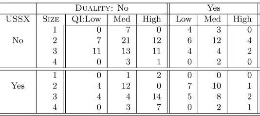
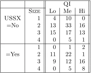
We will now introduce the running example that will be used in the second half of this report to illustrate the use of probabilistic models to integrate Data Mining (DM) and Data Warehousing (DW) technologies. It is based on a study conducted on a sample of 214 Canadian firms listed on the Stock Market and aimed at establishing links between corporate governance practices and other variables such as the shareholding structure [7]. In the context of this study, governance is defined as the means, practices and mechanisms put in place by organizations to ensure that managers are acting in shareholders’ interests. Governance practices include, but are not limited to, the size and the composition of the Board of Directors, the number of independent directors and women sitting on the Board as well as the duality between the position of CEO and the position of Chairman of the Board. The data used in this study were mainly derived from a survey published in October 7, 2002 in the Canadian Globe and Mail newspaper[34], which discussed the quality of governance practices in a sample of firms. More precisely, the mentioned article provided a global evaluation of corporate governance practices of each firm by assessing five governance practices: the composition of the Board of Directors, the shareholding system (or control structure which includes internal shareholders, blockholders and institutional investors), the compensation structure for managers, the shareholding rights and the information sharing system. Data related to the types of shareholding systems, the associated percentage of voting rights and the total assets of each firm were obtained from the “StockGuide 2002” database. Data related to the size of the Board, the number of independent directors and women sitting on the Board, as well as the duality between the position of CEO and the position of Chairman of the Board were extracted from the “Directory of Directors” of the Financial Post. Based on the collected data, a data warehouse has been constructed with sixteen dimensions and an initial set of fact tables for data cube design and exploration. Table 1 is a fact table which provides the number of firms according to four dimensions: USSX,Duality,Size, andQI.USSX∈ {Yes,No}indicates whether the firm is listed or not on a US Stock Exchange. Duality ∈ {Yes,No} indicates whether the CEO is also the Chairman of the Board. Size ∈ {1,2,3,4} represents the size of the firms in terms of the log of their assets. The values are 1 (<2), 2 (≥2 and <3), 3 (≥3 and <4) and 4 (≥4). QIexpresses the index of corporate governance quality (or simply quality index) and takes one of the following values (from worst to best quality): Low (<40%), Medium (≥40 and<70%), and High (≥70%).
Duality: No Yes USSX Size QI:Low Med High Low Med High
1 0 7 0 4 3 0
No 2 7 21 12 6 12 4
3 11 13 11 4 4 2
4 0 3 1 0 2 0
1 0 1 2 0 0 0
Yes 2 4 12 0 7 10 1
3 4 4 14 5 8 2
4 0 3 7 0 2 1
Table 1: Contingency table for the case study: each cell of the 4-dimensional data cube contains the number of companies with the corresponding attributes, according to the four considered dimensions.
with simple statistical techniques [7]. This revealed that the control structure is negatively correlated to the quality of the internal governance mechanisms. In other words, as the concentration of the control mechanisms (i.e., the total shares held by the three types of shareholders) increases, the number of effective internal governance mechanisms sought by an organization decreases. Furthermore, the statistical study showed that internal shareholders and block holders both have a negative impact on the quality of governance while institutional investors have a positive impact. These results, obtained by correlation analysis, were confirmed by a linear regression using the quality index as a dependent variable and taking the control structure and the size of the firm as independent variables. The preliminary statistical analysis helped us construct the most relevant cubes, such that we can focus on mining the most promising tables, i.e., those which contain correlated variables.
4
Experimental Results
In this section, we show and interpret the results produced by NMF and LLM techniques on our case study, illustrated by Table 1.
4.1 NMF results
With the 3×4×2×2 data cube from our case study, each additional component adds 8 parameters to the model. We consider all models from one component, i.e., theindependence model (7 parameters) to five components (39 parameters). For each value of C, we optimize the parameters of the NMF model by maximizing the likelihood. For consistency with the log-linear model, we report results using the likelihood ratio, Equation 5, and calculate AIC and BIC [1, 37] accordingly:
(9) AIC=G2
−2×(48−8×C) and BIC=G2
−(48−8×C) log 47
whereG2 is the likelihood ratio for the maximum likelihood model withC components, 47 is the number of independent cells in the table (the value of the last cell may be deduced from the total cell count), and the number of degrees of freedomdf, as defined in the previous section, is (48−8C).
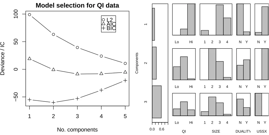
Figure 1 shows that the optimal number of components could be C = 2 or C = 3, with BIC favoring the more parsimonious model. As for the LLM, we rely on the AIC and will therefore focus on the 3-component model. The NMF obtained usingC= 3 components yields estimated frequencies that differ from the observed frequencies on average by ±1.2, with a maximum difference of 4 units (8 estimated vs. 4 observed). This sizable difference is quite unlikely in itself, however, considering that the data cube contains 48 cells, we can expect to observe a few differences that, taken in isolation, have low (sub 5%) probability.
1 2 3 4 5
−50
0
50
100
Model selection for QI data
No. components
Deviance / IC
L2 AIC BIC
3
2
1
Components
0.0 0.6
Lo Hi
Lo Hi
Lo Hi
QI
1 2 3 4
1 2 3 4
1 2 3 4
SIZE
N Y
N Y
N Y
DUALITY N Y
N Y
N Y
USSX
Figure 1: Left: Likelihood ratio, AIC and BIC versus number of components. This suggests thatC= 2 (BIC) or C = 3 (AIC) are reasonable choices for the number of components. Right: Parameters of the 3-component NMF model. The tall, left pane showsP(c); Each row shows P(QI|c), etc., (rescaled) for eachc.
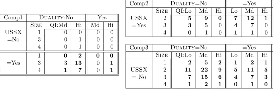
first component obviously corresponds to companies with no duality (i.e., they have distinct CEO and Chairman of the Board), listed in a US Stock Exchange and, as a consequence, with high governance quality. This component thus represents what we could call the “virtuous” companies. Bold numbers in Table 2 represent cells where this componentdominates. For example, a cell (i, j, k) is in bold in the first component if the posterior for this component,P(c = 1|i, j, k) is larger than the posteriors for the other two components.5
This means that companies falling in those cells are more likely to belong to that component than to others.
The second component explains around 27% of the observations. Clearly (see the right side of Figure 1 and Table 2), it corresponds to medium-sized companies (mostlySize=2 or 3) which are listed on a US Stock Exchange (USSX=Yes), yet have medium or low governance quality. These companies predominantly have their CEO as Chairman of the Board, and this seems to impact the governance quality negatively. This is apparent by contrasting theQIpanes for Components 1 and 2 in Figure 1 (top and middle rows).
The last component corresponds to most of the population (59%). It contains only companies not listed in the US (USSX=No). In that way, it is complementary to the first two components which represent all companies listed in the US. The parameters associated with this component are illustrated on Figure 1 (bottom right part) and the corresponding sub-cube is shown in Table 2.
Overall, there is a clear separation between the three components. The first is small and very localized on a subset of modalities corresponding to large and virtuous companies. The second component represents the rest of the companies listed on a US Stock Exchange, for which the governance quality is lower than in Component 1. Finally, the last and largest component contains small to moderate-sized companies which are not listed in the US. This separation corresponds to aclustering of companies into three homogeneous groups.
In addition, all three components are sparse to some extent (81% sparse for Component 1, down to 54% sparse for Component 3). Note, however, that there may be some overlap between the groups (or components). For example, both Component 1 and Component 2 contain companies in cell (QI=Med,
Size=3, Duality=No, USSX=Yes), and both Component 1 and Component 3 are represented in cell (QI=Hi,Size=4,Duality=No, USSX=No).
5
Comp1 Duality:No Yes
Size QI:Md Hi Md Hi
USSX 1 0 0 0 0
=No 3 0 1 0 0
4 0 1 0 0
1 0 2 0 0
=Yes 3 3 13 0 1
4 1 7 0 1
Comp2 Duality=No =Yes
Size QI:Lo Md Hi Lo Md Hi
USSX 2 5 9 0 7 12 1
=Yes 3 3 5 0 4 7 0
4 0 1 0 1 1 0
Comp3 Duality=No =Yes
Size QI:Lo Md Hi Lo Md Hi
1 2 5 2 1 2 1
USSX 2 11 22 9 5 11 5
= No 3 7 15 6 4 7 3
4 1 2 1 0 1 0
Table 2: Components of the 3-component NMF model. Cells where each component dominates are in bold. Cells in non represented rows and columns are uniformly equal to 0.
In summary, NMF identifies (i) a set of homogeneous components, (ii) a number of smaller, locally dense sub-cubes inside a possibly sparse data cube, and (iii) relevant subsets of modalities for each dimension and each component. The user may then explore the data cube by “visiting” the spatially localized sub-cubes associated with each component. Some queries may then be applied only to the components that have the impacted variable modalitites. Other operations like roll-up may be naturally implemented on the probabilistic model by marginalizing the corresponding variables. This is illustrated in Section 4.3 on three kinds of queries.
4.2 LLM results
We recall that the main objectives of probabilistic modeling of data cubes are data compression, approx-imation and mining. A parsimonious probabilistic model may be substituted for the initial data cube in order to provide a faster and more intuitive access to the data, by exhibiting for example the strongest associations discovered by LLM or the components generated by NMF.
Using Table 1 we will now illustrate how a parsimonious log-linear model is selected and how the output of the modeling process can be interpreted. We show also how the selected model and its by-products, such as residuals may be exploited in a data warehouse environment to replace the initial data cube of
n dimensions with a set of data cubes of smaller dimensionality. Finally, we may highlight cells with abnormal values, indicated by high absolute values of standardized residuals.
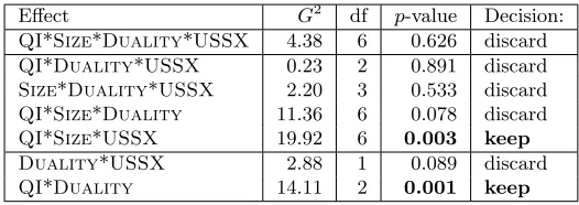
We get a parsimonious model by applyingbackward elimination, as explained in Section 2.2, to the data cube shown on Table 1. Table 3 displays the successive steps in the algorithm. Interactions between variables are tested starting with higher order interactions and in increasing order ofG2. We see that removing the fourth-order effect and all but one third-order effects yields a non-significant difference on the modeling (thep-value from the chi-square test is larger than 5%). Because of the hierarchical model constraint, keepingQI*Size*USSXprevents us from removing the three underlying second-order effects. Out of the three remaining second-order effects,Size*Duality and Duality*USSXmay be removed with no significant loss. Because of the hierarchical model constraint, no first-order effect is candidate for removal as they are all included in the retained second- and third-order effects. As a consequence, the resulting parsimonious model is {QI*Size*USSX, QI*Duality}. The deviance for this model is
G2
= 23.06, with 21 degrees of freedom, which corresponds, according to the chi-square test, to ap-value of 0.341. This means that this parsimonious model is not significantly different from the saturated model in terms of approximation, but it uses only 27 free parameters instead of 48. This is summarized and compared to other models in Table 4.
As the final selected model is{QI∗Size∗USSX,QI∗Duality}, this means that the link betweenQI,
Effect G2
df p-value Decision: QI*Size*Duality*USSX 4.38 6 0.626 discard QI*Duality*USSX 0.23 2 0.891 discard Size*Duality*USSX 2.20 3 0.533 discard QI*Size*Duality 11.36 6 0.078 discard
QI*Size*USSX 19.92 6 0.003 keep
Duality*USSX 2.88 1 0.089 discard QI*Duality 14.11 2 0.001 keep
Table 3: Backward elimination in action: all effects of decreasing order are tested and discarded if their removal does not yield a significant (at the 5% level) decrease in approximation. The resulting model is {QI*Size*USSX,QI*Duality}. For each effect, we report the likelihood ratio statisticG2, the number of degrees of freedomdf, the correspondingp-value (from the χ2 distribution) and the resulting decision.
Model G2 df p-value AIC
1. Independence 98,99 40 0.000 18.99
2. All 2-order terms 42.41 23 0.008 -3.59 3. Parsimonious model 23.06 21 0.341 -18.94
4. All 3-order terms 4.38 6 0.626 -7.62
NMF (best AIC) 39.46 25 n/a -8.54
Table 4: Goodness-of-fit statistics for a set of log-linear models, and comparison with the 3-component NMF. The “parsimonious” model is{QI∗Size∗USSX,QI∗Duality} (see text). The p-value for the NMF is not available as the test only compares models within the same family.
for allSize groups andUSSXvalues.
Table 4 shows that the likelihood ratioG2
for the independence model (Model 1) is high which means that it does not fit the data well. Although this model uses very few parameters, the test shows that the hypothesis that all variables are independent is rejected, i.e., there are associations among the four variables. The model using all second-order effects (Model 2 in Table 4) is also rejected at theα= 0.05 level, which confirms that at least one third-order effect is necessary to fit the data. The remaining models shown in Table 4 have smallerG2and do not depart significantly from the saturated model. Note that we can compare the selected parsimonious model and the “all-3-order” model (Models 3 and 4, respectively, in Table 4) by computing the devianceG2(M odel
4, M odel3) = 23.06−4.38 = 18.68. The corresponding
df is equal to 21-6=15. Since the likelihood ratio statistic is smaller thanχ2(0.95,15) = 25, this suggests that the parsimonious model does not fit the data significantly worse than the “all-3-order” model. As it is more parsimonious, it should be preferred. Using the AIC, the parsimonious model is also the preferred one among the four identified models since its AIC value is the smallest. The 3-parameter NMF indicated for comparison in Table 4 has clearly a worse fit to the data than the best log-linear model. However, because it is slightly more parsimonious, it yields the second best AIC.
The frequencies of the 4-way table, as estimated by the parsimonious log-linear model, are given in Table
Duality: No Yes
USSX Size QI:Low Med High Low Med High
1 2 6 0 2 4 0
No 2 7 20 13 7 13 3
3 8 10 11 8 7 2
4 0 3 1 0 2 0
1 0 1 2 0 0 0
Yes 2 6 13 1 6 9 0
3 5 7 13 5 5 3
4 0 3 7 0 2 1
Table 5: Estimated contingency table for the parsimonious log-linear model {QI∗Size∗USSX,QI∗
QI
Size Lo Me Hi
USSX 1 4 10 0
=No 2 13 33 16
3 15 17 13
4 0 5 1
1 0 1 2
=Yes 2 11 22 1
3 9 12 16
4 0 5 8
Duality
QI: No Yes
Low 26 26
Med 64 41
High 47 10
Table 6: The two sub-cubes identified by LLM as substitutes for the original data cube: QI*Size*USSX, left, andQI*Duality, right.
5. The estimated frequencies are within±3.5 of the data, and within±0.9 on average. The standardized residuals allow to detect unusual departures from expectation, which may indicate outliers or cells that would require further investigation. With this model, the highest standardized residual is 1.969 for the cell that corresponds toQI= High,Size=2,Duality=Yes andUSSX=Yes. This is due to the fact that this is a low-frequency cell in which theresidual is small, but due to the standardization, thestandardized residual becomes borderline significant. None of the cells with higher frequencies display any sizeable standardized residuals.
To sum up, LLM allows us to (i) identify the variables with the most important higher-order interactions, (ii) select a parsimonious model that fits the observed data well with a minimum number of parameters, and (iii) confirm the fit and detect potential outliers using standardized residuals. Whenever the user is interested in conducting a roll-up operation or a simple exploration of the initial cube, then the identified parsimonious model will be used to provide an approximation of the observed data. Moreover, we believe that the highest-order effects can be exploited to notify the user/analyst of the most important associations that hold among dimensions. They can also be used for cube substitution as follows:
• Take the highest-order effects retained by the model selection technique
• Build as many sub-cubes as there are highest-effect terms in the hierarchical parsimonious model.
• Replace the initial data cube with the defined sub-cubes.
4.3 Example queries
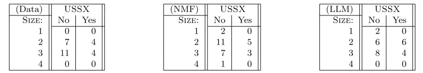
In order to illustrate the impact of the probabilistic models on cube exploration and approximation, let us apply the following OLAP queries to our illustrative example and show how the two models, NMF and LLM, handle them. The first query illustrates the way each probabilistic model may replace the original data cube with smaller and more manageable sub-cubes while the last two queries show dimension selection and a roll-up operation, respectively.
1. Substitution: Counts of firms according toSize,USSX,QIandDuality(the original cube).
2. Selection: Counts according toSizeandUSSX, for firms with low governance quality (QI= Low), where the CEO is not also Chairman of the Board (Duality= No).
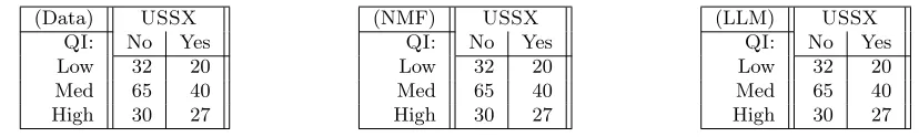
3. Roll-up: Counts of firms according toQIandUSSX, aggregated over all other variables.
(Data) USSX Size: No Yes
1 0 0
2 7 4
3 11 4
4 0 0
(NMF) USSX
Size: No Yes
1 2 0
2 11 5
3 7 3
4 1 0
(LLM) USSX
Size: No Yes
1 2 0
2 6 6
3 8 4
4 0 0
Table 7: Results from the selection query: Size×USSXforQI=Low andDuality=No. Left: Results on original data; Middle: NMF; Right: LLM.
For the 3-component NMF model, the query triggers the visualization of three sub-cubes corresponding to the three components (see Table 2), each representing one cluster. As noted earlier, only a subset of modalities are represented, and the remaining modalities have an estimated count of 0. With minimal loss in approximation, the first component may in fact be represented along USSX and the subset of
Size∈ {3,4}, with the remaining dimensions set toQI=High andDuality=No. The second component is also localized and corresponds to another subset of modalities. With minimal loss of approximation it corresponds to a 3-dimensional cube alongQI∈ {Low, M ed},Size∈ {2,3,4} andDuality, withUSSX
set toY es. Both components are sparse, with only 9 and 12 (respectively) non-zero values out of the original 48 cells, that is 81% and 75% sparsity, respectively (see Table 2). Accordingly, since some rows and columns are zero, this greatly simplifies the description of sub-cubes as locally dense components. The third component is essentially the half of the original cube corresponding to USSX=No. It is less sparse than the first two components, but still less than half the size of the original data cube. Note that although there is some overlap between the sub-cubes corresponding to the three components, most cells are represented in one (and at most two) components. This means that queries involving a subset of modalities may query one or two smaller sub-cubes rather than the original data cube.
The second query is aselection query: for specific modalities of some dimensions, the distribution of the population along the remaining dimensions is sought. In our example, we are interested in characterizing companies which take the virtuous step of keeping their CEO and Chairman separate (Duality=No), yet, have a low governance quality (QI=Low).
For NMF, this query falls outside the range of Component 1. As a consequence, only Components 2 and 3 are invoked. Their values for the relevant cells are simply added to form the answer to the query (Table 7, middle). In LLM, it is necessary to reconstruct the entire data cube from the model, and select data from the estimated cube (Table 7, right). Both models (middle and right) differ somewhat from the original data (left), especially in high frequency cells. The LLM gets a few more cells “right”, but the two active components of the NMF model use only 15 (that is, 8×2−1) parameters while the log-linear model has 27 parameters. This means that NMF trades off a slightly looser fit for increased compression, while the LLM provides better fit but less compression.
Overall, the results of the second query suggest that companies that have low governance quality despite enforcing no duality are medium-sized firms which are typically not listed in a US stock exchange (in about two thirds of cases).
The final query is anaggregation query. It can be answered using LLM by conducting aroll-upoperation on the first sub-cube shown in Table 6. In the case of NMF, and when the sub-cubes generated by LLM are not materialized, we need to compute the overall data cube estimated from the probabilistic model (LLM or NMF) and perform the aggregation specifically. We illustrate this process on theQI×USSX
(Data) USSX QI: No Yes
Low 32 20
Med 65 40
High 30 27
(NMF) USSX
QI: No Yes
Low 32 20
Med 65 40
High 30 27
(LLM) USSX
QI: No Yes
Low 32 20
Med 65 40
High 30 27
Table 8: Aggregation query for the original data cube (left), NMF (middle) and LLM (right): distribution of firms according toQIandUSSX.
(e.g., through a roll-up in a dimension hierarchy).
The results obtained for this last query are identical, and excellent, for both models. As illustrated on Table 8, the link between QIand USSXis weak. There appears to be a slightly higher proportion of “High”QIfor firms withUSSX=Yes versusUSSX=No, but this effect is tenuous at best (compare, e.g., with the link betweenQIandDualityin the second sub-cube in Table 6).
In summary, we can see that NMF provides a slightly more parsimonious model but slightly less precise approximation than LLM. Moreover, thanks to its sparse components, NMF seems more suitable for selection queries while LLM seems more appropriate for aggregation queries. Both LLM and NMF may suggest a substitution of an original data cube into sub-cubes that represent either strong higher-order interactions among dimensions in the case of LLM, or clusters of the initial data within the same set of dimensions in the case of NMF. We elaborate on these differences in the next section.
5
Discussion
Both NMF and LLM offer ways to estimate probabilistic models of a data cube. As such, they share some similarities, e.g., Maximum Likelihood estimation and the need to rely on model selection to optimize the trade-off between approximation and compression. However, they implement this trade-off in different ways. They also display a number of key differences. As a consequence, NMF or LLM may be a better choice in some situation, depending on the type of data and the kind of analysis that is conducted.
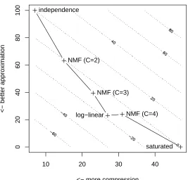
We have seen that essentially all probabilistic models may be positioned between two extremes: the inde-pendencemodel, which offers great compression (i.e., very few parameters) at the expense of approximation quality, and thesaturated model, which simply reproduces the data, hence offers perfect approximation but no compression. In our illustrative example, NMF yields a slightly more parsimonious model than LLM, with 23 versus 27 parameters, but the approximation is not as close—the deviance is 39.46 for NMF and 23.06 for LLM. The trade-off is apparent in Figure 2: theindependenceandsaturated models are two extremes and other probabilistic models are positioned in between. The parsimonious log-linear model has essentially the same deviance as the 4-component NMF, with fewer parameters, hence a better AIC.
As both models are probabilistic models, they associate a probability to each cell in the data cube. This is very helpful to detect outliers by comparing the observed count in one cell with the expected frequency according to the modeled probability. One way to capture this is to compute the standardized residuals. This is commonly done in log-linear modeling packages. Another possibility is to use the fact that both models yield a multinomial probability distribution. One can then compute the probability associated with the count in each cell, according to the model. Outliers correspond to very improbable counts.
10 20 30 40
0
20
40
60
80
100
<− more compression
<− better approximation
independence
NMF (C=2)
NMF (C=3)
log−linear NMF (C=4)
saturated
Figure 2: The compression-approximation trade-off. X-axis is the number of parameters and Y-axis is the likelihood ratio. The dotted lines are contours of the AIC. An ideal model with high compression and excellent approximation would sit in the bottom left corner.
One key difference between both approaches is that LLM focuses on variables, while NMF focuses on modalities. Indeed, for each identified interaction, LLM keeps all modalities of the relevant dimensions. On the contrary, each NMF component keeps all dimensions, but may select some subset of the modalities by setting the probability of the irrelevant modalities to 0. In short, LLM is best at identifying subsets of dimensions, while NMF is best at identifying subsets of modalities. One consequence of this is that NMF can efficiently model sparse data, by placing components on dense regions and setting parameters for the modalities corresponding to empty regions to zero. This is especially interesting for data where some dimensions have a large number of modalities, for example textual data where one dimension may index thousands of words in a vocabulary. On the other hand, LLM is better suited to relatively dense tables. In fact, the usual recommendation [11, 41] for preserving statistical power is to avoid empty cells, have at least five observations per cell for at least 20% of the cells. In addition frequencies for all two-way interactions between variables should be higher than 1.
Although both models can handle a variety of multi-way arrays, there are also key differences in the way they use their parameters. In NMF, the number of parameters scales linearly in the number of components, and the scaling factor is the sum of the number of modalities on all dimensions (up to a small constant, e.g.,I+J+K−2 for three dimensions). On the other hand, the number of parameters in LLM depends on lower-order products of the number of modalities in each of the dimensions involved in the retained interactions. As a consequence, LLM is better suited to modeling tables with many dimensions, each with relatively few modalities, such as high-dimensional data cubes. NMF will get the largest benefits from situations where there are relatively few dimensions, each with large numbers of modalities, such as textual data.
multiplying it by an appropriate constant. However, the application of NMF on data cubes with positive, non integer values is more straightforward and better justified theoretically.
The following table summarizes the strengths and constraints associated with the two studied techniques, and highlights the differences between them.
MODELS Strengths Constraints
Compression Outliers Associations Grouping Sparsity Data size Values
LLM Yes Yes Yes No No >5∗N Counts
NMF Yes Yes No Yes Yes No constr. No constr.
6
Related Work
Many topics have attracted researchers in the area of data warehousing: data warehouse design and multidimensional modeling, materialized view selection, efficient cube computation, query optimization, discovery-driven exploration of cubes, cube reorganization, data mining in cubes, and so on. In order to avoid computing a whole data cube, many studies have focused on iceberg cube calculation [43], partial materialization of data cubes [21], semantic summarization of cubes (e.g., quotient cubes) [26], and approximation of cube computation [38]. Recently, there has been an increasing interest for apply-ing/adapting data mining techniques and advanced statistical analysis (e.g., cluster analysis, principal component analysis, log-linear modeling) for knowledge discovery [30, 31, 36] and data compression pur-poses in data cubes [2, 3, 4, 14]. Our work on log-linear modeling is close to the studies conducted independently by [36, 3, 4, 33]. In [36], an approach based on log-linear modeling (although this is not explicitly stated in their paper) is used to identify exceptions in data cubes by comparing anticipated cell values against actual values. In [3, 4], log-linear modeling is used for data compression. In [33], an approach based on information entropy is used to estimate the original multidimensional data from aggregates and to detect deviations. To that end, the IPF procedure [12] is exploited and its merits are highlighted. We believe that our present work is close to [33] in the sense that we use IPF as the core procedure for parameter estimation of the parsimonious log-linear model and hence for computing original data estimates. LLM also identifies dependencies between variables, and cells which deviate from expected behaviour, as indicated in Section 2.
The NMF approach was developed for factorizing two-dimensional data by Lee and Seung [27, 28]. It was applied to various problems in computer vision [27, 8, 19, 18, 29], music transcription [39] or textual data analysis [44, 17]. The related probabilistic model was developed independently by Hofmann [23] asProbabilistic Latent Semantic Analysis (PLSA). It was used extensively for analyzing textual data in various contexts, e.g., [23, 15, 24]. Some connections between NMF and PLSA were suggested by [9] in the context of multinomial PCA models, and a close relationship was exhibited in [16]. The extension to arrays with more that two dimensions was later introduced by Welling and Weber [42] and applied for example to images or to the decomposition of EEG signal [32]. To the best of our knowledge, Non-negative Multiway-array Factorization has never been applied to the analysis and exploration of data cubes. Our contribution here is to provide such an application, within the more general framework of probabilistic modeling of multidimensional data cubes. We selected the number of factors using a simple AIC criterion. We also discussed some related issues of materialization and the use of the NMF model for various kinds of queries, and highlight its strengths and limitations.
7
Conclusion
In this paper we advocated the use of probabilistic models for the approximation, mining and exploration of data cubes. We have investigated the potential of two probabilistic approaches, log-linear modeling and non-negative multi-way array factorization, and illustrated their use on a real-life, small-scale data set.
LLM) or by relying on information criteria such as the AIC (for both NMF and LLM).
NMF and LLM also provide efficient ways to perform various operations, such as visualization, selection, roll-up or aggregations, on the approximated data. As neither LLM nor NMF is optimally efficient with all of these operations, it makes a lot of sense to consider the results provided by both models. Finally, as both models are probabilistic models, they associate a probability to each cell in the data cube. This is very helpful to detect outliers by comparing the observed count in one cell with the expected frequency according to the modeled probability.
We also showed that NMF and LLM have significant differences. NMF can locate homogeneous dense regions inside a sparse data cube and identifyrelevant modalitieswithin each dimension for each sub cube. LLM, on the other hand, can identifyimportant interactions between subsets of the dimensions. While NMF expresses the original data cube as asuperposition of several homogeneous sub-cubes, so that the user may focus on one particular group at a time rather than the population as a whole, LLM expresses the original data cube as adecomposition containing only strong interactions between variables, so that the user may discard weak interactions from the working space.
Both models break down a complex data analysis problem into a set of smaller sub-problems. In the context of data warehousing, this means that instead of exploring a large multi-dimensional data cube, the user can analyze a few smaller cubes. This reduces distracting and irrelevant elements and eases the extraction of actionable knowledge.
To sum up, the two modeling techniques allow users to (i) focus on relevant parts of the data in order to better conduct analysis and mining tasks and discover new knowledge from the data, (ii) identify the necessary dimensions for explaining various effects in the data, and discard irrelevant variables, and (iii) provide a pertinent characterization of the population, both locally and globally.
Our future work concerns the following topics:
• improving the efficiency of the model selection and parameter estimation procedures in order to scale up to very large data cubes,
• incrementally updating a model obtained from either LLM or NMF when a set of aggregate values are added to the data cube, e.g., a new dimension or new members for a dimension, such as sales for a new month; and
• revising the structure of the dimensions, such as their hierarchy or their members based on the output produced by NMF or LLM.
References
[1] Hirotugu Akaike. A new look at the statistical model identification.IEEE Transactions on Automatic Control, 19(6):716–723, 1974.
[2] Brian Babcock, Surajit Chaudhuri, and Gautam Das. Dynamic sample selection for approximate query processing. InSIGMOD ’03: Proceedings of the 2003 ACM SIGMOD international conference on Management of data, pages 539–550, New York, NY, USA, 2003. ACM Press.
[3] Daniel Barbara and Xintao Wu. Using loglinear models to compress datacube. In WAIM ’00: Proceedings of the First International Conference on Web-Age Information Management, pages 311– 322, London, UK, 2000. Springer-Verlag.
[4] Daniel Barbara and Xintao Wu. Loglinear-based quasi cubes. J. Intell. Inf. Syst., 16(3):255–276, 2001.
[5] Christophe Biernacki, Gilles Celeux, and G´erard Govaert. An improvement of the nec criterion for assessing the number of clusters in a mixture model. Pattern Recognition Letter, 20:267–272, 1999.
[7] Ameur Boujenoui and Daniel Z´eghal. Effet de la structure des droits de vote sur la qualit´e des m´ecanismes internes de gouvernance: cas des entreprises canadiennes. Canadian Journal of Admin-istrative Sciences, 23(3):183–201, 2006.
[8] I. Buciu and I. Pitas. Application of non-negative and local non negative matrix factorization to facial expression recognition. InProceedings of the 17th International Conference on Pattern Recognition (ICPR’04) - Volume 1, 2004.
[9] Wray Buntine. Variational extensions to EM and multinomial PCA. InECML’02, pages 23–34, 2002.
[10] Surajit Chaudhuri and Umeshwar Dayal. An overview of data warehousing and olap technology. SIGMOD Rec., 26(1):65–74, 1997.
[11] Ronald Christensen. Log-linear Models. Springer-Verlag, New York, 1997.
[12] W.E. Deming and F.F. Stephan. On a least squares adjustment of a sampled frequency table when the expected marginal total are known. The Annals of Mathematical Statistics, 11(4):427–444, 1940.
[13] A. P. Dempster, N. M. Laird, and D. B. Rubin. Maximum likelihood from incomplete data via the EM algorithm. Journal of the Royal Statistical Society, Series B, 39(1):1–38, 1977.
[14] Venkatesh Ganti, Mong-Li Lee, and Raghu Ramakrishnan. Icicles: Self-tuning samples for approx-imate query answering. In VLDB ’00: Proceedings of the 26th International Conference on Very Large Data Bases, pages 176–187, San Francisco, CA, USA, 2000. Morgan Kaufmann Publishers Inc.
[15] E. Gaussier, C. Goutte, K. Popat, and F. Chen. A hierarchical model for clustering and categorising documents. InAdvances in Information Retrieval, Lecture Notes in Computer Science, pages 229–247. Springer, 2002.
[16] Eric Gaussier and Cyril Goutte. Relation between PLSA and NMF and implications. InSIGIR ’05: Proceedings of the 28th annual international ACM SIGIR conference on Research and development in information retrieval, pages 601–602, New York, NY, USA, 2005. ACM Press.
[17] Cyril Goutte, Kenji Yamada, and Eric Gaussier. Aligning words using matrix factorisation. In ACL’04, pages 503–510, 2004.
[18] D. Guillamet, J. Vitria, and B. Schiele. Introducing a weighted non-negative matrix factorization for image classification. Pattern Recognition Letter, 24(14):2447–2454, 2003.
[19] David Guillamet, Marco Bressan, and Jordi Vitria. A weighted non-negative matrix factorization for local representation. In IEEE Computer Society Conference on Computer Vision and Pattern Recognition, pages 942–947, 2001.
[20] S.J. Haberman. Analysis of qualitative data, Volume 1. Academic Press, New York, 1978.
[21] Venky Harinarayan, Anand Rajaraman, and Jeffrey D. Ullman. Implementing data cubes efficiently. InSIGMOD ’96: Proceedings of the 1996 ACM SIGMOD international conference on Management of data, pages 205–216, New York, NY, USA, 1996. ACM Press.
[22] D.C. Hoaglin, F. Mosteller, and J.W. Tukey. Understanding Robust and Exploratory Data Analysis. John Wiley, New York, USA, 1983.
[23] Thomas Hofmann. Probabilistic latent semantic analysis. InUAI’99, pages 289–296. Morgan Kauf-mann, 1999.
[24] Xin Jin, Yanzan Zhou, and Bamshad Mobasher. Web usage mining based on probabilistic latent semantic analysis. InKDD ’04: Proceedings of the tenth ACM SIGKDD international conference on Knowledge discovery and data mining, pages 197–205, New York, NY, USA, 2004. ACM Press.
[26] Laks V. S. Lakshmanan, Jian Pei, and Yan Zhao. Quotient cube: How to summarize the semantics of a data cube. In Proceedings of the 28th International Conference on Very Large Databases, VLDB, pages 778–789, 2002.
[27] Daniel D. Lee and H. Sebastian Seung. Learning the parts of objects by non-negative matrix factor-ization. Nature, 401:788–791, 1999.
[28] Daniel D. Lee and H. Sebastian Seung. Algorithms for non-negative matrix factorization. InNIPS’13. MIT Press, 2001.
[29] J. S. Lee, D. D. Lee, S. Choi, and D. S. Lee. Application of non-negative matrix factorization to dy-namic positron emission tomography. InProceedings of the International Conference on Independent Component Analysis and Signal Separation (ICA2001), 2001.
[30] Hongjun Lu, Ling Feng, and Jiawei Han. Beyond intratransaction association analysis: mining multidimensional intertransaction association rules. ACM Trans. Inf. Syst., 18(4):423–454, 2000.
[31] Riadh Ben Messaoud, Omar Boussaid, and Sabine Rabas´eda. A new olap aggregation based on the ahc technique. In DOLAP’04: Proceedings of the 7th ACM international workshop on Data warehousing and OLAP, pages 65–72, New York, NY, USA, 2004. ACM Press.
[32] Morten Mørup, Lars Kai Hansen, Josef Parnas, and Sidse M. Arnfred. Decomposing the time-frequency representation of EEG using non-negative matrix and multi-way factorization. Technical report, Informatics and Mathematical Modeling, Technical University of Denmark, 2006.
[33] Themis Palpanas, Nick Koudas, and Alberto Mendelzon. Using datacube aggregates for approxi-mate querying and deviation detection. IEEE Transactions on Knowledge and Data Engineering, 17(11):1465–1477, 2005.
[34] How ROB created the rating system. Globe and Mail, Report on Business, B6, october 7 2006.
[35] K. Rose, E. Gurewwitz, and G. Fox. A deterministic annealing approach to clustering. Pattern Recogn. Letters, 11(9):589–594, 1990.
[36] Sunita Sarawagi, Rakesh Agrawal, and Nimrod Megiddo. Discovery-driven exploration of olap data cubes. In EDBT ’98: Proceedings of the 6th International Conference on Extending Database Tech-nology, pages 168–182, London, UK, 1998. Springer-Verlag.
[37] Gideon Schwartz. Estimating the dimension of a model.The Annals of Statistics, 6(2):461–464, 1978.
[38] J. Shanmugasundaram, U. Fayyad, and P. S. Bradley. Compressed data cubes for olap aggregate query approximation on continuous dimensions. InKDD ’99: Proceedings of the fifth ACM SIGKDD international conference on Knowledge discovery and data mining, pages 223–232. ACM Press, 1999.
[39] P. Smaragdis and J.C. Brown. Non-negative matrix factorization for polyphonic music transcription. In IEEE Workshop on Applications of Signal Processing to Audio and Acoustics, pages 177–180, 2003.
[40] Suvrit Sra and Inderjit S. Dhillon. Nonnegative matrix approximation: Algorithms and applications. Technical report, Dept. of Computer Sciences, The Univ. of Texas at Austin, May 2006.
[41] J.K. Vermunt. Log-linear models, volume Encyclopedia of Statistics in Behavioral Science, pages 1082–1093. Wiley, Chichester, UK, 2005.
[42] Max Welling and Markus Weber. Positive tensor factorization. Pattern Recognition Letters, 22(12):1255–1261, 2001.
[43] Dong Xin, Jiawei Han, Xiaolei Li, and Benjamin W. Wah. Star-cubing: Computing iceberg cubes by top-down and bottom-up integration. InVLDB, 2003.
A
EM algorithm for Non-negative Multi-way Array Factorization
The EM algorithm is an iterative procedure for maximizing the likelihood by alternating two steps until convergence. The E (Expectation) step calculates the probability that each observation belongs to each component at iterationt:
Pt(c|i, j, k) =PPt(c)Pt(i|c)Pt(j|c)Pt(k|c) γPt(γ)Pt(i|γ)Pt(j|γ)Pt(k|γ)
The M (Maximization) step updates the parameters based on these expectations:
Pt+(c) ← 1
N X
ijk
xijkPt(c|i, j, k) (10)
Pt+(i|c) ← 1
N X
jk
xijkPt(c|i, j, k)/Pt+(c) (11)
Pt+(j|c) ← 1
N X
ik
xijkPt(c|i, j, k)/Pt+(c) (12)
Pt+(k|c) ← 1
N X
ij
xijkPt(c|i, j, k)/Pt+(c). (13)
Note that Equations 10-13 ensure that the parameters are probabilities, i.e., PcPt(c) = P
iPt(i|c) =
P
jPt(j|c) =
P
kPt(k|c) = 1. The EM algorithm converges to a (local) maximum of the likelihood. Depending on initial conditions, the resulting parameter estimates may therefore vary. In some cases, the variation will only be up to component permutation (i.e., same likelihood), or correspond to strictly different models (i.e., different likelihood values).
The minimization of the KL divergence may be carried out by the following update. For W = [wic], H= [hjc], A= [akc], the update forWis
(14) wic←
wic
P
jk(hjcakc)
X
jk
xijk(hjcakc)
b xijk
,
and similarly for updatingH andA, by permuting the factors and their indices [42].
The minimization of the SE divergence is obtained using the update:
(15) wic←wic
P
jkxijk(hjcakc)
P
jkbxijk(hjcakc)
.
Again, the updates forHand Aare similar.
By replacing the probabilities by the corresponding matrix entries, P(i, c) = wic, P(j|c) = hjc and