Entropy2019, 21, x; doi: FOR PEER REVIEW www.mdpi.com/journal/entropy
Article
1
Quantized Constant-Q Gabor Atoms for Sparse Binary
2
Representations of Cyber-Physical Signatures
3
Milton A. Garces1,2*
4
1 Infrasound Laboratory, University of Hawaii, Manoa; [email protected]
5
2 RedVox, Inc.; [email protected]
6
* Correspondence: [email protected]
7
Received: 9 July 2020; Accepted: date; Published: date; Last Updated: 20200809
8
Abstract: Increased data acquisition by uncalibrated, heterogeneous digital sensor systems such as
9
smartphones present new challenges. Binary metrics are proposed for the quantification of
cyber-10
physical signal characteristics and features, and a standardized constant-Q variation of the Gabor atom
11
is developed for use with wavelet transforms. Two different CWT reconstruction formulas are
12
presented and tested under different SNR conditions. A sparse superposition of Nth order Gabor atoms
13
worked well against a blast synthetic using the wavelet entropy and an entropy-like parametrization of
14
the SNR as the CWT coefficient-weighting functions. The proposed methods should be well suited for
15
sparse feature extraction and dictionary-based machine learning.
16
Keywords: Gabor atoms; wavelet entropy; binary metrics; acoustics; quantum wavelet
17
18
1. Overture
19
This paper applies the constant-Q standardized Inferno framework of Garces (2013) to the Gabor
20
wavelet and proposes binary metrics for signature characterization. I assume a cyber-physical sensor
21
system converts observables into digital time series data consisting of a combination of signals and noise.
22
A signal of interest can be hypothetically described by sparse representations that define its signature. If
23
its signature characteristics are sufficiently unique and recognizable from those of ambient coherent and
24
incoherent noise, it can be used to identify and classify an object or process.
25
The transformation of diverse digital measurements into robust, scalable, and transportable
26
representations is a prerequisite for signal detection, source localization, and machine learning
27
applications for signature classification. The challenge at hand is to construct sparse signal
28
representations that contain sufficient information for classification. Unambiguous classification can be
29
elusive; measurement artifacts, unexpected signal variability, and non-stationary noise often conspire to
30
add uncertainty to our classifiers. As will be discussed in this paper, information and uncertainty
31
quantification can be substantially simplified when using standardized wavelets and binary metrics.
32
33
2. About Time
34
Oscillatory processes often exhibit spatial and temporal scalability and self-similarity. Although
35
some physical processes scale linearly, many exhibit recurrent patterns that scale logarithmically and are
36
well represented by power laws. Both linear and logarithmic scales can coexist. For example, overtones
37
in harmonic acoustic systems are often linearly spaced in frequency, yet our sense of tone similarity is
38
close to base 2 logarithmic (binary) octave scales. The term octave comes from the eight major notes in
39
12-tone musical notation, which closely repeat in with factors of two. In this paper I will use the term
40
octave and binary interchangeably to denote the base 2 geometric scaling of frequency and time. The
41
mapping between frequency (or pitch) and time (period) is direct for continuous tones, such as musical
42
notes, or statistically stationary oscillations like the orbits of planets. Discrete Fourier transform methods
43
are exceptionally well suited for the interpretation of steady tonal signals with linearly spaced harmonics.
44
The Fourier transform deconstructs oscillations with distinct recurrent time periods into a spectral
45
representation consisting of a set of discrete frequencies. The spectral transformation can be sparse
46
because it removes time as a variable, making it possible to readily reconstruct stable oscillations from a
47
subset of coefficients in the Fourier spectrum.
48
Stable oscillators can be even more succinctly represented by a fundamental frequency or period
49
(exclusive or, they are not independent). For many physical systems, a map can be constructed between
50
the fundamental and its harmonics. Signals where the fundamental and its harmonics (when they exist)
51
are statistically stationary and easily discernible above noise are referred to as the easy continuous wave
52
(CW) problem, or the zeroth (trivial) class of CW problems. The trivial CW problem is well understood
53
and should routinely be used as a speed and performance benchmark for detection and classification
54
algorithms.
55
The plot thickens when temporal variability is introduced in signal or noise. In the first class of CW
56
problems, temporal variability is due to increased broadband or band-limited noise. This is an
57
exceptionally valuable sensitivity exercise for array processing, where noise can be coherent or
58
incoherent across the array aperture. The first class of CW problems is also well understood when noise
59
is normally distributed over a time duration that is a substantial multiple of the signal period in the
60
detection band. However, this class of problems is not as well characterized when noise is not evenly
61
distributed across the signal detection bandpass, and can be particularly inconvenient when noise steps
62
on the fundamental frequency.
63
In the second class of CW problems, temporal variability is introduced by a change in the temporal,
64
spectral, and/or statistical properties of the signal. These changes can be due to aging, failure, motion,
65
communication, or any other change in state. In a simple two-state problem, one may quantify the
66
properties of the first state, the transition period between states, and the properties on the final state. In
67
a multiple-state problem, such as with communication systems, speech, or music, the short-term discrete
68
Fourier transform (STFT) is often used to characterize spectral variability. This can be a complicated class
69
of problems in the presence of noise.
70
If the transition period between states is faster that the characteristic time scale of the initial state,
71
the STFT does not always provide an accurate representation of this transient. For some signals, the details
72
of the transient are not relevant and only the steady states are important. But a new class of signals
73
emerges when the detection of transient anomalies is prioritized.
74
The zeroth class of transient problems consist of delta functions with their integrals and derivatives:
75
instantaneous spikes which do not exist in the natural world but can be readily constructed digitally and
76
routinely used in the evaluation of the impulse response of a system. The first class of transient problems
77
would be more realistic variants of the delta function that may be observed in the wild when a rapid
78
change of state becomes the signal of interest. Just like a single-tone sinusoid may be regarded as the
79
prototype end member for the trivial CW problem, an explosive detonation could be considered as a
80
prototype transient signal source. During an explosion, observations would vary from ambient noise to
81
a brief blast transient that fades back to a possibly perturbed ambient noise state. If the observations were
82
acoustic at some distance from the source, the system would go from quiescence to blast to quiescence,
83
and the transition can be devastatingly fast. In general, poorly-conditioned STFTs provides inadequate
84
representations of brief, rapidly changing signals because the signatures no longer resemble a CW, and
85
so are not well represented by sinusoids. However, since a STFT is a windowed sinusoid, a
well-86
The concept of a windowed sinusoid to represent a transient signal was introduced by Gabor (1946),
88
and later mathematically formalized by others as wavelets. Variants of the Gabor wavelet are presented
89
in the Appendices.
90
The second class of transient problems overlaps with the second class of CW problems. It
91
corresponds to transients of significant durations which could be addressed with STFTs, wavelets, or
92
their combination. Very often a transient is imbedded in a noise field with band-limited harmonic
93
structure. Or the transient itself is a sweep, characterized by a substantial frequency change in the
94
fundamental and its harmonic structure.
95
The primary differences between STFTs and wavelet approaches are that the former uses a linear
96
period mapping and a constant processing window duration and the latter uses geometric pseudo-period
97
mapping and a window duration that scales with the pseudo-period. Whereas in the Fourier framework
98
there is a one-to-one mapping between time and frequency, the wavelet mapping between time scale and
99
frequency can be less evident and depends on the selected wavelet.
100
In this paper I concentrate on developing standardized constant-Q Gabor atoms for the design and
101
evaluation of transportable, sensor-agnostic signal detection, sparse feature extraction, and classification
102
algorithms.
103
3. Quantifying Information in Cyber-Physical Systems
104
Cyber-physical systems (CPS) are algorithm-controlled computer systems with physical inputs and
105
outputs. A typical example of a mobile CPS is a smartphone with a microphone input (sound activation)
106
that outputs a response (speech, music, or signal recognition) to a screen. Cyber-physical Measurement
107
and Signature Intelligence (MASINT) was defined by Pecenak et. al. (2018) and Cai et al. (2019) as an
108
emerging branch that concentrates on phenomena transmitted through cyber-physical devices and their
109
interconnected data networks. For smartphones and other multi-sensor mobile platforms connected to
110
wireless networks, this must include digital noise, bit errors, and latencies internal to the device and its
111
communication channels.
112
Data processed by the cyber part of CPSs are digital and represented as binary digits (bits). Although
113
the precision of the data is initially defined by its their integer symbol length (16, 32, 64 bit, etc.), the data
114
may convert into float equivalents when an algorithms acts on it. For example, consider sound recorded
115
by a smartphone at the standard rate of 48,000 samples per second. A typical sound record may have
16-116
bit resolution, so that its dynamic range in bits is 2-15 to 215 – 1. However, one may only be interested in
117
the lower frequency components of the raw data, so one would implement a lowpass anti-aliasing before
118
decimation. Such filters require double precision (64 bit at the time of this writing) to reduce instability.
119
Therefore the precision of the resulting lowpass filtered data would be float 64. However, the theoretical
120
dynamic range of the system would not exceed the specification of the integer 16 physical input.
121
Furthermore, data compression can be more efficient on floats than integers, which leads us to the topic
122
of fractional bits as a measure of CPS amplitude, power, and information.
123
Many of the metrics we used in traditional physical and geophysical systems are inherited from the
124
analog era. The base 10 decibel scale is a measure of power relative to a reference level, and is used
125
extensively in telecommunications, acoustics, and electrical engineering. Let’s estimate the hypothetical
126
dynamic range of a 16-bit microphone record of a sinusoid at full scale. The peak rms amplitude would
127
be
128
129
𝑝!"# #%&'()= 2*+ 2√2
130
All systems have quantization and system noise, and it can have a positive or negative bias. This is
132
not a noise paper; for the sake of illustration, I model the system noise as oscillating around a mean of
133
zero and alternating between -1 and 1,
134
𝑝!"# ',%#- = 2* 2√2
135
136
The theoretical dynamic range of the system in dB for a sinusoid recorded with a 16-bit microphone
137
and sound card combination with a one-bit noise floor could be characterized by the ratio of the power
138
139
10 ∗ 𝑙𝑜𝑔*.+
𝑝!"# #%&'() 𝑝!"# ',%#-,
/
= 20 ∗ 𝑙𝑜𝑔*.[2*0] ≈ 90𝑑𝐵
140
141
Where we have converted a digital response to the legacy base 10 logarithmic system. One
142
advantage of the decibel approach is that it can be compared to the response of the human ear and other
143
analog systems. However, analogue comparisons are not necessary for many cyber physical applications.
144
A more natural unit for CPS is the binary logarithm
145
146
𝑙𝑜𝑔/+
𝑝!"# #%&'()
𝑝!"# ',%#-, = 𝑙𝑜𝑔/[2
*0] ≈ 15.0 𝑓𝑏𝑖𝑡𝑠
147
148
Where the unit fbits corresponds to floating point representation of bits. For example, in 24-bit
149
systems, present-day quantization error is ~3 bits, leading to an effective dynamic range of ~21 fbits.
150
Likewise, a 24-bit integer cast into a 32-bit symbol can have 8+3 bits of noise, and may be converted to a
151
float that still has ~21 fbits of dynamic range.
152
Another unit that is often specified is the ½ power point of the frequency response of a filter, which
153
defines the quality factor of that filter. This is often referred to as the -3dB point, since 10 ∗ 𝑙𝑜𝑔*.(2)~3𝑑𝐵.
154
However, accurate filter bank reproductions require a clear specification of the ½ power point, and
155
conversion from base 10 to base 2 specification can lead to computational errors. Plotting filter responses
156
in floating point bits can be informative as it reveals the precision of the computation. Because it is
157
awkward and there is already a precedent in information theory for using bits outside of their original
158
definition as a binary digit, from here onwards in this paper the word bits will be used to represent either
159
the floating point equivalent of bits or as a metric for information.
160
Consider the communication channel capacity introduced by Shannon [1949], which in its simplest
161
form can be expressed as
162
𝐶ℎ = 𝑊𝑙𝑜𝑔/B
𝑆𝑔 + 𝑁𝑠
𝑁𝑠 F
163
164
where 𝐶ℎ is a measure of the differential entropy of a signal in the presence of noise, W is a measure of
165
the bandwidth, 𝑆𝑔 is representative of the power of a signal, and Ns is representative of the noise power.
166
The units of the channel capacity are in shannons, or bits per second, and represents the theoretical upper
167
bound of the rate of information transfer in a communication channel. Since it is often impossible to
168
separate noise already in a signal but it is often possible to construct a noise model, we can think the ratio
169
(Sg+Ns)/Ns as a practical measure of the signal to noise ratio (SNR) of an observed signal that has been
170
carried through a processing system or a medium.
171
The effective SNR and therefore the detectability of a compressed pulse (such as a wavelet) is the
172
product of the bandwidth, the signal to noise ratio, and the duration of a signal T. When using
constant-173
Q Gabor wavelet with fractional octave (binary) bands n of order N and center frequency 𝑓' to process
174
a signal in the presence of noise, I show that for
175
𝑆𝑁𝑅'=𝑁𝑠'+ 𝑆𝑔'
𝑁𝑠' = 1 +
𝑆𝑔' 𝑁𝑠'
177
178
the signal detectability per band can be represented by
179
180
𝑏𝑆𝑁𝑅'=*/ 𝑙𝑜𝑔/(𝑆𝑁𝑅') .
181
182
And the upper limit on rate of information in bits per second for a band-limited pulse with center
183
frequency 𝑓' can be estimated from
184
𝐶ℎ'= 𝑓'
𝑁 𝑏𝑆𝑁𝑅'
185
186
Energy and Shannon entropies using the binary log are constructed for both the wavelet coefficients
187
and SNR in a later section.
188
4. Binary Quantized Constant-Q Gabor Atoms
189
Gabor (1946) extended the Heisenberg principle to define the time-frequency uncertainty principle,
190
and further proposed deconstructing signals into elementary waveforms he referred to as
time-191
frequency atoms (e.g. M09) that provide the optimum compromise between time and frequency
192
resolution and thus maximize information density. Its functional kin, the Morlet wavelet, was
193
developed for seismic applications and is much beloved by mathematicians. Much has been said and
194
written over the last 75 years about the merits, and limitations (e.g. Sheu et al. 2014), of the Gabor atom
195
in diverse fields of applied science ranging from quantum mechanics (e.g. Ashmead 2012),
196
neurophysiology (e.g. Canolty and Womelsdorf, 2019), and radar target recognition (Shi and Zhang,
197
2001). Additional details and references are provided in the Appendixes.
198
The Gabor wavelet atom is a translation and dilation of its familiar mother wavelet
199
Ψ(𝑥) = 1
𝜋*21𝑒𝑥𝑝 L− 𝑥/
2N exp (𝑖Ω3𝑥)
200
with dictionary (M9)
201
Ψ45,'(𝜂) = 1 T𝓈'Ψ L
𝑥 − 𝑥′ 𝓈' N
202
203
Ψ7!,'(𝑡) = 1 𝜋*21
1
T𝓈'𝑒𝑥𝑝 W− 1 2X
𝑥 − 𝑥′ 𝓈' Y
/
Z 𝑒𝑥𝑝 [𝑖Ω3X 𝑥 − 𝑥′
𝓈' Y\
204
205
The constant-q Gabor atoms are constrained to the range of values
206
𝓈'= 𝓈.2 '
3=Ω3
2𝜋 𝑓#𝜏', Ω3= 2√𝑙𝑛2 𝑄3
207
208
with quality factor
209
𝑄3= + 2/3* − 28/3*, 8*
210
211
defined by the ½ power points of the Fourier spectrum. Details of the derivations are provided in
212
214
Ω3/ ≫ 1
215
216
Although in principle 𝑛 ∈ ℤ, 𝑁 ∈ ℝ > 0, for a given bandpass of interest the recommended quanta for
217
the Gabor atoms are positive integer band numbers 𝑛 and the preferred orders 𝑁 as in Garces (2013),
218
219
𝑛 = 0, 1, 2 … , 𝑁 = 1, 3, 6, 12, 24 …
220
221
though the special orders N=0.75 and 1.5 will be considered. The mother wavelet is uniquely defined
222
(and can be quantized) by the order N, although it is often specified by the more accessible variable Ω3.
223
The mother wavelet is scale invariant. Each discrete atom in its dictionary is defined by its order N, its
224
band number n, and a refence scale at n=0. If the Gabor atoms remain within their quanta, there is only
225
one degree of freedom: the reference scale. The reference scale can be set by the data acquisition system
226
(e.g. the Nyquist frequency) or a standard frequency (for example, 1kHz in acoustic applications, 1Hz
227
in infrasound applications). It can also be set by a signal tuning frequency; the peak frequency for a
228
detonation is used in Section 7. When integrating multi-sensor time series with different evenly and
229
unevenly sampled data, it is better to either use a standard reference frequency or time scale (e.g. 1
230
kHz, 1 s, 1 hour) or the target frequency. The resulting bands will be evenly spaced to standardize and
231
facilitate multi-sensor cross-correlations and data fusion. However, it is important to recognize that the
232
mapping from nondimensional scale to physical time scale depends on the sample rate. Inversely,
233
specifying a sample rate 𝑓# or a sample interval ∆𝜏#= 1/𝑓# permits conversion to physical time 𝑡 and
234
time scales 𝜏' in units of the sample interval,
235
𝑡 = 𝑥
𝑓#, 𝓈'= Ω3
2𝜋 𝑓#𝜏', 𝜏'= 𝜏.2 ' 3
236
237
and correspond to the peaks in the Fourier spectrum at the frequencies,
238
239
𝑓'= 𝑓.28 '
3= 1
𝜏', 𝜔'= 2𝜋𝑓'
240
241
It may be useful to think of the binary (base 2) order N as the quantized time and bandwidth stretch
242
factor of the Gabor atom; as the order increases, the wavelet stretches in time and narrows in
243
bandwidth, with each frequency band occupying a constant proportional frequency bandwidth that
244
produces 𝑄3 oscillations at the band frequency in the time domain. As noted a few sentences up in
245
sparser mathematical notation, although in theory it is possible to use any integer band indexes n, the
246
recommended best practice is to use only nonnegative integers to represent temporal scales, with 𝜏.
247
corresponding to the smallest scale and 𝜔. to the highest frequency below the Nyquist frequency.
248
249
The Gabor wavelet and its Morlet kin are attractive to engineers, physicists and mathematicians as
250
they combine two beloved oscillatory and decay functions. They are also popular in information theory
251
as a Gaussian-wrapped oscillation in general, and the Gabor atom in particular, meet the minimal value
252
for the Heisenberg-Gabor uncertainty principle, where the temporal variance 𝜎9/ and angular frequency
253
variance 𝜎:/ over all time and frequency satisfy
254
255
𝜎9𝜎: = 1 2
256
257
This wavelet can be quantized using the well-known fixed order 𝑁 and quality factor 𝑄3 values
258
of standard geometric binary intervals referred to as fractional octave bands in acoustic and infrasound
259
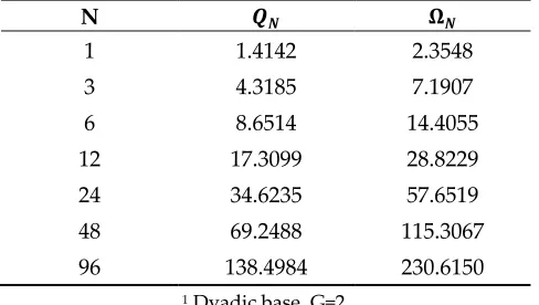
Table 1. Quality factor Q and Ω for standard fractional octave bands of order N 1.
261
N 𝑸𝑵 𝛀𝑵
1 1.4142 2.3548
3 4.3185 7.1907
6 8.6514 14.4055
12 17.3099 28.8229
24 34.6235 57.6519
48 69.2488 115.3067
96 138.4984 230.6150
1 Dyadic base, G=2.
262
Appendix A develops a useful approximation for the quality factor 𝑄3 of order N,
263
264
𝑄3≈ √2𝑁 ≈ 1.414 𝑁, 𝑀3= 2√𝑙𝑛2 𝑄3≈ 2√2𝑙𝑛2 𝑁 ≈ 2.355 𝑁
265
266
with exact equivalence for octave bands at N=1 (Table 2).
267
Table 2. Exact and approximate quality factor Q for standard fractional octave bands of order N 1.
268
N 𝑸𝑵 𝑸𝑵≈ √𝟐𝑵
1 1.4142 1.4142
3 4.3185 4.2426
6 8.6514 8.4853
12 17.3099 16.9706
24 34.6235 33.9411
48 69.2488 67.8823
96 138.4984 135.7645
1 Dyadic base, G=2.
269
270
These relations are seldom made explicit for constant Q wavelet representations, which often leads
271
to inadvertently creative interpretations and implementations. In traditional fractional octave bands, 𝑁
272
is an integer with preferred numbers 1, 3, 6, 12, 24 and its half-power (-3 dB) band edges and center
273
frequencies are well established so their Q can be readily computed (Tables 1 and 2). The band
274
spectrum will overlap at the half-power point band edges to reduce (or at least regulate) spectral
275
leakage and improve energy estimation. Dyadic wavelets use order N=1 and are weakly admissible
276
( Ω3/ ~5.54 ); carefully handled they do lead to very sparse and fast computational implementations
277
(e.g. M9).
278
279
The estimate for 𝑄3 in terms of the order 𝑁 is useful for practical application where we wish to specify
280
the number of oscillations 𝑄3 in a window. If one abandons the bounds of the preferred bands, one can
281
estimate the order for a wavelet that has any number of oscillations in its support window. Once N is
282
estimated, exact values for the center frequencies and band edges can be computed from the expressions
283
in Appendix A. These bespoke constant-Q bands will not meet binary (factor of two) recursions with ½
284
power bandedge overlap, but may be useful for highly customized tuning. Examples are provided in
285
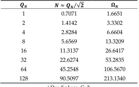
Table 3. Approximate quality factor Q and Ω for non-integer order N 1.
287
𝑸𝑵 𝑵 ≈ 𝑸𝑵⁄√𝟐 𝛀𝑵
1 0.7071 1.6651
2 1.4142 3.3302
4 2.8284 6.6604
8 5.6569 13.3209
16 11.3137 26.6417
32 22.6274 53.2835
64 45.2548 106.5670
128 90.5097 213.1340
1 Dyadic base, G=2.
288
Consider the curious case of a single oscillation in the window, where
289
290
𝑁 =3
4= 0.75, 𝑄3= 1.04, Ω3= 2√𝑙𝑛2 ≈ 1.74
291
292
and Q is evaluated more precisely from the order N. Although intuitive and compact, the resulting
293
wavelets are marginally admissible ( Ω3/ ~3 ) and produce oddly spaced, but legitimate, constant-Q
294
frequency bands that grow rapidly and hit only every fourth standard octave (power of two) every three
295
bands. The window duration will be only 1.74 periods long and the spectral resolution of the Fourier
296
transform will be exceedingly sparse. Adding another oscillation per window (increasing the quality
297
factor to two), would correspond to
298
299
𝑁 =3
2= 1.5, 𝑄3= 2.14, Ω3= 2√𝑙𝑛2 ≈ 3.57
300
301
The resulting wavelets that are more admissible ( Ω3/~12.8 ) but also produced oddly spaced constant-Q
302
frequency bands that land on every second standard octave every three bands. Third order bands hit
303
exact powers of two every third band and have around four oscillations per window (Appendix D).
304
Although it is possible to force center frequency scales, if best practices for band overlap are ignored one
305
will have a set of wavelet filter banks with substantial spectral leakage or gaps between adjacent bands,
306
and the possibility for excessively overdetermined or underdetermines results. This is what usually
307
happens with default parameters on most CWT or DWT algorithms. This paper standardizes and
308
regulates band spacing by asserting the relationship between order, bandwidth, and duration. Since it is
309
both silly and mathematically inadvisable (even inadmissible) to construct a wavelet with less than one
310
oscillation in its window, so it is recommended that 𝑄 ≥ 1. This suggests a minimum order number
311
(quantum) of N=3/4 for stable Gabor atoms, with N=1 yielding value exact power of two (binary) bands.
312
313
It is possible to estimate the smallest possible universal binary scale from the Planck time, the
314
smallest measurable time scale
315
∆𝜏<)('=>= 1081?𝑠 ~ 28*1/𝑠
316
317
Since the Planck time would be the smallest possible sample interval, the smallest oscillation that could
318
be observed would be at the universal Nyquist period
319
320
322
At the other end of the timeline, the age of the universe is estimated to be 13.8 billion years, or
323
𝜏"(7~20@ 𝑠
324
So that the (presently) known universe can be encompassed in the range of ~200 temporal octave bands.
325
Computationally speaking, this is a small range of octaves that can be spanned by 200 temporal Gabor
326
atoms. Earth is estimated to be ~4.6 billion years old, covering around about 57 of those temporal binary
327
bands, and the oldest bones associated with Homo Sapiens-Sapiens are ~200,000 years old and within the
328
last 42 temporal sub-bands since Earth’s inception. The human voice for average individuals ranges
329
between one and two octaves, and five octaves species-wide. A third order representation (N=3) of all
330
the times scales in the universe can be represented by only 600 temporal Gabor atoms. In principle it
331
would be possible to construct universal scales with 𝜏.= 28*1*𝑠, whereas all timescales would occupy
332
temporal sub-bands, but it is not clear there would be practical value to it.
333
334
The beauty of the third order representation is that it is very close to the decimal representation,
335
with every ten 1/3 octaves producing a decade v2*./?~10w, and thus provide a geometrically elegant
336
compromise between ten-digit humans and binary digit machines. In addition to better meeting the
337
admissibility condition, third order bands will contain over 99% of the information within their octave
338
(Appendix E), making them compact temporal carriers. If the third order representation is used as the
339
base order (N=3), the preferred numbers are binary multiples (N = 3, 6, 12, 24 in Table 1), with a
340
proportional elongation in the wavelet support and increase in spectral resolution.
341
342
The nondimensionalized binary scale 𝓈 at the Nyquist frequency is always the same regardless of
343
whether one uses the Plank scale or half the age of the known universe (which would be not only
344
impractical but not very informative as it would only leave one octave to process)
345
𝑄*= √2, Ω*= 2√2𝑙𝑛2, 𝓈.= Ω* 2𝜋
𝜏"%' ∆𝜏<)('=> = x
𝑙𝑛2 2𝜋/
346
𝓈'= 𝓈.2'
347
348
Many software packages readily produce a Gabor-Morlet wavelet with default parameters. One of
349
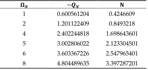
the most common values is Ω3= 5, which is close to order N = 2 (Table 4). Other common values of the
350
wavelet support correspond to Ω3= 4, 𝑁 = 1.7 and the more reasonable Ω3= 8 which is close to
351
preferred order N = 3.
352
Table 4. Approximate quality factor Q and order N for commonly used values of Ω.
353
𝛀𝑵 ~𝑸𝑵 𝐍
1 0.600561204 0.4246609
2 1.201122409 0.8493218
4 2.402244818 1.698643601
5 3.002806022 2.123304501
6 3.603367226 2.547965401
8 4.804489635 3.397287201
1 Dyadic base, G=2.
354
Because none of these specifications correspond to standard orders, the resulting wavelets will tend to
355
either overestimate (due to spectral leakage) or underestimate (due to spectral gaps between bands) the
356
358
Although it is possible to quantize the constant-Q Gabor atoms using the order N, the quality factor
359
Q, or the multiplier Ω, since the lowest recommended order is N=1 it would be more natural to use it to
360
define the quantum order of the wavelet. As the jaded joke goes, naming things is hard. Describing the
361
proposed wavelet dictionaries of preferred orders as the quantized constant-Q Gabor atoms with binary
362
bases and overlapping ½ power points is rather awkward, and this paper I propose referring to these
363
constructs as quantized wavelets, quantum wavelets of order N, or Nth order Gabor atoms. Whether this
364
naming survives the upcoming review process remains to be seen, and the author is open to suggestions.
365
Although N=1 provides the sparsest clean binary (with power of two steps in frequency) representation
366
with the tightest windows, the admissibility condition coupled with the better reconstruction capability
367
presented in the next section suggest that using N=3 as the base order is preferable, with the added
368
advantage that all subsequent preferred orders in Table 1 are binary factors of base order 3.
369
5. Continuous Wavelet Transform Deconstruction and Reconstruction
370
The continuous wavelet transform (CWT) of a function 𝑔(𝑡) is represented in M9 (Eq. 1.13) as
371
372
𝒲(𝑔, 𝑢, 𝓈 ) = 〈𝑔, ΨB,'〉 = • 𝑔(𝑡) 1 √𝓈Ψ
∗B𝑡 − 𝑢 𝓈 F D
8D 𝑑𝑡
373
374
where (*) represents the complex conjugate. The equivalent CWT for a discrete sequence of observations
375
(or a synthetic time series) 𝑔(𝑚) is the convolution of 𝑔 with a scaled and translated version of Ψ(𝑚).
376
Consider the nondimensional Quantum mother wavelet of order N,
377
Ψ3(𝑚) = 1
𝜋*21𝑒𝑥𝑝 L− 𝑚/
2 N exp (𝑖Ω3𝑚)
378
ΨB,'(𝑚) = 1 T𝓈'Ψ3B
𝑚 − 𝑢 𝓈' F
379
𝓈'= Ω3 2𝜋 𝑓#𝜏.2
'
3= 𝓈. 2'3.
380
After M9, define
381
382
Ψ'[𝑚] = 1 T𝓈'Ψ B
𝑚 𝓈'F
383
The discrete CWT can be expressed as
384
385
𝒲'[𝑚] = • 𝑔(𝑚′)Ψ'∗(𝑚′ − 𝑚) EF8*
"!G.
= 𝑔 ⊛ Ψ'∗[𝑚]
386
387
Where the symbol ⊛ denotes a convolution (M9), often computed using the Discrete Fourier transform
388
(Scipy). This is comparable to the expression in Torrence and Compo (1998), although their convolution
389
has no amplitude scaling as it is corrected afterwards. The CWT coefficients 𝒲",' provide a measure of
390
the degree of similarity between the time series and the wavelet of scale index n while translating along
391
the time index m. While exact waveform reconstruction from the CWT is challenging (e.g. Ferges, 1992;
392
Lebedeva and Postnikov, 2014), Torrence and Compo (1998) provide an approximate expression for the
393
wavelet-filtered time series 𝑔′(𝑚). The reconstruction filter from the Nth order Gabor atoms becomes,
394
𝑔[𝑚] ≈𝜋 * 1 𝑁
1 𝐶H •
𝑅𝑒{𝒲'[𝑚]} T𝓈' 3F8*
'G.
396
397
Where Re{ } denotes the real part of the coefficients and the reconstruction factor 𝐶H is scale independent
398
and constant for wavelet function with fixed M3. The reconstruction factor can be estimated by
399
comparing against known test functions. Torrence and Compo (1998) empirically computed a
400
reconstruction coefficient of 𝐶H = 0.776 with M3= 6. Numerical evaluation shows the product 𝑁𝐶H ~2,
401
and the reconstruction approximation for the analytic (Appendix F) quantum wavelet of arbitrary order
402
is
403
404
𝑔ℂ [𝑚] ≈ 𝜋*1
2 •
𝒲'[𝑚] T𝓈' 3F8*
'G.
405
406
It is important to note how substantially different this expression is to the inverse discrete Fourier
407
transform, where
408
𝑔JKL[𝑚] = 1
T𝑁𝑝 • 𝑔†JKL[𝑛] 3F8*
'G.
𝑒𝑥𝑝(𝑗2𝜋𝑚𝑛 𝑁𝑝⁄ )
409
410
where 𝑔†JKL[𝑛] are the Fourier coefficients. Unlike the discrete Fourier transform, the standard wavelet
411
reconstruction does not require multiplication by the mother wavelet. However, in the special case where
412
the atoms are well matched to the signal of interest, it of interest to consider the sparse set of coefficients
413
corresponding the complex time indexes 𝑚' ℂ "(7 of the maximum energy, entropy, or SNR at each scale
414
415
𝑔ℂ [𝑚] ≈ 𝜋*1
2 •
𝒲'[𝑚' ℂ "(7] T𝓈' 3F8*
'G.
𝑅𝑒{Ψ'[𝑚 − 𝑚' ℂ "(7]}
416
417
where the maximum indexes have to be computed separately for real and imaginary components. This
418
has the form of a sum over the dominant Gabor atoms for each scale. Since one is only considering the
419
maxima in a given record window, this is a very sparse representation consisting of the coefficient and
420
the time offset corresponding to the peak energy or entropy estimate. Numerical evaluation shows that
421
this expression can be used to estimate the full analytic function representation as long as reconstruction
422
uses only the real atom function as the time shifts in the Hilbert transform already include the 𝜋/2 time
423
shift.
424
6. Wavelet Information and Entropy
425
One advantage of the constant Q wavelet representation is that it is possible to estimate the
426
information content and detectability of a signal in a band by applying the same set of wavelet transforms
427
to the signal and comparing them to the transform of a noise segment or model. Consider the definition
428
for Shannon’s channel capacity, with
429
430
𝑆𝑁𝑅'=
𝑁𝑠'+ 𝑆𝑔'
𝑁𝑠' = 1 +
𝑆𝑔' 𝑁𝑠'
431
432
𝐶ℎ'= 𝑊𝑙𝑜𝑔/(𝑆𝑁𝑅')
433
where Sg is the wavelet-transformed signal power and Ns is the wavelet-transformed noise power in a
435
band. I consider two possible estimates for the bandwidth W. The first estimate approximates W by the
436
½ power point (-3dB) bandwidth
437
438
∆𝑓'= 𝑓' 𝑄3≈
1 √2
𝑓'
𝑁≈ 0.7071 𝑓' 𝑁
439
440
The second estimates W using the Gabor box standard deviation for the angular frequency
441
442
𝜎:= 1 √2
𝜔' 𝑀3≈
1 4√𝑙𝑛2
𝜔' 𝑁 ≈
𝜋 2√𝑙𝑛2
𝑓'
𝑁≈ 1.8867 𝑓' 𝑁
443
so that
444
𝜎M= 𝜎: 2𝜋 =
1 4√𝑙𝑛2
𝑓'
𝑁 ≈ 0.3003 𝑓' 𝑁
445
446
Taking the average of ∆𝑓' and 𝜎M
447
𝐶ℎ'≈ 1 2
𝑓'
𝑁𝑙𝑜𝑔/(𝑆𝑁𝑅')
448
449
The effective 𝑆𝑁𝑅N and therefore the “detectability” of a bandwidth-limited compressed pulse (Berg
450
and Pellegrino, 1996) can be represented by the product of the Gabor time-bandwidth product (Appendix
451
C) and the signal to noise ratio
452
453
𝑆𝑁𝑅N= 𝜎9 𝜎:× 𝑆𝑁𝑅'
454
455
Since the time-bandwidth product for the Gaussian wavelet is constant
456
457
𝜎9𝜎O= 1 2
458
459
and the uncertainty of its Gabor box is at the minimum, the likelihood of the detection of a SOI in a given
460
band 𝑛 is only proportional to its SNR.
461
Shannon’s definition of the channel capacity was intended to represent the highest theoretical
462
transfer rate of information through an analog line. Since SNR is given in power, which is typically the
463
square of the signal amplitude, an unscaled binary log is off by a factor of two. To reconcile this definition
464
with the original collection of a time series signal in floating point bits (fbits), I define the binary SNR to
465
match the signal rms amplitude as well as Shannon’s units for the information rate per band 𝐶ℎ3,' of
466
the Quantum compressed pulse as
467
468
𝑏𝑆𝑁𝑅'=1
2𝑙𝑜𝑔/(𝑆𝑁𝑅') = 𝑙𝑜𝑔/vT𝑆𝑁𝑅'w, 𝑓𝑏𝑖𝑡𝑠
469
470
𝐶ℎ3,'= 𝑓'
𝑁× 𝑏𝑆𝑁𝑅', 𝑠ℎ𝑎𝑛𝑛𝑜𝑛𝑠 = 𝑓𝑏𝑖𝑡𝑠/𝑠
471
472
The increase in higher information delivery rate with increasing frequency is intuitive as more cycles are
473
transferred per second. As the order number increases, the bandwidth narrows and so the potential
474
information rate decreases. Less obvious is the decrease in high-frequency information with increasing
475
SNR with increasing scaled distance 𝑟 from the source origin on a lossy acoustic channel can be
477
represented as
478
𝑆𝑁𝑅 = 𝑆𝑁𝑅,
𝑒𝑥𝑝(−𝛾𝑓/𝑟) 𝑟'"
479
480
Where 𝑛&= 2 for spherical geometric spreading in free space and 𝑛&= 1 for cylindrical spreading in a
481
waveguide. The binary SNR can be represented as
482
483
𝑆𝑁𝑅 = Œ𝑏𝑆𝑁𝑅.−𝑛&
2 𝑙𝑜𝑔/𝑟 • − 𝑓/𝑟 (𝛾 𝑙𝑜𝑔/𝑒)
484
485
The term in parenthesis shows the expected reduction of one bit per doubling of distance for spherical
486
spreading (𝑛&= 2). The last term suggests the frequency dependence of the channel capacity in a lossy
487
acoustic medium may have the general form
488
489
𝐶ℎ'~ 𝛼(𝑙𝑜𝑔/𝑟) 𝑓 − 𝛽(𝑟) 𝑓?
490
491
so that with increasing range the optimal information transmission frequency shifts to lower frequencies.
492
One may readily extend the binary SNR definition to the measure of relative power
493
494
𝑏𝑅 = 𝑙𝑜𝑔/•x 𝑆 𝑆"(7‘ =
1 2𝑙𝑜𝑔/B
𝑆
𝑆"(7F , 𝑓𝑏𝑖𝑡𝑠
495
496
so that the -3dB half-power point becomes the -1/2 bit power point.
497
The entropy of a signal of interest can be estimated by the wavelet coefficients. A practical approach
498
is described in Li and Zhou (2016). The information content of each scale n at the time step m can be
499
estimated from the wavelet energy. I first estimate
500
501
𝐸",'= “𝑅𝑒” 𝒲",'•“/+ 𝑗 “𝐼𝑚” 𝒲",'•“/
502
503
the total energy in a given record can be estimated from
504
505
𝐸 = • • T𝐸",'𝐸",'∗ '
"
506
507
The probability of 𝒲",' in the record is
508
509
𝑝",'= 𝐸",'
𝐸
510
where
511
512
• • 𝑝",' ' "
𝑝",'∗ = 1
513
514
The log energy entropy (lee) per coefficient can be defined buy the binary logarithm
515
516
𝑒)-- = 𝑙𝑜𝑔/v𝑝",'/ w = 2𝑙𝑜𝑔/v𝑝",'w
517
Where it should be noted that the factor of two scaling coefficient does not alter the relative weight of
519
each coefficient. The Shannon entropy (se) per CWT coefficient is defined as
520
521
𝑒#-= −𝑝",'𝑙𝑜𝑔/v𝑝",'w
522
523
with corresponding complex versions that separate the real and imaginary components. These entropies
524
can be readily evaluated to construct noise models from the lowest entropy components. If a stable noise
525
model can be constructed from the record or from prior knowledge of the environment and transmission
526
channel, SNR estimates can be computed and the process repeated to evaluate the dimensionless binary
527
log of the SNR
528
𝑏𝑆𝑁𝑅",'= 1
2𝑙𝑜𝑔/v𝑆𝑁𝑅",'w
529
530
and the product of the ratio and the binary ratio (RbR), an entropy-like nondimensional metric of the
531
SNR that can be readily evaluated to identify and extract the wavelet coefficients would be most
532
representative of a signal of interest,
533
534
𝑅𝑏𝑅",'= 𝑆𝑁𝑅",'× 𝑏𝑆𝑁𝑅",'
535
7. Praxis: One Ton Blast
536
Consider a normalized transient wave function characteristic of chemical or nuclear explosives.
537
Suppose one wanted to construct a family of wavelets centered around 6.3 Hz, corresponding to the
538
detonation of one metric ton on TNT. It is known that at some distance from the source this center
539
frequency may drop by an octave (factor of two in frequency) or more, as well as become stretched out
540
(dispersed) in time due to propagation effects. A theoretical source pressure function for the detonation
541
of high explosives was developed in some detail in Garces (2019) and is used here to construct a
542
representative synthetic.
543
Let 𝜏̂ =P9 #= 4
9
P$ , where 𝜏= = 4𝜏F is the pseudo-period of a blast pulse corresponding to the peak
544
spectral energy and 𝜏F is the duration of the positive blast phase. The form of the
amplitude-545
normalized source pressure function (Garces 2019) is represented as
546
𝑔(𝜏̂) = (1 − 𝜏̂), 0 ≤ 𝜏̂ ≤ 1
547
𝑔(𝜏̂) =*+(1 − 𝜏̂)v1 + √6 − 𝜏̂w/, 1 < 𝜏̂ ≤ 1 + √6 .
548
This pulse has an associated analytical function 𝑔ℂ(𝜏̂)as discussed in Appendix G. Since the theoretical
549
Hilbert transform has some unresolved issues, I also use the numerical Hilbert transform provided by
550
the Scipy function signal.hilbert for comparison.
551
Note the amplitude is not used in this exercise as in cyber-physical systems such as smartphones the
552
amplitude response of on-board sensors may not be known. However, sensor dynamic range is usually
553
specified and available (e.g. int16, float32) and can be used for signal scaling relative to the full range or
554
the noise.
555
The normalized pulse has zero mean (conservation of momentum) and its theoretical variance is
556
557
𝜎𝑝2 =
"
𝑔2(
𝜏̂)
∞−∞
559
The complex Fourier transform 𝑔†(𝑗𝜔š) of this pulse is
560
561
𝑔†(𝑗𝜔š) = π 2𝜔' œ
1 − 𝑗𝜔š − 𝑒8V:W
𝜔š/ +
𝑒8V:W X*Y√+[
3𝜔š1 ”𝑗𝜔š√6 + 3 + 𝑒V:W √+•3𝜔š/+ 𝑗𝜔š2√6 − 3ž•Ÿ
562
563
where 𝜔š =\/:: $=
P$
1𝜔 = 𝜏F𝜔 and the peak in the spectrum is at 𝜔 = 𝜔= . Note there are at least two
564
pseudoperiods of importance evident in the main blast pulse: the main spectral pseudoperiod 𝜏= and
565
positive phase pseudoperiod of 2𝜏F. Near the source the positive phase pseudoperiod will dominate as
566
it has the highest energy and bandwidth. With increasing distance and high-frequency attenuation the
567
main pseudoperiod becomes more prominent and may also be downshifted in frequency (Garces, 2019).
568
However, additional scales can be introduced by reflection and refraction in the transmission channel
569
that can induce phase shifts often modeled with Hilbert transforms (Appendix G).
570
571
The power spectra of real digital signals are usually expressed using only the positive frequencies
572
up to the Nyquist frequency, where the unilateral spectral density 𝑃𝑔(𝜔š) is defined as
573
574
𝑃𝑔(𝜔š) = 2|𝑔†(𝑗𝜔š)|/= 2 𝑔†(𝑗𝜔š)𝑔†∗(𝑗𝜔š)
575
Since the target signature corresponds to a one tonne (1000 kg) blast, the analysis concentrates on a
576
target frequency of 6.3 Hz (Garces, 2019),
577
𝑓9&= 6.3Hz
578
The general procedure for constructing target-tuned fractional binary bands of order N is to define a set
579
of base-2 scales
580
𝑓V= 𝑓9&2 V 3
581
The upper limit is set by the Nyquist frequency
582
𝑓V "(7 = 𝑓9&2 V "(7
3 <𝑓#
2 ⇒ 𝑗 𝑚𝑎𝑥 < 𝑓𝑙𝑜𝑜𝑟 L𝑁𝑙𝑜𝑔/X 𝑓# 2𝑓9&YN
583
The lower limit is set by the largest data window duration 𝑇
584
𝑓V "%'= 𝑓9&2 V "%'
3 >2
𝑇 ⇒ 𝑗 𝑚𝑖𝑛 > 𝑐𝑒𝑖𝑙 L𝑁𝑙𝑜𝑔/X 2 𝑇𝑓9&YN
585
so the center frequencies are defined by
586
𝑓V= 𝑓9&2 V
3 , 𝑗 ∈ [𝑗 𝑚𝑖𝑛, 𝑗 𝑚𝑎𝑥]
587
which will be sufficient information to compute the Morlet scale 𝓈'. If one must convert to a sorted,
588
monotonically increasing pseudoperiod, let
589
𝜏V= 1
𝑓V, 𝜏.= 𝑚𝑖𝑛v𝜏Vw
590
And restart the counter for the period
591
𝜏'= 𝜏.2 %
&, 𝑛 ∈ [0, 𝑗 𝑚𝑎𝑥 − 𝑗 min = 𝑙𝑒𝑛𝑔𝑡ℎ (𝑓V)]
For the purposes of illustration, let’s choose a signal frequency that exactly matches the target frequency;
594
if this example fails there is no purpose in continuing. This would correspond to
595
596
𝑓== 𝑓9&= 6.3Hz
597
598
in the GT pulse. A sample rate of 200 Hz will be more than sufficient for this example. I add gaussian
599
noise with a standard deviation that is one bit below the signal variance (factor of 1/2), and then
anti-600
alias filter all frequencies below Nyquist. The analytic function is computed numerically from the real
601
pulse for later comparisons with the wavelet-reconstructed signal.
602
The CWT scalogram is computed using the complex nondimensional mother quantum wavelet of
603
order N. The complex Gabor-Morlet wavelet in Scipy is represented by the function scipy.signal.morlet2,
604
and has the desired canonical form,
605
Ψ](𝑚) = 1
𝜋*21𝑒𝑥𝑝 L− 𝑚/
2 N exp (𝑖M3𝑚)
606
ΨB,'(𝑚) = 1 T𝓈'Ψ]B
𝑚 − 𝑢 𝓈' F
607
𝓈'= 𝓈. 2 '
3= +𝑀3
2𝜋𝑓#𝜏., 2 '
3=𝑀3
2𝜋 𝑓# 𝑓'
608
𝑇'= [𝑀3𝜏. ]2 '
3=𝑀3
𝑓'
609
𝑀3= 2T𝑙𝑛(2) 𝑄3
610
𝑄3= + 2 *
/3 − 28/3*, 8*
611
612
The only free variables are the order N, the smallest time scale 𝜏., and the sample rate 𝑓#. The nominal
613
number of points per window can be estimated from 𝑓#𝑇' . The complex wavelet coefficients can be
614
readily computed from the real part of the discrete version of the blast source-time function 𝑝(𝑚)
615
616
𝒲'[𝑚] = • 𝑝(𝑚′)Ψ'∗(𝑚′ − 𝑚) EF8*
"!G.
= 𝑝 ⊛ Ψ'∗[𝑚]
617
618
I use the SciPy cwt function, which in turn invokes the convolution function. This is computationally
619
expensive: we’ve turned a time series with Mp points into a complex 2[Mp x Nbands] array of
band-620
passed waveforms. The terms wavelets and wavelet filter banks are often used interchangeably in the
621
context of the CWT.
622
The wavelet-filtered reconstructed complex analytical signal can be approximated from
623
624
𝑔ℂ %V[𝑚>: 𝑚)] ≈𝜋 * 1 2 •
𝒲'[𝑚>: 𝑚)] T𝓈' V
'G%
625
626
Where the i, j indexes indicate that one may choose selected scales for the reconstruction over selected
627
time indexes 𝑚>: 𝑚) corresponding to the wavelet coefficients that best represent a signal of interest
628
during the time interval of relevance. The scaled wavelet coefficients for an binary band decomposition
629
analytic signal reconstruction (summed over all scales) for the octave band representation. In Figure 1
631
the CWT wavelet amplitudes are scaled by the reconstruction coefficients.
632
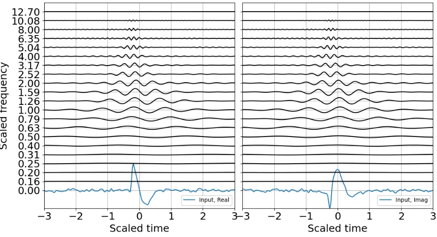
633
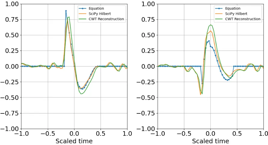
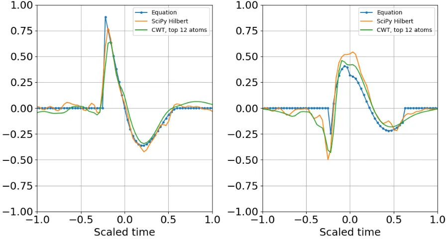
634
Figure 1. Analytical signal from mathematical equation, computation with SciPy Hilbert, and the CWT
635
reconstruction. (a) Real part; (b) imaginary part. The wavelets were evaluated in binary bands (N=1) and
636
constructed around the target frequency of 6.3 Hz, which scales frequency and time. The real input
637
waveform and its computed Hilbert transform are displayed in blue at the zero frequency.
638
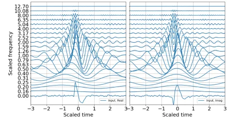
639
Figure 2. Wavelet reconstruction with binary bands. (a) Real part; (b) Imaginary part. The Equation
641
waveform has no noise and is not filtered, whereas Hilbert has Gaussian noise and has been anti-aliased
642
filtered.
643
The reconstruction process recovers the original dimensionality of the time series but returns its Hilbert
644
transform, so the total dimensionality may be doubled (2Mp sample points). If only the original real
645
signal is desired, then the dimensionality is unchanged.
646
647
I next proceed to the estimation of entropy, SNR, and consider sparse signal representation. Although
648
binary bands are adequate for characterizing this signal, and are routinely used in the discrete wavelet
649
transform, I take advantage of the flexibility offered by the CWT and use third order bands (N=3) for the
650
examples that follow. One of the benefits of order 3 bands is that the admissibility condition is better met
651
and scales are recursive in powers of 2 and 10 (e.g. Garces, 2013). As presented in Appendix E, third order
652
bands will contain over 99% of the Gabor box variance within an octave and within 80% of the full
653
window 𝑇', reducing spectral leakage. If, in addition, one wants a factor of two accuracy in explosive
654
yield estimates, 1/3 octave resolution is a minimum requirement. A third order band wavelet
655
decomposition is presented in Figure 3, and is the equivalent of the scalograms usually represented as
656
color plots. I choose the wire mesh representation to better illustrate the simplicity of the CWT
657
decomposition. The difference between Figure 3 and Figure 5 is that the first scales the raw CWT
658
coefficients by the reconstruction scaling, whereas Figure 5 shows the raw coefficients.
659
660
661
Figure 3. Wavelet decomposition with 1/3 octave bands, with CWT amplitudes scaled by the
662
reconstruction coefficients. (a) Real part; (b) Imaginary part. As with Figure 1, the input waveform is
663
displayed at the zero frequency.
665
Figure 4. Wavelet reconstruction with 1/3 octave bands. (a) Real part; (b) Imaginary part.
666
667
668
Figure 5. Wavelet decomposition in order 3 binary bands, raw CWT amplitudes. (a) Real part; (b)
669
Imaginary part.
670
671
The energy probability distribution is constructed from the wavelet coefficients to estimate entropy,
672
add much value, but the Shannon entropy plot is interesting and well scaled (Figure 6). The peak entropy
674
is at the blast center frequency, as expected.
675
676
677
Figure 6. Shannon entropy in order 3 bands from raw CWT amplitudes. (a) Real part; (b) Imaginary part.
678
679
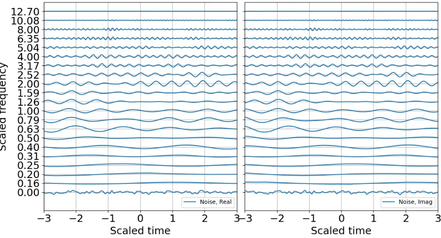
Next I construct a noise model to build the SNR, and to establishing criteria for standardized and
680
reproducible sparse signal representation. Many are the ways to characterize noise, and few of them
681
accurately characterize non-stationary noise over brief observation windows. An incorrect noise model
682
can penalize the signal passband and degrade the signal SNR. For the white noise model with variance
683
that is one bit below the signal variance, the CWT of the noise (Figure 7) shows how the high-frequency
684
oscillations are adequately sampled whereas the low-frequency oscillations are undersampled. This leads
685
to instability if the noise is only estimated over a brief observation record. In principle once can build a
686
noise model over a substantial period of time to obtain better statistical significance under the assumption
687
the noise is stationary. This can be a tenuous assumption in some circumstances. Noise studies are
688
beyond the scope of this paper, and to estimate noise I flatten the noise spectrum by using the mean of
689
the noise coefficients of the over all bands.
690
692
Figure 7. Raw CWT of noise in 1/3 octave bands. (a) Real part; (b) Imaginary part.
693
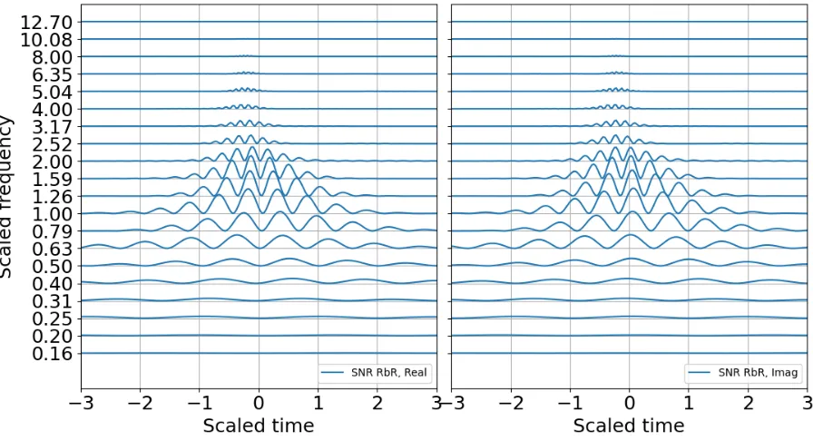
The expected binary SNR would look much like the log energy entropy as they are both scaled by a
694
constant value, the former over the average noise and the latter over the total energy. The SNR RbR, as
695
described in the previous section, should also look very much like the entropy, except it would be zero
696
for SNR of unity and positive for SNR>1. The SNR RbR is shown in Figure 8, and unsurprisingly, matches
697
the Shannon entropy plot. These are good news; the entropy plot requires constructing an energy
698
distribution that scales with the record, whereas the SNR requires constructing a noise model that is
699
mostly independent of the record and should have more stability as long as the ambient noise is
700
approximately stationary or can at least be adequately modeled. If one is curating data for machine
701
learning training, the entropy would be a good metric for picking and annotating, as well as for refining
702
noise models. If one is trying to trigger or detect signals operationally, the SNR may be a preferable metric
703
as it makes no assumptions about the total energy in a record and only scales relative to a (preferably)
704
706
Figure 8. SNR RbR in 1/3 octave bands. (a) Real part; (b) Imaginary part.
707
We can use the CWT coefficient energy, the Shannon entropy, or the SNR RbR test the feasibility of the
708
sparse Gabor atom superposition. Suppose we use any of these Np scales x Mpoint time matrices to
709
identify the peak contributions over the record, and identify the complex time indexes as 𝑚ℂ "(7. The
710
quantum wavelet superposition would be expressed as
711
712
𝑔ℂ %V[𝑚>: 𝑚)] ≈ 𝜋*1
2 •
𝒲'[𝑚' ℂ "(7] T𝓈' V
'G%
𝑅𝑒{Ψ'[𝑚>: 𝑚)− 𝑚' ℂ "(7]}
713
714
where the dimensionality of the representation is reduced to the complex coefficients and time indexes.
715
Since the wavelet function can be reproduced for any time index, the time array need not be stored. In
716
other words, if there are 20 scales, there will be 20 real coefficients and time offsets and 20 imaginary
717
coefficients and time offsets, with total dimensionality of 4x20 = 80 parameters. If there is sufficient SNR
718
and the signal is band limited it is possible to further reduce dimensionality by removing any coefficients
719
below a specified threshold that may be fitting to noise (e.g. overfitting). Figure 9 shows the result of
720
reconstruction from the superposition of all the top atoms of the 20 scales, and Figure 10 shows
721
reconstruction from a sparser set of 12 scales with the highest SNR RbR. Similar results were obtained
722
using the Shannon entropy. The Gaussian noise standard deviation for these two runs was one bit below
723
725
Figure 9. Superposition of largest SNR entropy coefficients per band using all twenty 1/3 octave bands.
726
(a) Real part; (b) Imaginary part. The noise standard deviation is one bit below the signal’s. Dimensionality
727
is reduced to the number of coefficients and their corresponding time shifts.
728
729
Figure 10. Superposition of largest coefficients per band within 4 bits of the peak SNR entropy. (a) Real
730
part; (b) Imaginary part. Dimensionality is further reduced by applying the cutoff.
731
Increasing the noise standard deviation by a factor of two (one bit) still permits reconstruction from
732
734
Figure 11. (a) Real part and (b) imaginary part of the original and reconstructed waveform. Increasing the
735
noise amplitude so that its variance is the same as the signal variance still permitted reconstruction from
736
the superposition of the largest atoms per band.
737
738
Figure 12. (a) Real part and (b) imaginary part of the original and reconstructed waveform. Increasing the
739
noise standard deviation is one bit above the signal standard deviation also allowed reconstruction from
740
the quantum wavelet superposition.
741
There is no end to the number of sensitivity studies that can be performed; in addition to other SNR test
742
Increasing the order past N>6 only worsened the fit to the target waveform so it only increases
744
dimensionality and computational cost with a decrease in reconstruction fidelity, as is to be expected
745
from using a wavelet that does not match the target signature.
746
5. Coda
747
This paper proposes a transition to binary metrics for digital data and introduces a standardized,
748
quantized variation of the Gabor atoms with binary bases, optimal time-frequency resolution, and clear
749
spectral energy containment. A binary entropy-like metric for the SNR is proposed and used to extract
750
the peak coefficients to evaluate the performance of the superposition of Gabor atoms against the more
751
traditional CWT reconstruction. Although the immediate application is the analysis of time series data
752
collected with cyber-physical systems such as smartphones, the methods presented in this paper should
753
be transportable to other types of digital records and can be extended to other wavelet families.
754
I used a synthetic for a 1 tonne detonation in Gaussian noise as an example, and did not include the
755
blast amplitude as a key parameter so as to concentrate on the entropy and SNR, both which are
756
dimensionless scaled quantities. Observations collected close to an explosion should have brief durations
757
and a high SNR; for short pulses it is advisable to use smaller orders (N=1-6) Gabor atoms. Due to cube
758
root yield scaling, the third order bands will provide factor of two yield resolution, and one-sixth order
759
bands a factor of square root of two yield resolution. Acceptable signal reconstructions were obtained
760
from the CWT coefficients as well as the superposition of the peak 3rd order Gabor atoms for the blast
761
signature.
762
At increasing distance from the source the peak frequency is expected to drop (e.g. Garces, 2019)
763
and the pulse disperses to spread out in time. This opens up the possibility for stable 6 and 12 order
764
analyses with a corresponding improvement in yield resolution. Future work will concentrate on such
765
dispersed signatures as well as consider other types of CW signatures that would be well matched to
766
higher-order Gabor atoms.
767
The methods developed have the goal of providing a tunable, standardized framework for signature
768
feature extraction to be used for signal classification (e.g. Shi and Zhang, 2001), and should be well suited
769
for dictionary learning (e.g. M9).
770
771
772
Note to Reviewers:
773
The appendices that follow span over ~5 years and may have different notations than the main body of
774
the text. They are provided as to facilitate verification and will be cleaned up after the review process.
775
Minor modifications since submission have been submitted to preprints.org; they are the result of