University of South Carolina
Scholar Commons
Theses and Dissertations
2016
Some Extremal And Structural Problems In Graph
Theory
Taylor Mitchell Short
University of South Carolina
Follow this and additional works at:https://scholarcommons.sc.edu/etd Part of theMathematics Commons
This Open Access Dissertation is brought to you by Scholar Commons. It has been accepted for inclusion in Theses and Dissertations by an authorized administrator of Scholar Commons. For more information, please [email protected].
Recommended Citation
Some extremal and structural problems in graph theory
by
Taylor Mitchell Short
Bachelor of Science
College of William and Mary 2008
Master of Science
Virginia Commonwealth University 2011
Submitted in Partial Fulfillment of the Requirements
for the Degree of Doctor of Philosophy in
Mathematics
College of Arts and Sciences
University of South Carolina
2016
Accepted by:
László Székely, Major Professor
Éva Czabarka, Committee Member
Linyuan Lu, Committee Member
Csilla Farkas, Committee Member
c
Acknowledgments
First and foremost, thanks to my advisor László Székely. I have learned so much from
not only the lessons you taught me, but also from simply being around you. Thank
you for your patience, support, and inspiration.
Thank you to Éva Czabarka. Your advice has been invaluable. Working closely
with you has been an absolute pleasure.
To Tomislav Došlić, thank you for hosting me during the Summer 2015. Your
kindness and hospitality made my visit to Croatia an experience I will never forget.
This work was partially supported by a SPARC Graduate Research Grant from
the Office of the Vice President for Research at the University of South Carolina and
Abstract
This work considers three main topics. In Chapter 2, we deal with König-Egerváry
graphs. We will give two new characterizations of König-Egerváry graphs as well as
prove a related lower bound for the independence number of a graph. In Chapter 3,
we study joint degree vectors (JDV). A problem arising from statistics is to determine
the maximum number of non-zero elements of a JDV. We provide reasonable lower
and upper bounds for this maximum number. Lastly, in Chapter 4 we study a
problem in chemical graph theory. In particular, we characterize extremal cases for
the number of maximal matchings in two linear polymers of chemical interest: the
polyspiro chains and benzenoid chains. We also enumerate maximal matchings in
several classes of these linear polymers and use the obtained results to determine the
Table of Contents
Acknowledgments . . . iii
Abstract . . . iv
List of Figures . . . vii
Chapter 1 Introduction . . . 1
1.1 König-Egerváry Graphs . . . 1
1.2 Network Models . . . 2
1.3 Chemical Graph Theory . . . 2
Chapter 2 König-Egerváry Theory . . . 4
2.1 Introduction . . . 4
2.2 Some structural lemmas . . . 9
2.3 New characterizations of König-Egerváry graphs . . . 12
2.4 A bound onα(G) . . . 13
Chapter 3 Joint Degree Vectors . . . 14
3.1 Introduction . . . 14
3.2 Definitions and preliminary results . . . 16
3.3 Lower bound construction . . . 18
Chapter 4 Maximal matchings in polyspiro and benzenoid chains 31
4.1 Introduction . . . 31
4.2 Preliminaries . . . 33
4.3 Chain hexagonal cacti . . . 36
4.4 Benzenoid chains . . . 52
4.5 Further developments . . . 71
List of Figures
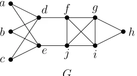
Figure 2.1 Ghas maximum critical independent setI ={a, b, c}. Theorem
2.2 gives that X ={a, b, c, d, e}and Xc ={f, g, h, i, j}. . . . 6
Figure 2.2 G1is a König-Egerváry graph with ker(G1) ={a, b}(core(G1) = nucleus(G1) ={a, b, d}and diadem(G1) = corona(G1) = {a, b, c, d, f}. G2is not a König-Egerváry graph and has ker(G2) = core(G2) = {a, b}(nucleus(G2) ={a, b, d}and diadem(G2) = {a, b, c, d, f}( corona(G) = {a, b, c, d, f, g, h, i, j}. . . 7
Figure 2.3 What theM-alternating paths could look like betweenV(P)∩A and V(P)∩S, where solid lines represent matched edges inM and dotted lines represent the unmatched edges. . . 11
Figure 3.1 The half graph on seven vertices, H7. . . 18
Figure 3.2 A graph on seven vertices that achieves a higher number of non-zero elements in the JDV than the half graph, H7. . . 19
Figure 3.3 An upper bound for the ratio of maximum non-zero elements of the bi-degree vector to its length. . . 21
Figure 3.4 The solution of the discrete and continuous relaxation. The blue line plots the upper bound on αn from Lemma 3.5. The red line is the limit for large n of αn and α0n. . . 21
Figure 4.1 A chain hexagonal cactus of length 6. . . 34
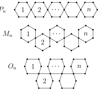
Figure 4.2 The hexagonal cactus chainsPn, Mn, and On. . . 35
Figure 4.3 A benzenoid chain of length 6. . . 35
Figure 4.4 The polyacene, zig-zag polyphenacene, and helicene chains. . . 36
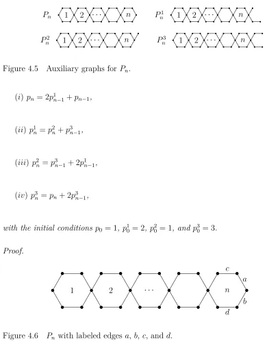
Figure 4.5 Auxiliary graphs forPn. . . 37
Figure 4.7 P1
n with labeled edges a and b. . . 38
Figure 4.8 P2 n with labeled edges a, b, and c. . . 38
Figure 4.9 P3 n with labeled edges a-d. . . 39
Figure 4.10 Auxiliary graphs for Mn. . . 39
Figure 4.11 Mn with labeled edges a-d. . . 40
Figure 4.12 M1 n with labeled edges a and b. . . 40
Figure 4.13 Mn2 with labeled edges a-e. . . 41
Figure 4.14 M3 n with labeled edges a-h. . . 41
Figure 4.15 Auxiliary graphs for On. . . 42
Figure 4.16 On with labeled edges a-d. . . 42
Figure 4.17 O1 n with labeled edges a and b. . . 43
Figure 4.18 O2 n with labeled edges a-e. . . 43
Figure 4.19 On3 with labeled edges a-d. . . 44
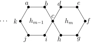
Figure 4.20 A terminal hexagon,hm, and its adjacent hexagon,hm−1, in the hexagonal chain cactusGm. . . 48
Figure 4.21 The hexagonal cactus CP. . . 49
Figure 4.22 The hexagonal cactus CM. . . 50
Figure 4.23 The hexagonal cactus CO. . . 51
Figure 4.24 Auxiliary graphs for Ln. . . 52
Figure 4.25 Ln with labeled edges a-c. . . 53
Figure 4.26 L1n with labeled edges a-e. . . 53
Figure 4.27 L2 n with labeled edges a-d. . . 54
Figure 4.29 Auxiliary graphs for Zn. . . 55
Figure 4.30 Zn with labeled edges a-d. . . 56
Figure 4.31 Z1 n with labeled edges a-g. . . 56
Figure 4.32 Z2 n with labeled edges a-d. . . 57
Figure 4.33 Z3 n with labeled edges a-e. . . 57
Figure 4.34 Z4 n with labeled edges a-f. . . 58
Figure 4.35 Zn5 with labeled edges a-e. . . 59
Figure 4.36 Auxiliary graphs for Hn. . . 59
Figure 4.37 Hn with labeled edges a-e. . . 60
Figure 4.38 Hn1 with labeled edgesa-h. . . 61
Figure 4.39 H2 n with labeled edgesa-i. . . 62
Figure 4.40 H3 n with labeled edgesa and b. . . 63
Figure 4.41 Hn4 with labeled edgesa and b. . . 63
Figure 4.42 H5 n with labeled edgesa-c. . . 64
Figure 4.43 A terminal hexagon,hm, and its adjacent hexagon,hm−1, in the benzenoid chainGm. . . 67
Figure 4.44 The benzenoid chain BL. . . 68
Chapter 1
Introduction
This work concerns the results from [45, 13, 17], each addressing problems from
different areas within graph theory. In this chapter, we give a brief introduction to
the topics considered.
1.1 König-Egerváry Graphs
Every n-vertex, simple graph G satisfies α(G) +µ(G) ≤ n, where α(G) is the
in-dependence number of G and µ(G) is the matching number of G. We say G is a
König-Egerváry graph if α(G) + µ(G) = n. The classical König-Egerváry theorem
implies that every bipartite graph is a König-Egerváry graph, however, there are
non-bipartite graphs which are König-Egerváry as well. Therefore, it is natural to
question whether a characterization of König-Egerváry graphs exists.
Deming [14] was one of the first to work toward a characterization of
König-Egerváry graphs, however, his result only applied to graphs with a perfect matching.
Around the same time, Sterboul [47] produced an equivalent result.
Larson [34] gave a characterization of König-Egerváry graphs involving critical
indepedent sets. Jarden, Levit, and Mandrescu [27, 28] questioned whether a more
global characterization existed, involving unions and intersections of critical
inde-pendent sets. In Chapter 2, we address their questions as well as answer a related
1.2 Network Models
Degree sequences and degree distributions have been subjects of study in graph theory
and many other fields in the past decades. In particular, in social network analysis,
they have been shown to possess a great expressive power in representing and
statis-tically modeling networks.
Joint degree distributions are a generalization of degree distributions that deal
with higher order induced subgraphs than just the nodes of the graph. Different
networks may have the same degree distribution (e.g. scale-free distribution for social
and biological networks) but different assortativity (social networks are assortative
while biological networks are disassortative). Joint degree distributions capture the
assortativity of networks, therefore they are of interest to network scientists.
A special case of the joint degree distribution is the bidegree distribution, which
describes the probability that a randomly selected edge of the graph connects vertices
of degree i andj. However, for this model the general conditions for the existence of
the maximum likelihood estimation (MLE) are not known. As a sufficient condition,
it is known that when there is only one observation of the network available, so
the parameters corresponding to zeros on the bidegree vector are not estimable [43].
This motivates us to find the maximum possible number of non-zero elements on
the bidegree vector of a graph, and consequently the maximum number of estimable
parameters with an observed network. However, this problem seems quite challenging.
In Chapter 3, we provide reasonable lower and upper bounds for this maximum
number.
1.3 Chemical Graph Theory
Chemical graphs are the representation of the structural formula of a chemical
in a graph and the bonds between molecules represented by edges connecting the
vertices (hydrogen-depleted chemical graphs have the hydrogen vertices deleted). For
instance, benzene (molecular formulaC6H6) is an important building block of carbon
nanostructures and is represented by cycle graph on six vertices.
Of particular interest in chemical graphs are enumerative and structural results
of matchings, sets of edges of a graph that do not share a vertex. Matchings most
commonly serve as a model for bonding in chemical molecules. This idea is largely
based on the work of the famous chemist August Kekulé. In 1865, Kekulé [32] claimed
the structure of benzene consisted of a six-membered ring of carbon atoms with
alternating single and double bonds. In the chemical graph of benzene, the edges in
a perfect matching model possible locations for the double bonds. In the chemical
literature, perfect matchings in graphs are also refered to as Kekulé structures.
There is a large and growing literature concerning perfect matchings and
max-imum matchings in chemical graphs, however, maximal matchings are less studied
than their maximum counterparts. Maximal matchings serve as models of adsorption
of dimers to a substrate or a molecule; when that process is random, it is clear that
the substrate can get ‘’clogged‘’ by a number of dimers way below the theoretical
maximum.
In Chapter 4, we consider the number of maximal matchings in two types of
con-nected, plane graphs with underlying hexagonal substructure: hexagonal chain cacti
(also known as polyspiro chains in the chemical literature) and benzenoid chains. In
both types of graphs, every face is a hexagon (except the unbounded one). We
char-acterize extremal structures for the number of maximal matchings in these graphs.
We also enumerate maximal matchings in several classes of these linear polymers and
Chapter 2
König-Egerváry Theory
2.1 Introduction
The König-Egerváry theorem is a classical result in graph theory that states in a
bipartite graph, the size of a maximum matching equals the cardinality of a minimum
vertex cover. For a graph G, let α(G) be the independence number and µ(G) be the
matching number. It is well-known that anyn-vertex graphGsatisfies the inequality
α(G) +µ(G)≤n. (2.1)
The König-Egerváry theorem is equivalent to the statement that equality holds in
(2.1) for all bipartite graphs, however the converse of this statement is not true, see
G1in Figure 2.2 for an example. In 1979, Deming [14] generalized the König-Egerváry
theorem by defining aKönig-Egerváry graph to be a graphGsuch that equality holds
in (2.1). In the same year, Sterboul [47] studied such graphs as well.
In this chapter G is a simple graph with vertex set V(G), |V(G)| = n, and
edge set E(G). The set of neighbors of a vertex v is NG(v) or simply N(v) if there
is no possibility of ambiguity. If X ⊆ V(G), then the set of neighbors of X is
N(X) =∪u∈XN(u),G[X] is the subgraph induced by X, and Xc is the complement
of the subsetX. For sets A, B ⊆V(G), we useA\B to denote the vertices belonging
toAbut notB. For such disjointAand B we let (A, B) denote the set of edges such
that each edge is incident to both a vertex in A and a vertex in B.
A matching M is a set of pairwise non-incident edges of G. A matching of
maxi-mum matching. For a setA⊆V(G) and matchingM, we sayA issaturated byM if
every vertex ofA is incident to an edge inM. For two disjoint setsA, B ⊆V(G), we
say there is a matching M ofA into B if M is a matching of Gsuch that every edge
of M belongs to (A, B) and each vertex ofA is saturated. AnM-alternating path is
a path that alternates between edges in M and those not in M. An M-augmenting
path is an M-alternating path which begins and ends with an edge not in M.
A set S ⊆ V(G) is independent if no two vertices from S are adjacent. An
independent set of maximum cardinality is amaximum independent set and α(G) is
the cardinality of such a maximum independent set. For a graphG, let Ω(G) denote
the family of all its maximum independent sets, let
core(G) =\{S :S ∈Ω(G)}, and corona(G) =[{S:S ∈Ω(G)}.
See [36, 7, 44] for background and properties of core(G) and corona(G).
For a graph G and a set X ⊆V(G), the difference of X is d(X) =|X| − |N(X)|
and the critical difference d(G) is max{d(X) : X ⊆V(G)}. Zhang [52] showed that
max{d(X) : X ⊆ V(G)} = max{d(S) : S ⊆ V(G) is an independent set}. The set
X is a critical set if d(X) = d(G). The set S ⊆ V(G) a critical independent set
if S is both a critical set and independent. A critical independent set of maximum
cardinality is called a maximum critical independent set. Note that for some graphs
the empty set is the only critical independent set, for example odd cycles or complete
graphs. See [52, 9, 35, 34] for more background and properties of critical independent
sets.
Finding a maximum independent set is a well-known NP-hard problem. Zhang
[52] first showed that a critical independent set can be found in polynomial time.
Butenko and Trukhanov [9] showed that every critical independent set is contained
in a maximum independent set, thereby directly connecting the problem of finding a
Returning to consider König-Egerváry graphs, we adopt the convention that the
empty graph K0, without vertices, is a König-Egerváry graph. In [34] it was shown
that König-Egerváry graphs are closely related to critical independent sets.
Theorem 2.1. [34] A graph G is König-Egerváry if, and only if, every maximum
independent set in G is critical.
Theorem 2.2. [34] For any graph G, there is a unique set X ⊆V(G) such that all
of the following hold:
(i) α(G) = α(G[X]) +α(G[Xc]),
(ii) G[X] is a König-Egerváry graph,
(iii) for every non-empty independent set S in G[Xc], |N(S)| ≥ |S|, and
(iv) for every maximum critical indendent set I of G, X =I ∪N(I).
Larson in [35] showed that a maximum critical independent set can be found in
poly-nomial time. So the decomposition in Theorem 2.2 of a graphGintoX andXcis also
computable in polynomial time. Figure 2.1 gives an example of this decomposition,
where both the sets X and Xcare non-empty. Recall, for some graphs the empty set
is the only critical independent set, so for such graphs the set X would be empty. If
a graph G is a König-Egerváry graph, then the set Xc would be empty. We adopt
the convention that if K0 is empty graph, then α(K0) = 0.
G a
b
c
d
e
f g
h
i j
In [37, 28] the following concepts were introduced: for a graph G,
ker(G) =\{S :S is a critical independent set in G},
diadem(G) =[{S :S is a critical independent set in G}, and
nucleus(G) =\{S :S is a maximum critical independent set in G}.
However, the following result due to Larson allows us to use a more suitable definition
for diadem(G).
Theorem 2.3. [35] Each critical independent set is contained in some maximum
critical independent set.
For the remainder of this paper we define
diadem(G) = [{S:S is a maximum critical independent set in G}.
Note that if G is a graph where the empty set is the only critical indepedent set
(in-cluding the caseG=K0, the empty graph), then ker(G),diadem(G), and nucleus(G)
are all empty. See Figure 2.2 for examples of the sets ker(G), diadem(G), and
nucleus(G).
G1
a
b
c
d
e
f
g
G2
a
b
c
d
e
f
g h
i j
Figure 2.2 G1 is a König-Egerváry graph with
ker(G1) = {a, b}(core(G1) = nucleus(G1) = {a, b, d} and
diadem(G1) = corona(G1) ={a, b, c, d, f}. G2 is not a König-Egerváry graph and
has ker(G2) = core(G2) ={a, b}(nucleus(G2) ={a, b, d}and
In [27, 28], the following necessary conditions for König-Egerváry graphs were
given:
Theorem 2.4. [27] If G is a König-Egerváry graph, then
(i) diadem(G) = corona(G), and
(ii) |ker(G)|+|diadem(G)| ≤2α(G).
Theorem 2.5. [28] IfGis a König-Egerváry graph, then|nucleus(G)|+|diadem(G)|=
2α(G).
In [27] it was conjectured that condition (i) of Theorem 2.4 is sufficient for
König-Egerváry graphs and in [28] it was conjectured the necessary condition in Theorem
2.5 is also sufficient. The purpose of this paper is to affirm these conjectures by
proving the following new characterizations of König-Egerváry graphs.
Theorem 2.6. For a graph G, the following are equivalent:
(i) G is a König-Egerváry graph,
(ii) diadem(G) = corona(G), and
(iii) |diadem(G)|+|nucleus(G)|= 2α(G).
The paper [27] gives an upper bound forα(G) in terms of unions and intersections
of maximum independent sets, proving
2α(G)≤ |core(G)|+|corona(G)|
for any graph G. It is natural to ask whether a similar lower bound for α(G) can
be formulated in terms of unions and intersections of critical independent sets.
Jar-den, Levit, and Mandrescu in [27] conjectured that for any graph G, the inequality
|ker(G)|+|diadem(G)| ≤ 2α(G) always holds. We will prove a slightly stronger
statement. By Theorem 2.3 we see that ker(G) ⊆ nucleus(G) holds implying that
|ker(G)|+|diadem(G)| ≤ |nucleus(G)|+|diadem(G)|. In section 2.4 we will prove
Theorem 2.7. For any graph G,
|nucleus(G)|+|diadem(G)| ≤2α(G).
It would be interesting to know whether the sets nucleus(G) and diadem(G), or their
sizes, can be computed in polynomial time.
2.2 Some structural lemmas
Here we prove several lemmas which will be needed in our proofs. Our results hinge
upon the structure of the setX as described in Theorem 2.2.
Lemma 2.8. LetI be a maximum critical independent set inGand setX =I∪N(I).
Then diadem(G)∪N(diadem(G)) =X.
Proof. By Theorem 2.2 the set X is unique in G, that is, for any maximum critical
independent set S,X =S∪N(S). Then diadem(G) = X follows by definition.
Lemma 2.9. LetI be a maximum critical independent set inGand setX =I∪N(I).
Then diadem(G)⊆diadem(G[X]) and nucleus(G[X])⊆nucleus(G).
Proof. LetS be a maximum critical independent set inG. Using Theorem 2.2 we see
that S is a maximum independent set in G[X] and also G[X] is a König-Egerváry
graph. Then Theorem 2.1 gives that S must also be critical in G[X], which implies
that diadem(G)⊆diadem(G[X]).
Now letv ∈nucleus(G[X]). Thenvbelongs to every maximum critical indepedent
set inG[X]. As remarked above, since every maximum critical independent set inGis
also a maximum critical independent set in G[X], thenv belongs to every maximum
critical independent set inG. This shows that v ∈nucleus(G) and nucleus(G[X])⊆
nucleus(G) follows.
Lemma 2.10. Suppose I is a non-empty maximum critical independent set in G,
independent set in G[X]. For S0 ⊆ S ∩N(A), if there exists A0 ⊆ A such that
N(A0)∩S ⊆S0, then |S0| ≥ |A0|.
Proof. For S0 ⊆ S ∩ N(A) suppose such an A0 exists. For sake of contradiction,
suppose that |S0|<|A0|. SinceA0 ⊆nucleus(G), then A0 is an independent set. Also
since A0 ⊆ nucleus(G) ⊆diadem(G), by Lemma 2.8 we have A0 ⊆X. Furthermore,
since N(A0)∩S ⊆ S0 then A0 ∪(S \ S0) is an independent set in G[X]. Now by
assumption |S0|<|A0|, soA0 ∪(S\S0) is an independent set in G[X] larger thanS,
which cannot happen. Therefore we must have |S0| ≥ |A0| as desired.
Lemma 2.11. Let I be a maximum critical independent set in G and set X =
I∪N(I). Then
|nucleus(G)|+|diadem(G)| ≤ |nucleus(G[X])|+|diadem(G[X])|.
Proof. First note that if the set X is empty, then by Lemma 2.8 both sides of the
inequality are zero. So let us assume that X is non-empty. Now consider the set
A= nucleus(G)\nucleus(G[X]). If this independent set is empty, then nucleus(G) =
nucleus(G[X]) and there is nothing to prove since diadem(G)⊆diadem(G[X]) holds
by Lemma 2.9. IfAis non-empty, for eachv ∈Athere is some maximum independent
setS of G[X] which doesn’t contain v. SinceS is a maximum independent set there
existsu∈N(v)∩S. Since v ∈nucleus(G), thenu does not belong to any maximum
critical independent set in G. Recall by Theorem 2.2 (ii) G[X] is a König-Egerváry
graph, so Theorem 2.1 gives thatS is a maximum critical independent set inG[X]. It
follows thatu∈diadem(G[X])\diadem(G), which shows each vertex inAis adjacent
to at least one vertex in diadem(G[X])\diadem(G).
Now we will show there is a maximum matching from A into diadem(G[X])\
diadem(G) with size |A|. For sake of contradiction, suppose such a matching M has
less than |A| edges. Then there exists some vertex v ∈ A not saturated by M. By
maximum, u is matched to some vertex w ∈A under M. Now let S be a maximum
independent set of G[X] containing u. We now restrict ourselves to the subgraph
induced by the edges (A∩N(S), S∩N(A)), noting this subgraph is bipartite since
bothA∩N(S) and S∩N(A) are independent. In this subgraph, consider the set P
of all M-alternating paths starting with the edge vu. Note that all such paths must
start with the vertices v, u, then w. Also, such paths must end at either a matched
vertex in A∩N(S) or an unmatched vertex in S∩N(A).
We wish to show that there is some alternating path ending at an unmatched
vertex in S∩N(A). For sake of contradiction, suppose all alternating paths end at a
matched vertex in A∩N(S) and let V(P) denote the union of all vertices belonging
to such an alternating path. We aim to show this scenario contradicts Lemma 2.10.
Now clearly we must have N(V(P)∩A)∩S ⊆ V(P)∩S, else we could extend an
alternating path to any vertex in (N(V(P)∩A)∩S)\(V(P)∩S). Also, since all
paths in P end at a matched vertex in A∩N(S), then every vertex of V(P)∩S is
matched underM, and such a situation should look as in Figure 2.3.
v
w u
V(P)∩A V(P)∩S
Figure 2.3 What the M-alternating paths could look like between V(P)∩A and
V(P)∩S, where solid lines represent matched edges in M and dotted lines represent the unmatched edges.
From this it follows that|V(P)∩S|<|V(P)∩A|. The previous statements exactly
contradict Lemma 2.10, so there is some alternating pathP ending at an unmatched
theorem in graph theory states that a matching is maximum in G if, and only if,
there is no augmenting path [50]. SoP being anM-augmenting path contradicts our
assumption that M is a maximum matching.
Therefore there is a matching M from A into diadem(G[X])\diadem(G). This
matching implies that |nucleus(G)\nucleus(G[X])| ≤ |diadem(G[X])\diadem(G)|.
Since both nucleus(G[X])⊆nucleus(G) and diadem(G)⊆diadem(G[X]) by Lemma
2.9, the lemma follows.
2.3 New characterizations of König-Egerváry graphs
Proof (of Theorem 2.6). First we prove (ii) ⇒ (i). Suppose that diadem(G) =
corona(G) holds and letI be a maximum critical independent set withX =I∪N(I).
We will use the decomposition in Theorem 2.2 to show that Xc must be empty and
hence, G = G[X] is a König-Egerváry graph. By Lemma 2.8 we have corona(G) =
diadem(G) ⊆ X, in other words every maximum independent set in G is
con-tained in X. This implies that |I| = α(G[X]) = α(G). Now by Theorem 2.2 (i),
α(G) =α(G[X]) +α(G[Xc]) showing that we must have α(G[Xc]) = 0. Now clearly
the result follows, since α(G[Xc]) = 0 implies thatXc must be empty.
To prove (iii)⇒(i), again we will use the decomposition in Theorem 2.2 to show
that Xc must be empty and hence, G is a König-Egerváry graph. So suppose that
|diadem(G)|+|nucleus(G)| = 2α(G) and let I be a maximum critical independent
set in G withX =I∪N(I). Lemma 2.11 implies that
2α(G) =|diadem(G)|+|nucleus(G)| ≤ |diadem(G[X])|+|nucleus(G[X])|.
Theorem 2.2 (ii) gives that G[X] is König-Egerváry , so by Corollary 2.5 we have
|diadem(G[X])|+|nucleus(G[X])| = 2α(G[X]) implying that α(G) ≤ α(G[X]). It
follows by Theorem 2.2 (i) we must have α(G) = α(G[X]), so again we know that
The implications (i) ⇒ (ii) and (i) ⇒ (iii) are given in Theorem 2.4 and in
Theorem 2.5.
2.4 A bound on α(G)
Proof (of Theorem 2.7). LetI be a maximum critical independent set inGandX =
I∪N(I). By Theorem 2.2 (ii), G[X] is a König-Egerváry graph so by Theorem 2.5
we have
|nucleus(G[X])|+|diadem(G[X])|= 2α(G[X])≤2α(G).
Now by Lemma 2.11 we must have
|nucleus(G)|+|diadem(G)| ≤ |nucleus(G[X])|+|diadem(G[X])|
and the theorem follows.
Combining Theorem 2.7 and the inequality 2α(G) ≤ |core(G)|+ |corona(G)|
proven in [27], the following corollary is immediate.
Corollary 2.12. For any graph G,
|nucleus(G)|+|diadem(G)| ≤2α(G)≤ |core(G)|+|corona(G)|.
These upper and lower bounds are quite interesting. The fact that every critical
independent set is contained in a maximum independent set implies that diadem(G)⊆
corona(G) for all graphs G. However, the graph G2 in Figure 2.2 has core(G2) (
nucleus(G2) while the graph G in Figure 2.1 has nucleus(G) ={a, b, c}(core(G) =
Chapter 3
Joint Degree Vectors
3.1 Introduction
Degree sequencesanddegree distributionshave been subjects of study in graph theory
and many other fields in the past decades. In particular, in social network analysis,
they have been shown to possess a great expressive power in representing and
statis-tically modeling networks; see, e.g., [40] and [25].
Generally in this context, models are in exponential family form [4], and hence
known asexponential random graph models (ERGMs) [23, 49]. The degree sequences
and distributions, act as the sufficient statistics of ERGMs, i.e. the only information
that the ERGM gathers from an observed network. When the sufficient statistic is
the degree sequence of a network, the corresponding ERGM is known as the beta
model, properties of which have been extensively studied in the recent literature; see
[6], [10], and [42]. Degree distributions have also been used as sufficient statistics; see
[43].
Joint degree distributions are a generalization of degree distributions that deal
with higher order induced subgraphs than nodes of the graph. They are usually
represented in vector form and have been used as a class of network statistics. The
graphs generated from such distributions are calleddK-graphsin the computer science
literature, where d indicates the number of nodes of the concerned subgraphs. The
class ofdK-graphs was originally proposed by [39], formulated as a means to capture
order interactions among node degrees (see, e.g., [15]).
For the case of d = 2, the sufficient statistic of the ERGM is the special case of
the joint degree distribution, known as thebidegree distribution. This model has been
formalized in [43]. In essence, the bidegree distribution describes the probability that
a randomly selected edge of the graph connects vertices of degree k and l.
However, model selection for this model is quite challenging, and, as will be
dis-cussed in the next section, the general conditions for the existence of the maximum
likelihood estimation (MLE) are not known, and seem difficult to obtain. As a
suffi-cient condition, it is known that when there is only one observation of the network
available, the parameters corresponding to zeros on the bidegree vector are not
es-timable [43]. This motivates us to find the maximum possible number of non-zero
elements on the bidegree vector of a graph, and consequently the maximum number
of estimable parameters with an observed network.
On the other hand, [41], [2] and [46] introduced the joint degree matrix (JDM),
which is a non-normalized version of the bidegree vector in matrix form, i.e. the
elements of JDM represents the exact number of edges between a pair of vertices.
Conditions for a given matrix to be the JDM of a graph were provided in [41], [46]
and [12].
Finding the maximum possible number of non-zero elements of a JDM for a fixed
number of nodes seems quite challenging. In this paper we shall use the conditions in
[12] as well as other methods and constructions, in order to come up with reasonable
lower and upper bounds for this value.
The structure of the paper is as follows: In the next section, we provide basic
graph theoretical as well as statistical definitions and preliminary results needed in
this paper. In Section 3.3, we provide a lower bound for the maximum possible
number of non-zero elements of a JDM by constructing a family of graphs that reaches
for this desired value.
3.2 Definitions and preliminary results
In this chapter we consider simple graphs without isolated vertices. Let G = (V, E)
be such an n-vertex graph and for 1 ≤ i ≤ n− 1 let Vi be the set of vertices of
degree i. The joint degree vector (JDV) s(G) = (j11(G), j12(G), . . . , jn−1,n−1(G))
of the graph G is a n2 length vector where for all 1 ≤ i ≤ k ≤ n −1 we have
jik = |{xy ∈ E(G) : x ∈ Vi, y ∈ Vk}|. If, for some vector m there exists a graph G
such thats(G) = m, thenmis called a graphical JDV. Note that the degree sequence
of a graph is determined by its JDV in that
|Vi|=
1
i i
X
k=1
jki+ n−1
X
k=i jik
!
.
The following characterization for a vector m with integer entries to be a graphical
JDV is proved by [41], [46], and [12]. As it provides simple necesssary and sufficient
conditions for a vector to be realized as a graphical JDV, we call the result an
Erdös-Gallai type theorem.
Theorem 3.1. (Erdös-Gallai type theorem for a JDV) The n2 size vector m =
(m11, m12, . . . , mn−1,n−1) is a JDV of some graph Gif and only if the following holds:
(i) for all i: ni :=
1
i i
X
k=1
mik+ n−1
X
k=i mik
!
is an integer,
(ii) for all i: mii ≤ ni
2 !
,
(iii) for alli < k: mik ≤nink.
Moreover, ni gives the number of vertices of degree i in the graph G.
In an exponential random graph model (ERGM), the node set I is finite and the
probability of observing a network Gcan be written as
P(G) = exp{X
i∈I
wheresi(G) arecanonical sufficient statistics, which capture some important feature
of G, and ψ(θ) is the normalizing constant, which ensures that probabilities add to 1
when summing over all possible networks.
The model is in exponential family form. Hence, the likelihood function l(θ) =
P(g1, . . . , gm), for generic observed networks g1, . . . , gm, is concave, and, therefore,
has a unique maximum if it exists. For distributions in exponential families, the
following result [4, 8] provides an equivalent condition for the existence of the MLE.
Suppose that there are networks G1, . . . , Gm observed. The average observed
sufficient statistic s¯is a vector whose elements are the average of the corresponding
elements of sufficient statistics (of dimension d), i.e. ¯si = m1 Pmj=1si(Gj), 1 ≤ i ≤ d.
We also define the model polytope to be the convex hull of all the points in a d
-dimensional space that correspond to the sufficient statistics of all graphs with n
nodes. We then have the following:
Proposition 3.2. For an ERGM, the MLE exists if and only if the average observed
sufficient statistic lies on the interior of the model polytope.
In addition, for exactly those elements that lie on a surface that contains an
extreme point corresponding to an element i, the corresponding parameter θi is not
estimable. In network analysis, there is usually only one network G observed, and
therefore, the average observed sufficient statistic is simply s(G).
In the so-called 2K-model, an element of sufficient statistic in (3.1) is the bidegree
vector s(G) = (j11(G), j12(G), . . . , jn−1,n(G), jnn(G)), where the length of s is
n
2
. It
is easy to show that [43] if si(G) = 0 then θi is not estimable. It is also easy to
observe that for every graph, there are always some elements of the bidegree vector
that are zero. In the next sections, we investigate how many elements of the bidegree
3.3 Lower bound construction
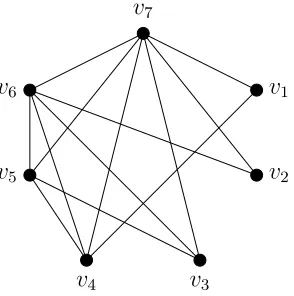
Let Hn denote an n-vertex graph with vertex set V(Hn) ={v1, v2, . . . , vn} and edge
set E(Hn) = {vivj : i+j > nand i 6= j}. This graph, which is known as the half
graph, has degree sequence n−1, n−2, . . . ,j2nk,jn2k, . . . ,2,1. See Figure 3.1 for an example half graph, H7. Since it is obvious that nodes with degrees 0 and n −1
cannot co-exist in the same graph, the half graph attains the maximum number of
distinct degrees.
v7
v1
v2
v3
v4
v5
v6
Figure 3.1 The half graph on seven vertices, H7.
For a graph G, denote by A(G) the number of non-zero elements in the JDV
of G. By routine counting, we see that A(Hn) = n(n−2)/4 + 1 if n is even and
A(Hn) = (n−1)2/4 if n is odd. Hence we have that
lim
n→∞
A(Hn)
n
2
=
1 2,
so about half the elements of the JDV of the half graph are non-zero. However, there
are constructions which achieve a higher number of non-zero elements in the JDV
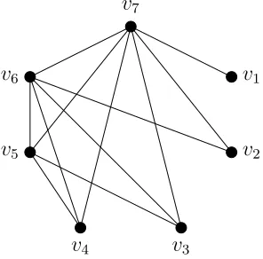
than the half graph. Consider the graph Hn with n ≥ 7 odd. If one connects the
degree 1 vertex to one of the vertices with degree (n−1)/2, the JDV elementj1,n−1 is
lost, but one gains new elements j2,(n+1)/2 and j(n+1)/2,(n+1)/2. We found even better
v7
v1
v2
v3
v4
v5
v6
Figure 3.2 A graph on seven vertices that achieves a higher number of non-zero elements in the JDV than the half graph, H7.
3.4 Two upper bounds
In this section, we provide two upper bounds that provide numerically very close
upper bounds, but use entirely different methods. Although we tried, we were unable
to combine these two proof techniques. We think that it is instructive to show both
of them. We note here that it was Aaron Dutle who first gave a non-trivial upper
bound (1−1/e+o(1))n2 = 0.63212...n2 for the number of non-zero entries in ann×n
JDM. His proof was somewhat similar to Subsection 3.4 but missed the symmetry
that is key to that subsection.
Continuous optimization
Let Pn = {(i, j) ∈ N2 : 1 ≤ i ≤ j ≤ n −1}. For any graph G, let A(G) :=
{(k1, k2)∈ Pn : jk1k2(G)>0}. The following identity is a simple consequence of the characterization of JDM matrices was written in this form in [43]:
Proposition 3.3. For any graph G,
X
(k1,k2)∈A(G)
k1+k2
k1k2
nk1k2(G) =n−n0(G), (3.2)
To see this, by Theorem 3.1 part (i) we have that
n−n0(G) =
n−1
X
i=1
ni(G) = n−1
X i=1 1 i i X k=1
jki(G) + n−1
X
k=i
jik(G)
!
= X
(k1,k2)∈A 1
k2
+ 1
k2
jk1k2(G) = X
(k1,k2)∈A
k1+k2
k1k2
jk1k2(G)
In the end, we are only interested in graphs without isolated nodes, since isolated
nodes do not contribute any edges. If a graph has more than one isolated node, then
we can connect the isolated nodes among each other. This can only increase the
support of the vector of bidgrees. Thus, there are optimal graphs with at most one
isolated node. On the other hand, connecting a single isolated node to a node of
degree d < n can reduce the support of the vector of bidegrees by at mostd. As we
have seen in Section 3.3, there are graphs where the support is of sizeO(n2). Hence, asymptotically, we can ignore single isolated nodes.
Corollary 3.4. For any graph G,
X
(k1,k2)∈A(G)
k1+k2
k1k2
≤ X
(k1,k2)∈A(G)
k1+k2
k1k2
nk1k2(G)≤n.
The original optimization problem can be formulated as follows:
• Maximize |A(G)| among all graphs G with n vertices.
Using the corollary, we relax this optimization problem and study the following
prob-lem, which we call thediscrete relaxation:
• Maximize the cardinality among all subsets A⊆Pn under the constraint
P
(k1,k2)∈A
k1+k2
k1k2 ≤n.
For anyn, the cardinality of a subset that solves the is an upper bound for the original
optimization problem.
The discrete relaxation can be solved on a computer as follows: First, compute
up as long as the sum does not exceedn. Finally, count the number of elements that
have been added. To compare the values for different n, let αn be the cardinality
of a solution A of the discrete relaxation divided by n2, the cardinality of Pn. The
values of αn are plotted in Figure 3.3. As a function of n, the optimum αn decreases
roughly (though not strictly) and reaches values below 0.56 for large n.
Figure 3.3 An upper bound for the ratio of maximum non-zero elements of the bi-degree vector to its length.
The limit for n → ∞ can be computed by approximating the discrete relaxation
by the following optimization problem, which we call the continuous relaxation:
• Maximize (n|A−01)|2 among all subsets A
0 ⊆[1, n]×[1, n] that satisfy
RR
A0 1
xdxdy ≤n.
10 20 30 40 50 60 70 80 90 100
0.55 0.6 0.65
n
ratio
αn α0n
Lemma 3.5 limn→∞αn
Figure 3.4 The solution of the discrete and continuous relaxation. The blue line plots the upper bound on αn from Lemma 3.5. The red line is the limit for large n
Letα0n be the maximum of the continuous relaxation.
Lemma 3.5. αn≤ n−n1α0n+
1
n.
Proof. To each (i, j)∈Pn associate the two squares Ai,j := [i, i+ 1)×[j, j+ 1) and
Aj,i := [j, j+1)×[i, i+1). ForA⊆PnletA00 =S(i,j)∈AAi,j andA0 =A00∪S(i,j)∈AAj,i.
Then
X
(i,j)∈A i+j
i·j ≥
X
(i,j)∈A
ZZ
Ai,j
x+y
x·y dxdy=
Z Z
A00
x+y x·y dxdy
≥ 1 2
Z Z
A0
x+y
x·y dxdy=
ZZ
A0
1
xdxdy.
Here, the first inequality follows from the fact that the maximum of xxy+y = x1 + y1 over Ai,j is at (x, y) = (i, j). The second inequality follows by not double-counting
the set Ad := S(i,i)∈AAi,i corresponding to the diagonal elements of A. The last
equality follows since xx+·yy = x1 + y1 and since A0 is symmetric along the diagonal. Therefore, if A is feasible for the discrete relaxation, then A0 is feasible solution for
the continuous relaxation. Now,
|A|=|A00|= 1 2(|A
0|
+|Ad|)≤
|A0| 2 +
n−1 2 ,
and so
αn≤
(n−1)2
2n2 α
0
n+
n−1
2n2 .
Corollary 3.6. lim supn→∞αn ≤lim supn→∞α0n.
It is not difficult to see that, actually, limn→∞αn = limn→∞α0n. Figure 3.3 shows
that the upper bound from Lemma 3.5 is not very close and suggests that αn ≤α0n;
at least forn ≤100.
Next, we want to solve the continuous relaxation. The idea is the following: As
the set A0 it is advantageous to choose a sublevel set of the function xx+·yy. For c >0 let
Ac :=
(x, y)∈[1, n]2 : x+y
x·y ≤c
Let
yc(x) =
1
c− 1
x
= x
xc−1, x1(c) =
1
c− 1
n
= n
nc−1.
Lemma 3.7. Ac =
(x, y)∈ [1, n]2 : x
1(c)≤ x≤ n, yc(x)≤ y≤ n
. In particular,
Ac6=∅ if and only if nc≥2.
Proof. Ifx < x1(c) and 1≤y≤n, then 1x+1y > c−1n+n1 =c. If x1(c)≤x≤n and
1 ≤y < yc(x), then x1 +y1 > c− x1 +x1 = c. For the second statement observe that x1(c)≤n if and only if nc≥2. Similarly, yc(x)≤n if and only if x≥x1(c).
Lemma 3.8. Assume thatc is such thatx1(c)≥1. Then yc(x)≥1for all x∈[1, n].
Proof. yc(x) decreases monotonically with x. Therefore, yc(x) ≥ yc(n) = x1(c) for
allx∈[1, n].
Lemma 3.9. Let n ≥3. The set Ac is feasible for the continuous relaxation if and
only if
(nc−2) log(nc−1)≤nc (3.3)
Proof. Assume that cis such that x1(c)≥1. Then
ZZ
Ac
1
xdxdy=
Z n
x1(c) dx
Z n
yc(x)
dy1
x =
Z n
x1(c)
dxn−yc(x) x
= Z n
x1(c) dx
n
x −
1
xc−1
=nlog n
x1(c)
− 1
clog
nc−1
cx1(c)−1
.
Now,
cx1(c)−1 =
cn−nc+ 1
nc−1 =
1
nc−1,
and so
ZZ
Ac
1
xdxdy=nlog(nc−1)−
1
clog(nc−1)
2 = (n− 2
c) log(nc−1).
Hence, Ac is feasible if and only if
Now suppose that n > e. If csatisfies (3.3), then
x1(c)≥
n
exp(nc/(nc−2)) >
n e >1.
Thus, the above calculation is valid and shows thatAcis feasible. On the other hand,
if n > e and if c violates (3.3), then Ac is not feasible.
To find the solution of the continuous relaxation, we need to find the value of c
that solves (3.3) with equality. Consider the equation
log(β−1) = β
β−2.
Both the left and the right hand side change sign at β = 2. For β > 2, both sides
are positive, and for β < 2 they are negative. By Lemma 3.7, we are looking for a
solution larger than 2. For β > 2, the right hand side is decreasing, while the left
hand side is increasing. It follows that there is a unique solutionβ0 >2. Numerically,
β0 ≈5.68050. Thus, Ac is feasible if and only if c≤ β0/n, and in order to maximize
|Ac|, we have to choose c=β0/n.
Lemma 3.10. x1(β0/n)>1 for n large enough.
Proof. x1(β0/n)−1 = n−β0β−0+11 >0 forn large enough.
It remains to compute the maximum value of the continuous relaxation. Ifx1(c)≥
1, then
|Ac|=
Z Z
A
dxdy= Z n
x1(c) dx
Z n
yc(x)
dy= Z n
x1(c)
dx(n−yc(x)).
Now,
yc(x) = 1
c x x− 1
c
! = 1
c 1 +
1/c x− 1
c
! = 1
c
1 + 1
cx−1
,
and so
|Ac|=
Z n
x1(c)
dx(n−1
c −
1/c
cx−1) = (n− 1
c)(n−x1(c))−
1
c2 log
cn−1
cx1(c)−1
=n2nc−1 nc
nc−2
nc−1 −
2
Therefore,
α0n= |Aβ0/n| (n−1)2 =
n2
(n−1)2
"
β0−2
β0
− 2
β2 0
β0
β0−2
#
= n
2
(n−1)2
(β0−2)2−2
β0(β0−2)
.
Numerically, α0n≈n2/(n−1)20.55225694.
Second Bound
Let G = (V, E) be an n-vertex graph and let A(G) be defined as in Section 3.4.
Let ni denote the number of vertices with degree i, with some m total number of
distinct vertex degrees. We callia single if ni = 1 and multiple if ni ≥2, noting that
someiare neither single nor multiple, they just don’t occur as degrees. As before, for
1≤i≤k ≤n−1, letjikbe the number of edges between theith andkth degree classes
andχik = 1 ifjik >0, and 0 otherwise. It is easy to see that|A(G)|=Pni=1−1
Pn−1
k=i χik.
Now we set setDi =Pi
k=1χki+
Pn−1
k=i+1χik andB(G) =
Pn−1
i=1 Di. Note that fork6=i,
Di counts χki =χik twice butχii is counted only once, so we get |A(G)| ≤ B(G)+2n−1 and therefore
|A(G)| n
2
≤
B(G) +n−1
2 ·
2
n(n−1) = (1 +o(1))
B(G)
n2 .
Our goal for this section is to prove the following theorem but first we proceed with
the proofs of several necessary lemmas.
Theorem 3.11. For any graph G,
|A(G)| n
2
≤(1 +o(1)) 13 24.
Lemma 3.12.
n−1
X
i=1
Di ≤
X
i:isingle
min(m, i) +√m
s X
i:imultiple
min(m, i) s
X
i:imultiple
ni.
Proof. Observe that Di ≤ m and Di ≤ ini, and hence Di ≤ min(m, ini). By case
of two elements is less than their average we get
Di ≤min(m,min(m, i)·ni)≤
q
m·min(m, i)·ni. (3.4)
Note that ifi is single we have
Di ≤min(m, i). (3.5)
Employing (3.4) and (3.5) we get that
n−1
X
i=1
Di ≤
X
i:isingle
Di+
X
i:imultiple
Di
≤ X
i:isingle
min(m, i) +√m X i:imultiple
q
min(m, i)·ni
≤ X
i:isingle
min(m, i) +√m
s X
i:imultiple
min(m, i) s
X
i:imultiple
ni, (3.6)
where the last inequality follows from Cauchy-Schwarz.
We wish to upper bound the term from (3.6) over all graphs G. From our lower
bound construction we know that |A(G)| ≥ (1−o(1))12n2. So we may assume that
m > n/√2, else we’d have |A(G)| ≤ m2 ≤n2/2 and our estimation of |A(G)| would
be complete.
Lemma 3.13. X
i:ni>0
min(m, i)≤m(n−m−1) + n(2m−n+ 1)
2 .
Proof. We wish to upper bound P
i:ni>0min(m, i) over all graphs. So assume the m
highest possible degrees occur in our graph:
n−1, n−2, . . . , n−m+ 1, n−m.
Now our assumption m > n/√2 gives that m > n−m+ 1, so the value of m has to
appear in the list of degrees above. There are n−1−m terms strictly larger thanm
Pm
i=n−mi, and hence
X
i:ni>0
min(m, i)≤m(n−m−1) +
m
X
i=n−m i
=m(n−m−1) + n(2m−n+ 1)
2 . (3.7)
Now if the m highest degrees do not occur in our graph, then some degree less than
n−m+1 must occur which clearly gives something smaller than the term in (3.7).
Now letsbe the number of degreesithat are singles. Observe we must haves ≤m
and s+ 2(m−s)≤n, implying that s≤m ≤ n+s
2 . Now usings+
P
i:i multipleni =n
and substituting
y= X
i:isingle
min(m, i)
z =
s X
i:imultiple
min(m, i),
we can write the term in (3.6) as
g(y, z, s, m) = y+√m·z√n−s.
We wish to maximize G subject to the constraints
1. All variables are non-negative and s≤n,
2. s≤m≤ n+s
2 , and
3. y+z2 ≤m(n−m−1) + n(2m−n+1) 2 ,
where constraint 3 follows from Lemma 3.13.
Y =P
i:isinglemin(m, i)/n, and Z =
q P
i:imultiplemin(m, i)/n and turn to the
follow-ing numeric optimization problem: maximize
f(Y, Z, S, M) =Y +√M ·Z√1−S
subject to the constraints
(a) All variables are non-negative andS ≤1,
(b) S ≤M ≤ 1+S
2 , and
(c) Y +Z2 ≤M(1−M) + 2M−1 2 .
By routine arguments, it follows that g(y, z, s, m)≤(1 +o(1))f(Y, Z, S, M)n2.
Lemma 3.14. If constraints (a), (b), and (c) hold, then
f(Y, Z, S, M)≤ 13 24.
Proof. For fixed values of S, M and Z, the function f is monotone in Y. Therefore,
we have to choose Y as large as possible, which, according to the last constraint,
implies that Y =−M2+ 2M − 1 2 −Z
2. Also the right hand side of constraint (c) is
non-negative if and only if 1−√2/2≤M ≤1 +√2/2, so 1−√2/2≤M ≤1.
Now for fixed values of Z and M the target function f decreases with S. Hence
we need to chooseSas small as possible. The constraints imply S ≥max{0,2M−1}
so we consider the following two cases.
If M ≤1/2, then S= 0. In this case, we need to optimize
f(Z, M) =−M2+ 2M − 1 2 −Z
2+√M·Z
subject to
1. 1−√2/2≤M ≤1/2,
The target functionf is quadratic inZ with maximum at Z0(M) =
√
M /2. Observe
that
f(Z0(M), M) = −M2+
9 4M −
1 2.
This function is quadratic in M, with maximum at M = 98 > 12. Therefore, it is maximized by the largest feasible M = 1/2. In total,
f(Z, M)≤f(Z0(M), M)≤f(Z0(1/2),1/2) =
3 8
for all feasible values of (Z, M). Finally, observe that (Z0(1/2),1/2) is feasible, since
Z0(1/2)2 =
1 8 <
1 4 =−
1 4 + 1−
1 2.
For the second case, suppose now that M ≥1/2. Then S = 2M−1, and we need
to optimize
f(Z, M) =−M2+ 2M− 1 2 −Z
2+√M·Z ·q2(1−M)
subject to
1. 1/2≤M ≤1,
2. Z2 ≤ −M2+ 2M − 1 2.
Nowf is quadratic inZ, with maximum atZ0(M) =
q
M(1−M)/2. To see that
(Z0(M), M) is feasible, we have to check that
0≤ −M2+ 2M − 1
2−Z0(M)
2 =−1
2M
2+3
2M − 1 2.
The right hand side is a quadratic polynomial with zeros at (3−√5)/2<1/2 and (3+ √
5)/2>1, which proves that (M, Z0(M)) satisfies all constraints.
Therefore, we need to maximize the quadratic function
f(M) = −M2+ 2M −1 2 +
1
2M(1−M) = − 3 2M
2+5
with 1/2≤M ≤1. The maximum is at M = 5/6, where the value is
f(5/6) =−75 72 +
25 12−
1 2 =
13
24 = 0.5416.
Proof (of Theorem 3.11). By Lemma 3.12 and Lemma 3.14,
B(G) =
n−1
X
i=1
Di
≤ X
i:isingle
min(m, i) +√m
s X
i:imultiple
min(m, i) s
X
i:imultiple
ni
=g(y, z, s, m)
≤(1 +o(1))f(Y, Z, S, M)n2
≤(1 +o(1))13 24n
2,
implying that
|A(G)| n
2
= (1 +o(1))
B(G)
n2 ≤(1 +o(1))
Chapter 4
Maximal matchings in polyspiro and benzenoid
chains
4.1 Introduction
Recall a matching in a graph is a collection of its edges such that no two edges in
this collection have a vertex in common. Matchings in graphs serve as successful
models of many phenomena in engineering, natural and social sciences. A strong
initial impetus to their study came from the chemistry of benzenoid compounds after
it was observed that the stability of benzenoid compounds is related to the existence
and the number of perfect matchings in the corresponding graphs. That observation
gave rise to a number of enumerative results that were accumulated over the course
of several decades; we refer the reader to monograph [11] for a survey. Further
motivation came from the statistical mechanics via the Kasteleyn’s solution of the
dimer problem [30, 31] and its applications to evaluations of partition functions for
a given value of temperature. In both cases, the matchings under consideration are
perfect, i.e., their edges are collectively incident to all vertices of G. It is clear that
perfect matchings are as large as possible and that no other matching in G can be
“larger” than a perfect one. It turns out that in all other applications we are also
interested mostly in large matchings.
Basically, there are two ways to quantify the largeness of a matching. One way, by
using the number of edges, gives rise to the idea of maximum matchings. Maximum